EVALUATION OF A MICROPILE LATERALLY LOADED USING SEMIEMPIRICAL, ANALYTICAL AND COMPUTATIONAL MODELS FOR GEOTECHNICAL ENGINEERING PRACTICE
CASE OF STUDY: SABANETA
LUIS VILLEGAS NEGRETTE
Dissertation submitted as partial fulfillment of the requirements for the degree of Master in Engineering
SUPERVISOR: JORGE ALONSO PRIETO SALAZAR
MEDELLÍN
EAFIT UNIVERSITY
SCHOOL OF ENGINEERING
Acceptance note
_______________________
_______________________
Chairman
_______________________
Examinator
_______________________
Examinator
_______________________
Medellín
ACKNOWLEDGMENTS
First, I would like to express my gratitude and admiration to my bosses Pedro Salvá and Bernardo Vieco, thanks for allowing me to use the information consigned on this document for the development of this research. Their valuable advice and accurate guidelines have helped me to become the professional I am.
I want to thank my advisor Jorge Alonso Prieto for his mentoring and supervision. Without his comments, this could not be possible.
I deeply want to recognize the labor of the engineers Laura Sierra and Camilo Pérez, thanks to their commitment with this project, without that, this research could not be conducted.
Thanks to MIDAS Information Technology Co., Ltd. for allowing me to use a full license of its software MIDAS GTS NX during the development of this research, without its unconditional help and the support of the MIDAS LA team this could not have been conceivable. I want to highlight the huge collaboration from Katerine Hincapie and Angel F. Martínez, thank you for your patience and great attitude.
I would also like to thank my friends and colleagues Alejandro Velásquez, Carellys Vergara and Jaime A. Mercado for their comments and suggestion about the structure of this document and their unconditional support during this process.
ABSTRACT
The Aburrá Valley’s demographic increase has risen house offering. To tackle this local issue, recently the use of micropiles have spread widely, even though this system has proven to be a reliable alternative foundation to support vertical loads, its capacity to support lateral loads has always been a concern. Considering this, this research focuses in the evaluation of the behavior of a type D micropile’s laterally loaded.
Two lateral load tests results are consigned and one of them is compared with results obtained from conventional methods used in practical engineering for lateral displacements estimation: semiempirical formulations, P-Y curves and three-dimensional finite element models.
The geotechnical parameters selection implications for the micropiles type D lateral displacement evaluation using semiempirical methods and P-Y curves are analyzed and briefly discussed. To recreate the triaxial tests stress-strain curves, some of the most practical constitutive soil models currently applied are revised. To evaluate the implications of the micropile injection process in the micropile lateral displacement estimation, a three-dimensional finite element model is used. Some alternative proposals for evaluation of the elastic behavior of a micropile laterally loaded are presented. Finally, conclusions are included, and some research topics are suggested.
KEYWORDS:
Micropile. Lateral load.
Lateral deformation. Semiempirical method. P-Y curves.
RESUMEN
El incremento poblacional en el Valle de Aburrá ha llevado al aumento de la demanda de la vivienda. Para atender esto y los problemas locales, el uso de micropilotes como sistema de cimentación se ha extendido en los últimos años, y a pesar de que ha demostrado ser un sistema confiable para atender cargas verticales, su capacidad para atender solicitaciones horizontales siempre ha quedado en duda. Por eso, este trabajo se enfoca en la evaluación del comportamiento de un micropilote tipo D sometido a cargas laterales.
Se presentan los resultados de dos pruebas de carga lateral y uno de ellos se compara con los métodos convencionales usados en la ingeniería práctica para la estimación de desplazamientos laterales: formulaciones semiempíricas, curvas P-Y y modelos de elementos finitos en tres dimensiones.
Las implicaciones de la elección de los parámetros geotécnicos para la evaluación del comportamiento lateral de micropilotes tipo D usando métodos semiempíricos y curvas P-Y son analizadas y levemente discutidas. Para recrear las curvas de Esfuerzo-Deformación de los ensayos triaxiales, se revisaron algunos de los modelos constitutivos más prácticos aplicados en la actualidad. Uno modelo tridimensional de elementos finitos es usado para evaluar las implicaciones del proceso de inyección de los micropiles en la estimación del desplazamiento lateral. Se presentan algunas propuestas alternativas para la evaluación del comportamiento elástico de un micropilote lateralmente cargado. Finalmente, se dan las conclusiones y recomendaciones para futuras investigaciones.
PALABRAS CLAVE: Micropilote. Carga lateral. Deformación lateral. Método semiempírico. Curvas P-Y.
TABLE OF CONTENTS
ACKNOWLEDGMENTS ... 4
ABSTRACT ... VI
RESUMEN ... VII
TABLE OF CONTENTS ... VIII
LIST OF FIGURES ...XI
LIST OF TABLES ... XIV
LIST OF ANNEXES ... XV
LIST OF SYMBOLS ... XVI
1
INTRODUCTION ... 1
1.1 OBJECTIVES... 2
1.2 SCOPE OF RESEARCH ... 2
2
BACKGROUND ... 3
2.1 MICROPILES ... 3
2.2 PILES LATERALLY LOADED ... 7
2.2.1 ULTIMATE LATERAL RESISTANCE ... 7
2.2.2 THEORY OF ELASTICITY ... 8
2.2.3 ELASTIC BEAM FOUNDATION ... 8
2.2.5 NAVFAC METHOD ... 12
2.2.6 NONDIMENSIONAL CHARTS ... 14
2.2.7 P-Y CURVES ... 15
2.2.8 CHARACTERISTIC LOAD METHOD ... 16
2.2.9 COMPUTATIONAL MODELS ... 16
2.3 MICROPILES LATERALLY LOADED ... 19
3
CASE STUDY ... 22
3.1 DESCRIPTION ... 22
3.2 GEOLOGICAL CHARACTERISTICS ... 23
3.2.1 MIGMATITAS DE PUENTE PELÁEZ (TRMPP) ... 23
3.2.2 DEPÓSITOS DE FLUJO DE LODOS Y/O ESCOMBROS (NQFII) ... 24
3.3 GEOTECHNICAL CHARACTERISTICS ... 24
3.3.1 SURVEY RESULTS ... 25
3.4 MICROPILES LOAD TESTS ... 32
3.4.1 VERTICAL LOAD TEST ... 35
3.4.2 LATERAL LOAD TEST ... 36
4
ANALYSES... 38
4.1 CURRENT PRACTICAL USED MODELS ... 38
4.2 MODELING ... 38
4.2.1 BEAM ON ELASTIC FOUNDATION USING SEMIEMPIRICAL FORMULATIONS ... 39
4.2.2 P-Y CURVES ... 44
4.2.3 COMPUTATIONAL MODEL ... 48
5
ADDITIONAL APPROACH ... 58
6.1 CONCLUSIONS ... 63
6.2 RECOMMENDATIONS ... 64
7
REFERENCES ... 66
LIST OF FIGURES
Fig. 1. Micropile classification system, a) Application classification Case 1, b) Application
classification Case 2 and c) Types of grouting. After (FHWA 2005). ...3
Fig. 2. Scheme of a hollow bar micropile. Adapted from (Abd El-aziz 2012). ...5
Fig. 3. Rotation required to mobilize active and passive earth resistance. After (Budhu 2015). ...7
Fig. 4. Coefficient of variation of subgrade reaction. After (NAVFAC 1986). ... 13
Fig. 5. Coefficients for long piles in cohesive soils. Adapted from (Das 2002). ... 15
Fig. 6. Project location. After Google Earth 2016. ... 22
Fig. 7. Regional geology. After (A.M.V.A 2007). ... 23
Fig. 8. Geotechnical survey location on the original terrain conditions. ... 24
Fig. 9. Location of field tests and micropiles vertically and horizontally tested. ... 26
Fig. 10. Summary of basic characterization laboratory tests. ... 27
Fig. 11. Summary of field tests and mechanical soil resistance based on some laboratory tests. ... 28
Fig. 12. Summary of soil parameters. ... 29
Fig. 13. NQfll's boulder. ... 30
Fig. 14. Res. V and Res. V (2) materials. ... 31
Fig. 15. Site conditions and micropile's reinforcement. ... 33
Fig. 16. Exhumed micropiles. ... 34
Fig. 17. Vertical load test - M-PC-V. ... 35
Fig. 19. SAP 2000 model. a) Micropile cross section, and b) 3D model. ... 41
Fig. 20. Comparison between lateral load test result against lateral response of a beam on elastic
foundation using semiempirical methodologies for: a) the lowest soil’s parameters, b) average
soil’s parameters, and c) the highest soil’s parameters. ... 43
Fig. 21. ALLPILE Model. a) micropile characteristics, b) the lowest soil’s parameters, c) average soil’s parameters, and d) the highest soil’s parameters. ... 44
Fig. 22. P-Y curves for: a) the lowest soil’s parameters, b) average soil’s parameters, and c) the highest soil’s parameters. ... 45
Fig. 23. Comparison between lateral load test result against lateral response of a beam on elastic foundation using P-Y curves method for: a) the lowest soil’s parameters, b) average soil’s
parameters, and c) the highest soil’s parameters. ... 47
Fig. 24. NQfll constitutive model evaluation. a) Mohr Coulomb model, b) Duncan-Chang model and c) Hardening Soil model. ... 49
Fig. 25. 3D model. a) soil layer and b) micropile element. ... 51
Fig. 26. Micropile characteristics. a) equivalent material properties and b) cross section. ... 51
Fig. 27. Lateral displacement evaluation at: a) micropile's head and b) along micropile's depth. .. 53
Fig. 28. Lateral displacement evaluation with NQfll’s reference modulus and OCR scaled. a)
micropile's head and b) along micropile's depth. ... 55
Fig. 29. Lateral displacement evaluation with NQfll Mohr Coulomb model using soil’s modulus
after injection. a) micropile's head and b) along micropile's depth. ... 56
Fig. 30. Soil shear stress conditions during a lateral load test. ... 59
LIST OF TABLES
Table 1. A values. After (Terzaghi 1955). ...9
Table 2. Values of 𝑘𝑠1 in kPa for square plates 30 cm x 30 cm and for long strips, 30 cm wide, resting on pre-compressed clay. Adapted from (Terzaghi 1955). ... 10
Table 3. 𝑘ℎ semiempircal formulations. ... 10
Table 4. Numerical values of m coefficient. After (Broms 1964a). ... 11
Table 5. Estimated values for 𝑘ℎ. Adapted from (Davisson 1970). ... 11
Table 6. 𝑛ℎ and 𝑘ℎ values. Adapted from (Robinson 1979). ... 12
Table 7. Coefficients for long piles in granular soils. Adapted from (Das 2002). ... 14
Table 8. Overview of model parameters and selection methods. Adapted from (Brinkgreve 2005). ... 18
Table 9. Basic Index and soil’s resistance parameters. ... 31
Table 10. NQfll layer moduli of subgrade reaction - semiempirical formulations - Lowest case. .... 39
Table 11. NQfll layer moduli of subgrade reaction - semiempirical formulations - Intermediate case. ... 39
Table 12. NQfll layer moduli of subgrade reaction - semiempirical formulations - Highest case. ... 40
Table 13. Constitutive soil parameters for each soil layer modeled with HS. ... 50
Table 14. Constitutive soil parameters for each soil layer modeled with MC. ... 50
Table 15. Evaluation of equations (2) to (4). ... 54
Table 17. Evaluation of coefficients of reduction due to slope proximity using (Mezazigh 1995). .. 60
Table 18. Moduli of subgrade reaction using proposed formulation and (Mezazigh 1995) methodology. ... 61
LIST OF ANNEXES
Annex 1- Res. V layer moduli of subgrade reaction - semiempirical formulations – Lowest case ... 72Annex 2. Res. V layer moduli of subgrade reaction - semiempirical formulations -Highest case. ... 72
Annex 3. Res. V (2) layer moduli of subgrade reaction - semiempirical formulations - Lowest case. ... 73
Annex 4. Res. V (2) layer moduli of subgrade reaction - semiempirical formulations - Highest case. ... 73
Annex 5. Res. IV layer moduli of subgrade reaction - semiempirical formulations - Lowest case. .. 73
Annex 6. Res. IV layer moduli of subgrade reaction - semiempirical formulations - Highest case. . 74
Annex 7. Lateral evaluation using P-Y curves - lowest case... 77
Annex 8. Lateral evaluation using P-Y curves - average case. ... 81
Annex 9. Lateral evaluation using P-Y curves – highest case. ... 85
Annex 10. Res. V. HS Model calibration. ... 86
LIST OF SYMBOLS
𝑇𝐿 Ultimate traction or compression micropile capacity
𝑞𝑠 Ultimate grout to ground bond strength
Ds Average bond diameter
Ls Bond length
𝐿0 Depth of influence
𝐸𝑝 Micropile’s elasticity modulus
𝐼𝑝 Micropile’s inertia
𝐸𝑠 Soil’s elasticity modulus
𝑃 Reaction intensity
𝑘 Supporting medium stiffness
𝑦 Beam’s deflection
𝑘ℎ Coefficients of horizontal subgrade reaction
𝑧 Depth of analysis below ground surface
𝑑 Pile’s width
𝛾 Effective unit weight
𝑘̅𝑠1 Basic coefficient of vertical subgrade reaction (for square area with width B = 30 cm)
𝑞𝑢 Unconfined compressive strength
φ’ Effective friction angle
𝜈 Poisson’s ratio
𝑒 Void ratio
𝑣𝑠 Shear wave velocities
𝐿 Pile length
𝑚 Coefficient
𝜎′ Vertical effective stress
𝑦𝑢 Ultimate displacement
𝑦𝑧 Lateral displacement
𝜃𝑧 Rotation
𝑁𝑞, 𝑁𝛾 Bearing capacity factors
N Number of blows per foot (30 cm)
y/d Normalized deflection
A, 𝑓, 𝐴𝑥, 𝐵𝑥, 𝐴𝜃, 𝐵𝜃, 𝐴𝑚, 𝐵𝑚, 𝐴𝑣, 𝐵𝑣, 𝐴𝑝′, 𝐵𝑝, 𝐴′𝑦, 𝐵′𝑦, 𝐴′𝑚, 𝐵′𝑚 Coefficients
𝑀 Moment applied at pile head
𝑀𝑧 Internal bending moment
𝑉𝑧 Internal shear force
Pc Characteristic load
𝑇 Characteristic length of the soil-pile system
τ Shear stress
𝐺 Shear modulus
𝛾 Shear strain
𝐹 Internal shear force
𝐴 Transversal area where shear force is acting
𝜌 Soil density
g Gravity
t Distance between micropile and slope crest
tlim Limit distance
r Reduction coefficient
1
INTRODUCTION
Over the last decades the Aburrá Valley’s population has grown significantly as it is presented by (Departamento Administrativo Nacional de Estadística 2017a), as a consequence, construction firms have been forced to intensify the housing offers and to improve their building practices in order to be more competitive and increase their income in a shorter period of time as it is inferred from the results of the (Departamento Administrativo Nacional de Estadística 2017b) buildings census.
To optimize the constructible areas, buildings of the Aburrá Valley are getting higher every day, what has resulted on a significant increase in service loads coming from the superstructure to the subsoil. For this reason, the need of a better understanding of subsoil conditions and the improvement of construction methods has become a constant.
Over the last 5 years, these construction firms have decided to buy micropile drilling rigs to reduce the direct cost of foundation systems, to avoid outsourcing and to have less time-consuming way to build foundations.
Even when the acquisition of micropile’s construction equipment has been a profitable investment for construction firms, the Geotechnical design possibilities have been reduced almost exclusively to micropiles solutions and the wordiness about the reliability of this foundation system has become a constant.
Traditionally, micropiles are designed using some methodologies like (Lizzi 1982) and (Bustamante 1985), or design guidelines as (FHWA 2005), (Ministère de l’Équipement des Transports 1993) and (Dirección General de Carreteras 2005); nevertheless, these methodologies or guidelines are focused on the design of this element for vertical loads, and its lateral load resistance is lightly discussed or just neglected.
During a seismic event, deep foundations need to support lateral loads due to the initial lateral movements of the soil mass and the consequential interaction between foundation elements and the kinematic forces coming from the superstructure. This has been discussed by several authors like (Zeevaert 1983) and (Thilakasiri et al. 2009).
For the structural design of laterally loaded foundation elements, commonly, structural designers replace the soil by elastic equivalent springs. For certain conditions, this simplification can be considered correct (Day and Mucillo 2014), nevertheless; the reliability of the geotechnical methods to estimate these springs is the real concern, because there are a lot of methodologies to estimate them, but rarely the lateral expected behavior is confronted with the real one measured.
Currently, there are several methodologies developed to evaluate the lateral resistance and displacement of piles built on a specific type of soil and for specific pile conditions, however; these were not directly established for micropile elements; for which the construction method, small diameter and high reinforcement area are variables that are not considered on the actual lateral pile resistance formulation.
1.1
OBJECTIVES
To evaluate some current geotechnical methodologies used for lateral evaluation of deep foundations, analyzing their applicability to IRS micropiles built on the Aburrá Valley based on results of an IRS micropile laterally loaded.
- To perform a micropile lateral load test.
- To evaluate semiempirical moduli of subgrade reaction and their reliability. - To calibrate a practical soil constitutive model to represent soils behavior. - To simulate micropile lateral load test measurements.
1.2
SCOPE OF RESEARCH
2
BACKGROUND
2.1
MICROPILES
Micropiles are a type of deep foundation solution conceived by (Lizzi 1950) as a technique for underpinning historical buildings affected by World War II.
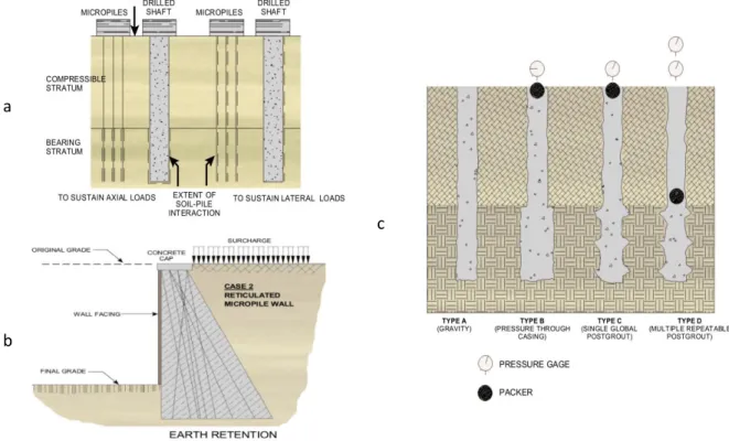
The use of micropiles has extended from its original function. Nowadays, they are used to improve soils resistance and as foundation solution. Micropiles can be classified according to their use or construction grouting technique (FHWA 2005). Fig. 1 shows the (FHWA 2005) classification system.
a
c
b
Fig. 1. Micropile classification system, a) Application classification Case 1, b) Application classification Case 2 and c) Types of grouting. After (FHWA 2005).
The grouting (FHWA 2005) classification system is similar to DTU 13.2 used in France (L’École
Nationale des Ponts et Chaussées 2004). The association and description of each classification system is shown below.
• Type A or II: foundation elements grouted by a sand-cement mortar or cement grout; placed by gravity head and non-injected.
• Type B or I: micropile’s neat cement grout is placed into a pre-bored hole using injection pressure lower than in-situ lateral soil pressure to avoid hydrofracturing of surrounding soil. Typically, this injection pressure is lower than 1 MPa.
• Type C or III: is a two-stage procedure, the first stage, a micropile Type A is developed. In the second stage (15 to 25 minutes later), the grouting procedure is repeated applying a higher lateral injection pressure, which is close to the pressuremeter limit pressure and in all cases higher than 1 MPa. This kind of injection is worldwide known as IGU (Injection Globale et Unitaire).
• Type D or IV: as Type C, this methodology is a two-stage procedure. In the first one, a micropile Type B is constructed, and in the second one (after grouting has hardened), additional grout is injected using lateral pressures higher than pressuremeter limit pressure; commonly this pressure ranges between 2 to 8 MPa. This procedure can be performed several times as it is required and it is commonly known as IRS (Injection Répétitive et Sélective).
Fig. 2. Scheme of a hollow bar micropile. Adapted from (Abd El-aziz 2012).
Generally, a micropile is also characterized by its small diameter (less than 300 mm), slender ratios greater than 100 (L’École Nationale des Ponts et Chaussées 2004) and its mechanism of resistance.
Micropiles are usually designed to support vertical loads by considering only their lateral resistance capacity and neglecting their point capacity. The typical formulation used for the geotechnical design of these elements is shown on (1).
𝑇𝐿= qs π D𝑠 Ls (1)
where, 𝑇𝐿 is the ultimate traction or compression capacity, 𝑞𝑠 is the ultimate grout to ground
bond strength, Ds is the average bond diameter, and Lsis the bond length.
Some practical values and formulations i.e. (Bustamante 1985; Dirección General de Carreteras 2005; FHWA 2005) have been used to evaluate 𝑞𝑠. Nevertheless, this parameter is not just function
important too. Taking into a count all these variables, load testing probes are commonly required to verify design assumptions.
On the other hand, for (FHWA 2005) one of the greatest limitations of micropiles is their lateral capacity. Sometimes, the main concern is just the vertical load, however, this conception is a mistake, particularly during a seismic event, where kinematic forces will result in a considerable lateral force requirement for the foundation system. As it is pointed out by (Richards and Rothbauer 2004), lateral load case often governs the design of micropiles and not just the vertical case.
Currently, lateral capacity of micropiles is estimated using theories developed for pile foundations, which do not consider the effect of the small diameter, the reinforcement controlling function and the installation method.
Sometimes, micropiles work as a group because they are connected by a cap to guarantee their unity. When a lateral solicitation exists, it is common to use a passive earth pressure resistance acting on the lateral side of the cap to verify its stability. Nevertheless, the ratio of displacement needed to develop a passive earth pressure on the cap can be excessive when it is compared to the elastic lateral displacement capacity of a micropile. Thus, a plastic hinge will be produced at certain depth. Consequently, micropiles will not be able to support the service loads coming from the superstructure.
To evaluate the influence of the lateral load on the micropile element, some formulations have been proposed. Equations (2) to (4) are some of the most used.
Author Equation
(FHWA 2005) 𝐿0= 20Ds (2)
(Richards and Rothbauer 2004) 𝐿0= 2 to 5 m (3)
(L’École Nationale des Ponts et Chaussées 2004) 𝐿0= √ 4𝐸𝑝𝐼𝑝
𝐸𝑠
4
(4)
where, 𝐿0 is the depth of influence, 𝐸𝑝 is the micropile’s elasticity modulus, 𝐼𝑝 is the micropile’s
inertia, and 𝐸𝑠 is the soil modulus of elasticity
2.2
PILES LATERALLY LOADED
The evaluation of a pile laterally loaded can be performed based on its ultimate lateral resistance or by its allowable lateral displacement.
2.2.1
ULTIMATE LATERAL RESISTANCE
Some of the most common methodologies used to evaluate ultimate lateral resistance of soil were proposed by authors like (Brinch-Hansen 1961) and (Broms 1964a; b).
Brinch Hansen method assumes that the pile is rigid and no yield hinge can be developed, so the pile rotates as a rigid body at a certain point below the ground surface.
The above-mentioned assumptions consider that Rankine’s passive earth pressure will be developed in front of the pile, and at the same time, behind the pile the active earth pressure will take place.
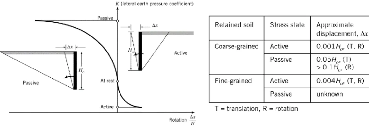
To develop passive earth pressure, lateral displacements are needed to be allowed, this displacement can be as large as a value close to 10% of a cantilever (pile’s length), as it is shown on Fig. 3, where is presented the displacement needed to reach an earth pressure of a specific type of
soil as a function of cantilever’s height.
Brinch Hansen methodology can be used to estimate the ultimate lateral resistance of a pile-soil system, however, this method is not able to evaluate lateral displacements as is noted by (Ruigrok 2010).
Alternatively, Broms’ formulation can be used to compute lateral deflections, ultimate lateral resistance and maximum bending moments for free head or restricted driven piles into saturated cohesive and cohesionless soils.
Broms proposed his formulation based on elastic theory to determine the behavior of pile element
and soil’s support reaction, he also considered that failure happens when pile’s section ultimate
stress or supporting soil ultimate stress is achieved.
To estimate the ultimate lateral resistance of soil, the author assumed that when a long pile is used a plastic hinge will take place at a certain depth, and that above it, the full passive resistance of soil will be developed.
Broms’ method was established based on available lateral load test results, which at his time were limited, this is the reason why he recommended using his methodology with caution.
2.2.2
THEORY OF ELASTICITY
This theory expresses the elastic stress-strain relationship of a material based on Hooke’s law as it is mentioned by (Timoshenko and Goodier 1951).
2.2.3
ELASTIC BEAM FOUNDATION
𝑃 = 𝑘 𝑦 (5) Where, 𝑃 is the reaction intensity, 𝑘 is the supporting medium stiffness, and 𝑦 is the beam’s
deflection.
Equation (5) involves that reacting medium is elastic; its constitutive material follows Hooke’s law and 𝑘 is a constant of proportionality that is just valid for the specific point of evaluation.
Using the elastic beam foundation formulation, a discretization of the element loaded, the flexural stiffness of a beam, equilibrium equations and differential procedures, is then possible to partially formulate equations to determine the internal forces of elements perpendicularly loaded. However, it is not possible to solve it directly and it will require the use of boundary conditions evaluations to find some integration constants. A detailed discussion of these formulations can be found on (Hetényi 1946).
2.2.4
SEMIEMPIRICAL FORMULATIONS
Several authors had formulated semiempirical coefficients of horizontal subgrade reaction (𝑘ℎ)
based on the elasticity theory and pile lateral load test literature reported or developed by them.
One of the first authors who proposed a semiempirical formulation was (Terzaghi 1955). He developed independent formulations for sands and clays.
For sands, he considered that 𝑘ℎ depends on the depth of analysis below ground surface (𝑧), pile’s
width measured at right angles to the direction of projected lateral displacement (𝑑), the effective unit weight (𝛾) and relative density of sand. As a result, the following formulation was proposed.
𝑘ℎ= 𝐴 𝛾 𝑧 1.35 𝑑
(6) where, A is a coefficient, see Table 1.
Table 1. A values. After (Terzaghi 1955).
Relative density of sand Loose Medium Dense
Range of values of A 100-300 300-1000 1000-2000
Another form to present (6) is substituting 1.35𝐴 𝛾 value by 𝑛ℎ, what results in (7).
𝑘ℎ= 𝑛ℎ 𝑧 𝑑
(7)
For piles embedded in stiff clays, the 𝑘ℎ value is supposed to be constant with depth and is just
function of pile’s width. According to (Terzaghi 1955) this value can be estimated using (8).
𝑘ℎ= 𝑘̅𝑠1 1.5 𝑑
(8) where, 𝑘̅𝑠1 is the basic value of coefficient of vertical subgrade reaction (for square area with
width B = 30 cm).
Suggested values proposed by (Terzaghi 1955), are shown on Table 2.
Table 2. Values of 𝑘̅𝑠1 in kPa for square plates 30 cm x 30 cm and for long strips, 30 cm wide, resting on pre-compressed
clay. Adapted from (Terzaghi 1955).
Consistency of clay Stiff Very stiff Hard
Values of 𝑞𝑢 (kPa) 95 – 191.5 191.5 - 383 > 383
Range for 𝑘̅𝑠1, square plates 50 - 100 100– 200 > 200
Proposed values, square plates 75 150 300
Various authors have used the same Terzaghi’s formulation and have derivated 𝑛ℎ and 𝑘ℎ values
for specific conditions. Some of the most common used on engineering practice are presented on the following table.
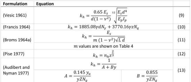
Table 3. 𝑘ℎ semiempircal formulations. Formulation Equation
(Vesic 1961) 𝑘ℎ=
0.65 𝐸𝑠 𝑑(1 − 𝜈2) √
𝐸𝑠𝑑4 𝐸𝑝𝐼𝑝
12
(9)
(Francis 1964) 𝑘ℎ= 1885.08𝛾𝑑𝑁𝛾+ 3770.16𝛾𝑧𝑁𝑞 (10)
(Broms 1964a) 𝑘ℎ=
𝐸𝑠
𝑚 (1 − 𝜈2)√𝐿 𝑑 (11)
𝑚 values are shown on Table 4
(Pise 1977) 𝑘
ℎ= 𝑛ℎ𝑧 2 3 (12) (Audibert and Nyman 1977) 𝑘ℎ= 1 𝐴 + 𝐵𝑦 (13) 𝐴 =0.145 𝑦𝑢
𝑦𝑍𝑁𝑞
𝐵 =0.855
(Kishida and
Nakai 1977) 𝑘ℎ=
1.3 𝐸𝑠 𝑑(1 − 𝜈2) √
𝐸𝑠𝑑4 𝐸𝑝𝐼𝑝
12
(14) (Robinson
1979) 𝑘ℎ= 67
𝑆𝑢
𝑑 (15)
(Bhushan et al. 1981)
log 𝑙𝑘ℎ= 0.82 + log 𝑁 − 0.62 log 𝑦
𝑑 (16)
𝑘ℎ= 271.447 (100.82+ log 𝑁−0.62 log 𝑦
𝑑) (17a)*
(Sogge 1981) 𝑘ℎ= 314.18 𝑡𝑜 4712.7
𝑧
𝑑 (18)
(Pyke and
Beikae 1984) 𝑘ℎ= 2
𝐸𝑠 𝑑 (19) (Habibagahi and Langer 1984) 𝑘ℎ= 𝜎′𝑁𝑞 𝑦 (20) 𝑁𝑞 = 𝐴 + √ 𝑧 𝑑
For 30°, A = 5,9,12 and 15 for y=2.54, 6.35, 12.7
and 25.4 mm
where, 𝐸𝑠 is the soil modulus of elasticity, 𝐸𝑝 is the pile elasticity modulus, 𝐼𝑝 is the pile inertia, 𝜈 is the Poisson’s ratio, 𝐿 is the pile length, 𝑚 is the coefficient, see Table 4, 𝜎′ is the vertical effective stress, 𝑦𝑢 is the ultimate displacement, 𝑁𝑞 and 𝑁𝛾 are the bearing capacity factors, N
is the SPT resistance over the embedded length of pile (blows/ft), y/d is the normalized deflection (%), and 𝑙𝑘ℎ is the coefficient of subgrade reaction (lb/in3).
*International System Adapted equation (kPa/m).
Table 4. Numerical values of m coefficient. After (Broms 1964a).
L/d 1.0 1.5 2 3 5 10 100
m 0.95 0.94 0.92 0.88 0.82 0.71 0.37
Even though several authors proposed some mathematical formulations for 𝑘ℎlike those shown on
Table 3, others preferred to use intervals.
(Davisson 1970) suggested some 𝑛ℎ and 𝑘ℎ values based on his personal experience and literature
reported values, see Table 5.
Table 5. Estimated values for 𝑘ℎ. Adapted from (Davisson 1970).
Soil type Value
Granular soils 𝑛ℎ ranges from 1.5 to 200 lb/in3; is relative proportional to relativity
density Normally loaded organic
silt
𝑛ℎ ranges from 0.4 to 3 lb/in3
Cohesive soils 𝑘ℎ is approximately 67 𝐶𝑢
Based on field test data of lateral load test on timber piles in cohesionless soil, (Robinson 1979) suggested that 𝑘ℎ is independent from pile’s width, and recommended the use of 𝑘ℎ and 𝑛ℎvalues
presented on Table 6.
Table 6. 𝑛ℎ and 𝑘ℎ values. Adapted from (Robinson 1979).
Soil Conditions Horizontal Subgrade Reaction
Soil description N Su, (kPa)
Horizontal movement
(mm) Type
Value Compute from Deflection (kPa)
Amorphous peat <1 26.42 𝑘ℎ 689.47
3ft sand 9.52 𝑘ℎ 3447.38
over amorphous
peat 𝑘ℎ 689.47
4ft gravelly clay 38.3 7.87 𝑘ℎ 5102.12
over clayey silt 1.5 19.1 𝑘ℎ 2551.06
5ft stiff clay 3 57.4 9.40 𝑘ℎ 3447.38
over silt and peat 1 19.1 𝑘ℎ 2068.43
Organic clay silt <1 14.4 15.24 𝑘ℎ 113.76
Layered silty sand 3 22.86 𝑛ℎ 206.84
and sandy silt
Layered sand and 5 6.35 𝑛ℎ 427.47
sandy silt
3.5ft sand 10 2.79 𝑛ℎ 1765.06
over clayey silt 4
Silty sand 5 6.09 𝑛ℎ 689.47
Slightly organic
silt 2 16.26 𝑛ℎ 103.42
3ft organic silt 1 17.27 𝑛ℎ 234.42
over sandy silt 3
It is important to notice that some theories have been originally developed for vertical subgrade modulus, nevertheless, they are often used to estimate lateral behavior. Some of the most common used are (M.A.Biot 1937), (Skempton 1951) and (Broms 1964a).
2.2.5
NAVFAC METHOD
soils and normally consolidated cohesive soil 𝑘ℎ is assumed to increase linearly with depth, this is
expressed by (21).
𝑘ℎ= 𝑓 ∗ 𝑧
𝑑 (21)
where, 𝑓 is the coefficient of variation of lateral subgrade reaction (ton/ft3), see Fig. 4.
Fig. 4. Coefficient of variation of subgrade reaction. After (NAVFAC 1986).
2.2.6
NONDIMENSIONAL CHARTS
This method derives from the differential equation for beam-column on a foundation given by (Hetényi 1946), the elasticity principles and some fundamental identities. Based on these principles the following equations can be defined for granular soils.
𝑦𝑧 = 𝐴𝑥 𝑃𝑇3 𝐸𝑝𝐼𝑝 + 𝐵𝑥 𝑀𝑇2 𝐸𝑝𝐼𝑝 (22) 𝜃𝑧= 𝐴𝜃 𝑃𝑇2 𝐸𝑝𝐼𝑝 + 𝐵𝜃 𝑀𝑇 𝐸𝑝𝐼𝑝 (23)
𝑀𝑧= 𝐴𝑚𝑃𝑇 + 𝐵𝑚𝑀 (24)
𝑉𝑧 = 𝐴𝑣𝑃 + 𝐵𝑣 𝑀 𝑇 (25) 𝑝′𝑧 = 𝐴𝑝′ 𝑄 𝑇+ 𝐵𝑝′ 𝑀
𝑇2 (26)
where, 𝐴𝑥, 𝐵𝑥, 𝐴𝜃, 𝐵𝜃, 𝐴𝑚, 𝐵𝑚, 𝐴𝑣, 𝐵𝑣, 𝐴𝑝′, 𝐵𝑝′ are coefficients (see the table), 𝑀 is the
moment applied at pile head (kN*m), and 𝑇 is the characteristic length of the soil-pile system. 𝑇 = √𝐸𝑝𝐼𝑝
𝑛ℎ
5
𝑍 =𝑧
𝑇
Table 7. Coefficients for long piles in granular soils. Adapted from (Das 2002).
Z 𝑨𝒙 𝑨𝜽 𝑨𝒎 𝑨𝒗 𝑨𝒑′ 𝑩𝒙 𝑩𝜽 𝑩𝒎 𝑩𝒗 𝑩𝒗
3.0 -0.075 -0.040 0.225 -0.349 0.226 -0.089 0.057 0.059 -0.213 0.268 4.0 -0.050 0.052 0.000 -0.106 0.201 -0.028 0.049 -0.042 0.017 0.112 5.0 -0.009 0.025 -0.033 0.015 0.046 0.000 -0.011 -0.026 0.029 -0.002 For cohesive soils
𝑦𝑧 = 𝐴′𝑥 𝑃𝑅3 𝐸𝑝𝐼𝑝
+ 𝐵′𝑥 𝑀𝑅2 𝐸𝑝𝐼𝑝
(27)
𝑀𝑧 = 𝐴′𝑚𝑃𝑅 + 𝐵′𝑚𝑀 (28)
where, 𝐴′𝑦, 𝐵′𝑦, 𝐴′𝑚, 𝐵′𝑚 are coefficients (see the following figure) 𝑅 = √𝐸𝑝𝐼𝑝
𝑘 4
𝑘, see equation (9)
Fig. 5. Coefficients for long piles in cohesive soils. Adapted from (Das 2002).
2.2.7
P-Y CURVES
This method is based on results of pile lateral load tests instrumented with strain gauges along its depth for different specific soil conditions and pile geometries.
Some of the first researchers that defined the p-y curves concept were (McClelland and Focht 1958); after them, numerous studies were done to evaluate the lateral behavior of several kind of piles under different subsoil conditions. Even though all that information was available, there was not a clear procedure to analyze the lateral behavior of piles laterally loaded under specific soil conditions,
that’s why, all that information was gathered and analyzed by several authors i.e. (Matlock 1970), (Welch and Reese 1972), (Reese et al. 1974), (Reese and Welch 1975), (Murchinson 1983), and others. They developed step by step methodologies to simulate P-Y curves for specific conditions. These detailed procedures are used by commercial software e.g. LPile, PileLAT 2014, PyPile, ALLPILE and others; detailed information can be found on (Reese et al. 2002) or in software’s technical manuals.
2.2.8
CHARACTERISTIC LOAD METHOD
As a practical approach, (Duncan et al. 1994) proposed the Characteristic Load Method which is a simplification of P-Y curves results, which is based on pile’s geometry, pile’s head restrictions, pile’s
material properties; and soil’s resistance.
Using dimensionless axes charts, lateral deflection and bending moments can be assessed as a function of characteristic load (Pc) and the characteristic moment (Mc).
Based on (Duncan et al. 1994) the charts are suitable to be used as a hand computation; however, this method is limited to piles and drilled shafts piles, and should not be used to estimate the lateral behavior of deep foundations in stiff clay subjected to cyclic loadings.
2.2.9
COMPUTATIONAL MODELS
Thanks to the advances on computational methods, many additional variants can be considered to evaluate their significance into an engineering problem. This particularity reveals the advantages of computational models to be used as a tool to evaluate what if scenarios.
The user of a computational tool must consider the mathematical restrictions and implications involved in the use of a software of Finite Elements or Finite Differences, or a Plain Strain Model, Axisymmetric Model or a 3D Model.
Even when the computational knowledge is required, if the final user concerning is about a geotechnical simulation, he also may understand the hypothesis, advantages, limitations and how the get the parameter of the constitutive soil model available.
According to (Brinkgreve 2005) the most commonly used geotechnical models for practical purposes
are Hooke’s law (LE), the Mohr-Coulomb model (MC), the Drucker-Prager model (DP), the Duncan-Chang model or Hyperbolic model (DC), the Cam-Clay model (CC), the Soft Soil (Creep) model (SS(c)) and the Hardening Soil model (HS).
Table 8. Overview of model parameters and selection methods. Adapted from (Brinkgreve 2005). Par ame te rs M o d e ls O e d o me te r C R S
CD CU UU DSS
To
rv
an
e
SPT CPT PM DM
T V an e te st C lassi fi cati o n Tab le s, r u le s
C’ MC, DP, DC, SS(C), HS
D D D C C
Φ’ MC, DC, SS(C), HS
D D D C C
M (friction)
DP, CC I I I I I
Su MC, DP, DC, HS D D C C D C C
Ψ MC, HS D C
E LE, MC, DP I I I I I I C C C C C
E50ref DC, HS I C D I D I I I C C
Eurref DC, HS (D) (D) (I) (D) I C
Eoedref HS D D I I I I C C C
λ (*) CC, SS(C) D I C I I C C
K (*) CC, SS(C) (D) I C I C
μ * SSC (D) D C
V LE, MC, DP, DC I D C
Vur CC, SS(C), HS (I) C
m (power)
DC, HS D I D D C C
Konc SS(C), HS (D) C C
Rf DC, HS C
where, D means directly, (D) means directly and recalculation is needed, I means indirectly, (I) means indirectly and recalculation is needed, and C means correlation.
The parameters for most of the constitutive soil models mentioned on the previous table can also be obtained from triaxial tests. These tests may be performed and instrumented in coherence with the characteristics that are going to be evaluated.
The model failure criterion is the Mohr-Coulomb, then, its strength parameters are needed (φ’ and
C’). As the model has a hyperbolic relationship, a failure ratio (Rf) must be defined.
For the primary loading, the confining stress dependent secant stiffness modulus for primary loading (E50) is needed. To relate it to different stress values, this modulus is a function of a stress referenced modulus (E50ref), normally referenced to a 100 kPa stress (pref). In addition to this, a power coefficient is used (m) to consider its stress dependency as a logarithmic function. The m value will depend of the level of stress used and the material.
The same function is applied for the unloading and reloading stress paths, but, the modulus that ought to be applied for this stress paths (Eurref) is the Young’s modulus; therefore, the unloading and reloading stress path is elastic. Due to it, the Hooke’s law must be satisfied, and the elastic strains computed using the Poisson’s ratio for the unloading and reloading (νur) strain estimation.
The plastic potential function adopted for the flow rule involves the use of the dilatancy angle (Ψ). On the other hand, the plastic strain originated from the yield cap is controlled by the tangent stiffness modulus for primary oedometer loading (Eoedref) and the coefficient of earth pressure at-rest for normally consolidated conditions (K0NC).
2.3
MICROPILES LATERALLY LOADED
After the results of eight lateral tests reported by (Plumelle and Raynaud 1996), the concern about the small lateral capacity of micropiles has become a constant. For that reason, the analysis of micropile laterally tested literature has increased.
Ten lateral load tests were conducted by (Long et al. 2004) to compare the behavior predicted using P-Y curves computed by LPILE software and the measures recorded on laterally loaded micropile field tests. As a result, he concluded that predicted and measured was in reasonably good agreement and that differences between measured and predicted was about ±10 percent.
results of those tests exposed that deflections can be overestimated by these methods, but they correspond to a conservative approach.
In both works, these authors agree with the importance of a good parameter identification of the upper 5 m and highlight the influence of the flexural stiffness in the behavior of the laterally loaded micropile.
In North Carolina, (Babalola 2011) installed sixteen micropiles which were prescribed on a depth of rock to perform nine single lateral load tests and a micropile group load test. He compared his results with the P-Y curves generated by FB-MultiPier software and analyzed the sensitivity of input parameters used.
Different types of vertical and lateral tests were performed by (Abd El-aziz 2012) on hollow bar micropiles built on a superficial thick layer of overconsolidated clayey silt to silty clay soil, overlying a compact sand deposit; within those tests, two monotonic lateral load tests were performed to compare them to predicted behavior by mean of P-Y curves computed by LPILE. Thus, the research concluded that some adjustments are needed on the parameters used to compute the P-Y curve to represent the measurements. These adjustments involved the use of parameter values not even reported on the original formulation of P-Y curves for the type of soil of the site of study.
As an extension of (Abd El-aziz 2012) works, (Osama F. 2013) resolved to conduct eight lateral tests on micropiles built on cohesive soils to compare his results with LPILE estimated behavior. He built two of the eight micropiles using 18 cm of diameter and the other six with 23 cm of diameter. As result of his research, P-Y curves fitted better for the highest diameter micropile.
(Kershaw and Luna 2014) analyzed the effect of vertical loads on the performance of lateral load tests of single micropiles installed at a clay and shale site. According to their results, the vertical load has a minimal effect on the lateral behavior of micropiles installed in stiff clay.
3
CASE STUDY
3.1
DESCRIPTION
The case study is in Sabaneta, Colombia; close to Sabaneta’s downtown as it is presented in Fig. 6
(see project’s pin). The project is a residential complex of 10 buildings with 28-stories, vertical service loads at foundation level between 6.7 and 15.6 MN and lateral seismic loads of 6 MN per support. Both loads were obtained using the NSR-10 guideline.
Fig. 6. Project location. After Google Earth 2016.
3.2
GEOLOGICAL CHARACTERISTICS
According to (Área Metropolitana del Valle de Aburrá 2007), the geological units that surround the project site are soils derived from rocks that belong to Grupo El Retiro in the Complejo Cajamarca, which is composed by Esquistos de Cajamarca (TReC) and Migmatitas de Puente Peláez (TTmPP).
At the same time, there are different types of soil deposits: alluvial (Qal or Qat) and mudflow with debris (NQFll), and in some places, are anthropic fills (Qll). This is illustrated on Fig. 7.
Fig. 7. Regional geology. After (A.M.V.A 2007).
3.2.1
MIGMATITAS DE PUENTE PELÁEZ (TRMPP)
3.2.2
DEPÓSITOS DE FLUJO DE LODOS Y/O ESCOMBROS (NQFII)
Corresponds to soils deposited with variable thickness (around two meters) which are mud-flows mud-supported with sub-angular boulders of gneiss, shales and quartz.
3.3
GEOTECHNICAL CHARACTERISTICS
To identify the geotechnical characteristics of the underlaying soil, a geotechnical survey program had been done for 5 of the 10 buildings projected. The survey involved 28 (22 in the original site conditions and 6 posteriors to excavations) Standard Penetration Tests (SPT), 6 Down Holes (DH) and 8 geophysical linear arrays of seismic analysis of surface wave (SASW) methods (1 of theses was performed after micropiles construction and beside them). These field tests were located as shown in Fig. 8.
Based on field test results, visual inspection of samples and some laboratory test results, it was possible to identify the geotechnical characteristics of each of the materials that constitute the soil profile.
Each sample obtained from SPT was visually described and some of them were chosen for laboratory tests. Disturbed samples were used to make a basic geotechnical characterization based on water contents, density, specific gravity, the Unified Soil Classification System (USCS), and gravimetric and volumetric relationships. On the other hand, undisturbed samples were selected to determine their undrained and drained soil resistance parameters using unconfined compression tests, consolidated drained direct shear tests and consolidated undrained compressional triaxial test with pore pressure record.
3.3.1
SURVEY RESULTS
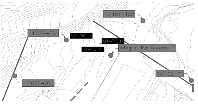
Micropiles vertically (M-PC-V) and horizontally tested (M1-PC-H and M2-PC-H) were located as it is shown in Fig. 9. It is also shown in this figure, the location of the closest field tests which are: SPT
Fig. 9. Location of field tests and micropiles vertically and horizontally tested.
Even though not all the triaxial tests were done on the field tests shown in the previous figure, they were made on the same material. These laboratory tests will be used in the following chapters, then a brief discussion will take place there.
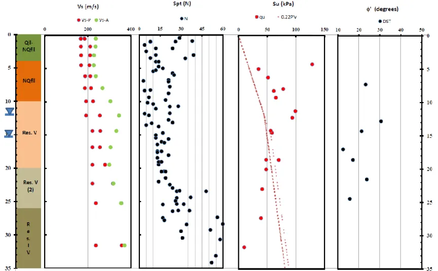
Fig. 10 summarizes the results of index laboratory tests including classification based on the USCS, content of fines, void ratio, dry and total densities and water content. Fig. 11 supplements the index laboratory tests with the soil resistance parameters obtained from laboratory tests, field exploration program results (shear wave velocities previous to micropiles construction - vs-P- and after micropiles construction - vs-A, and SPT blow counts) and the adopted soil profile.
The most superficial layer of the simplified geotechnical profile corresponds to man-made fills conformed during the construction of existing buildings that were located on project site. This layer, was entirely removed during construction of current project execution, therefore it will not be further discussed.
NQfll layer is a heterogeneous material with boulders as those shown on Fig. 13 and a soil matrix classified as silty sands and silty clays as is illustrated on Fig. 10.
Fig. 13. NQfll's boulder.
Under this layer, a residual soil profile is easily identified by its characteristic texture derived from
Fig. 14. Res. V and Res. V (2) materials.
In the following table, a summary of the index and the resistance Mohr coulomb’s soil parameters
for each layer is presented.
Table 9. Basic Index and soil’s resistance parameters.
Layer e W (%) γ (kN/m
3) Su (kPa) C’ (kPa) Φ’ (°) E s (kPa)
Min (m) Max (M) m M m M m M m M m M m M
NQfll 0.9 1.4 18 50 16 19 34 128 11 27 20 38 3 35
Res. V 1.0 1.6 42 58 16 18 48 99 4 53 20 29 4 52
Res. V (2) 0.7 1.3 32 54 17 19 39 41 30 34 23 31 12 55
3.4
MICROPILES LOAD TESTS
As it was mentioned previously, three load tests were performed at project site, those were performed following the guidelines of as per ASTM D 1143 and ASTM D 3966. The results of these tests are presented and briefly discussed on next paragraphs; but it is important to mention that:
• 4 m were cut before tests were carried out, then fills layer were removed.
• Micropiles were 27 m length and their initial diameter was 20 cm.
• Micropiles classified as Type D (FHWA 2005).
• Micropiles were built using an IRS method, and pressure varied between 700 to 1100 kPa, increasing at depth.
• Longitudinal micropiles’ reinforcement was 4 #10 steel bars.
• Transversal micropiles’ reinforcement used steel stirrups each 0.15 m.
• Final average micropiles’ diameter after injection varied between 30 and 35 cm, in correspondence with construction registers and exhumated measurements.
3.4.1
VERTICAL LOAD TEST
The test was performed according to ASTM D 1143 guidelines, this test consisted of a hydraulic jack, 7 extensometers (5 in the central micropile and 1 in each of the reaction micropiles) and three micropiles: two reaction micropiles, set at the sides and one central, where the hydraulic jack is located. Test arrangement and its results can be seen in the following figure.
Fig. 17. Vertical load test - M-PC-V.
The curve shown above illustrates that the micropile behaved approximately linearly until 1570 kN load, where 17 mm vertical displacement were measured, after that, the slope of this curve changed and deformations enlarged without any significant increment of load.
Considering that reinforcement bars were 4 #10 conventional steel bars, it is expected that yielding point load be reached at 350 kN per bar, so, for the 4 steel bars the total yielding point load could be 1400 kN, based on that, it is considered that soil did not fail and reinforcement did.
0 200 400 600 800 1000 1200 1400 1600 1800
0 5 10 15 20 25
Load
(
kN
)
3.4.2
LATERAL LOAD TEST
After three months that vertical load test ended, the reaction micropiles were used for the lateral load tests.
The lateral load test procedure was designed to fulfill the ASTM D3966-07 requirements. The basic concept of this test is to set a reaction support, then, apply a lateral load using a hydraulic jack between the reaction and the micropile tested, finally, record each lateral displacement in the reaction and the micropile and the load applied. The features of each of the elements used during tests were:
- Reactions: a concrete deadman of 0.6 m width, 0.6 m length and 0.5 m depth. - Hydraulic Jack: Enerpac RCH-202.
- A hydraulic hand pump. - A pressure gauge. - Two bearing plates.
- Electronic displacement indicators: two Mitutoyo ABSOLUTE Digimatic Indicator ID-U SERIES 575-123.
- A reference beam.
- Two wirelines, four mirrors and two scales.
a b
Fig. 18. Lateral Load tests. a) M1-PC-H and b) M2-PC-H results.
The analyses of the behavior of the micropile laterally loaded is the purpose of the following chapter. However, it is important to notice the difference between both results. This is due to the micropiles proximity to the slopes of the road as can be inferred from Fig. 9. M1-PC-H is 7 m to the crest of the slope, while M2-PC-H is just 2.4 m to 4.4 m to the crest of the slope which inclination varies from 18° to 40° respectively.
0 20 40 60 80 100
0 10 20 30
Load
(
kN
)
Displacement (mm)
0 20 40 60 80 100
0 10 20 30 40 50
Load
(
kN
)
4
ANALYSES
4.1
CURRENT PRACTICAL USED MODELS
In structural practice engineering it is common to model soil as springs (modulus of subgrade reaction) and foundation elements like beams. These springs are considered linear perfectly elastic and are commonly used for all stages and load combinations as a constant without considering soils spatial variation, its resistance degradation due to cyclic load, the effect of construction techniques, special boundary conditions and soils variation of stiffness for the stress changes during construction and operation process.
From this point of view, geotechnical engineers must define which springs should be used for structural analysis, considering all previous mentioned variables.
For practical engineering purposes, it is common to use semiempirical formulations or P-Y curves limited to a specific lateral deformation at foundation element’s upper part, to define these springs.
It is important to notice that semiempirical formulations or P-Y curves have their own limitations and cannot be used for all conditions. For example, P-Y curves were developed for large piles and not for smaller once as it is mentioned by (Reese et al. 2002), as a consequence, it is possible to get
a good approach to piles’ internal solicitations, but if the lateral displacements are the concern, it will not be a consistent method.
A lateral load test is rarely performed to check theoretical spring values used and ultimate lateral displacement, for this reason, it is important to evaluate the reliability of methods commonly used in practical engineering and try to recreate the measurements obtained from large scale tests.
4.2
MODELING
4.2.1
BEAM ON ELASTIC FOUNDATION USING SEMIEMPIRICAL FORMULATIONS
To evaluate the lateral behavior of micropile M1-PC-H, the range of parameters presented in Fig. 10 to Fig. 12, and Table 9 were applied to equations (9) to (20), and were assigned to an elastic beam element.
Table 10 to Table 12 present the moduli of subgrade reaction computed for the lowest, the average and the highest NQfll soil’s parameters respectively. The remainder subgrade reaction moduli evaluation can be consulted on annexes Annex 1 to Annex 6.
Table 10. NQfll layer moduli of subgrade reaction - semiempirical formulations - Lowest case.
Formulation kh (kPa/m) Parameters
(Vesic 1961) 4391 Es=3 MPa, v=0.3, d=0.3 m, Ip=3.97E-4 m4, Ep=33GPa (Francis 1964) 1184060 Z=3m, γ=16kN/m3, φ=20°, Ny=2.9, Nq=6.4, d=0.3m (Broms 1964a) 3131 Es=3 MPa, v=0.3, d=0.3 m, L=27 m, m=0.37 (Audibert and
Nyman 1977) 100987 Z=3m, γ=16kN/m
3, φ=20°, Nq=6.4, yu=6mm, y=2.54mm (Kishida and
Nakai 1977) 8781 Es=3 MPa, v=0.3, d=0.3 m, Ip=3.97E-4 m4, Ep=33GPa (Robinson
1979) 7593 Su=34kPa, d=0.3m
(Bhushan et al.
1981) 69109 N=2, d=0.3m, Y=2.54mm
(Sogge 1981) 3142 Z=3m, d=0.3m (Pyke and
Beikae 1984) 20000 Es=3 MPa, d=0.3 m (Habibagahi
and Langer 1984)
154248 Z=3m, σ’=48kPa, γ=16kN/m3, φ=20°, A=5, d=0.3m, y=2.54mm
Table 11. NQfll layer moduli of subgrade reaction - semiempirical formulations - Intermediate case.
Formulation kh (kPa/m) Parameters
(Vesic 1961) 19003 Es=12MPa, v=0.3, d=0.3 m, Ip=3.97E-4 m4, Ep=33GPa (Francis 1964) 10849512 Z=3m, γ=19.5kN/m3, φ=37.6°, Ny=59.2, Nq=46.2, d=0.3m (Broms 1964a) 12523 Es=12MPa, v=0.3, d=0.3 m, L=27 m, m=0.37
(Audibert and
Nyman 1977) 889204 Z=3m, γ=19.5kN/m
3, φ=37.6°, Nq=46.2, yu=6mm, y=2.54mm (Kishida and
Nakai 1977) 38005 Es=12MPa, v=0.3, d=0.3 m, Ip=3.97E-4 m4, Ep=33GPa (Robinson
(Bhushan et al.
1981) 172772 N=5, d=0.3m, Y=2.54mm
(Sogge 1981) 3142 Z=3m, d=0.3m (Pyke and
Beikae 1984) 80000 Es=12MPa, d=0.3 m (Habibagahi
and Langer 1984)
187989 Z=3m, σ’=58.5kPa, γ=19.5kN/m
3, φ=37.6°, A=5, d=0.3m, y=2.54mm
Table 12. NQfll layer moduli of subgrade reaction - semiempirical formulations - Highest case.
Formulation kh (kPa/m) Parameters
(Vesic 1961) 60596 Es=35MPa, v=0.3, d=0.3 m, Ip=3.97E-4 m4, Ep=33GPa (Francis 1964) 11204182 Z=3m, γ=19kN/m3, φ=38°, Ny=64.1, Nq=48.9, d=0.3m (Broms 1964a) 36524 Es=35MPa, v=0.3, d=0.3 m, L=27 m, m=0.37
(Audibert and
Nyman 1977) 916986 Z=3m, γ=19kN/m
3, φ=38°, Nq=48.9, yu=6mm, y=2.54mm
(Kishida and
Nakai 1977) 121191 Es=35 MPa, v=0.3, d=0.3 m, Ip=3.97E-4 m4, Ep=33GPa (Robinson
1979) 28587 Su=128kPa, d=0.3m
(Bhushan et al.
1981) 1382176 N=40, d=0.3m, Y=2.54mm (Sogge 1981) 3142 Z=3m, d=0.3m
(Pyke and
Beikae 1984) 233333 Es=35MPa, d=0.3 m (Habibagahi
and Langer 1984)
183169 Z=3m, σ’=57kPa, γ=19kN/m3, φ=38°, A=5, d=0.3m, y=2.54mm
It is worth noting that for these evaluations, pile’s modulus of elasticity was computed using the equivalent modulus of the composed micropile section (33 GPa), the bearing capacity factors were calculated using (Meyerhof 1963) formulation, the ultimate lateral deflection was assumed as 6 mm and admissible lateral deflection was considered as 2.54 mm.
a b
Fig. 19. SAP 2000 model. a) Micropile cross section, and b) 3D model.
computed lateral deflection is directly compared with lateral load test measured deflection at
micropile’s head.
a b 0 10 20 30 40 50 60 70 80 90 100
0 10 20 30 40 50
Load ( kN ) Displacement (mm) Vesic (1961b) Francis (1964) Broms (1964)
Audibert and Nyman (1977)
Kishida and Nakai (1977)
Robinson (1979)
Bhushan et al. (1981)
Sogge (1981)
Pyke and Beikae (1984)
Habibagahi and Langer (1984)
Lateral Load Test
0 10 20 30 40 50 60 70 80 90 100
0 10 20 30 40 50
Load ( kN ) Displacement (mm) Vesic (1961b) Francis (1964) Broms (1964)
Audibert and Nyman (1977)
Kishida and Nakai (1977)
Robinson (1979)
Bhushan et al. (1981)
Sogge (1981)
Pyke and Beikae (1984)
Habibagahi and Langer (1984)
c
Fig. 20. Comparison between lateral load test result against lateral response of a beam on elastic foundation using semiempirical methodologies for: a) the lowest soil’s parameters, b) average soil’s parameters, and c) the highest soil’s
parameters.
Based on direct comparison of the predicted displacements and measured once, it is evident that the predicted lateral displacement using semiempirical models fits relatively well in some cases, nevertheless, it is not reliable, because it depends too much on the soil parameters used which will depend in some cases on the designers’ experience, reliability and wisdom.
0 10 20 30 40 50 60 70 80 90 100
0 10 20 30 40 50
Lo ad ( kN) Displacement (mm) Vesic (1961b) Francis (1964) Broms (1964)
Audibert and Nyman (1977)
Kishida and Nakai (1977)
Robinson (1979)
Bhushan et al. (1981)
Sogge (1981)
Pyke and Beikae (1984)
Habibagahi and Langer (1984)
4.2.2
P-Y CURVES
To evaluate the lateral displacement of the micropile’s head M1-PC-H using P-Y curves method, the software ALLPILE was implemented. In the following figure, the micropile characteristics and soils parameters used are shown.
a
b c d
Fig. 21. ALLPILE Model. a) micropile characteristics, b) the lowest soil’s parameters, c) average soil’s parameters, and d) the highest soil’s parameters.
In accordance with soil conditions presented on Fig. 21, the P-Y curves obtained at the middle of each soil layer are presented on the following figures.
a
0 200 400 600 800 1000 1200
0 0.01 0.02 0.03 0.04
P
(kN/
m)
Y (m)
3 m
11 m
19 m
b
c
Fig. 22. P-Y curves for: a) the lowest soil’s parameters, b) average soil’s parameters, and c) the highest soil’s parameters.
Based on the elastic foundation principles and the equivalent spring for non-linear conditions; P-Y curves previously shown, are used to compute lateral displacements of the micropile of study. In the next group of figures, lateral load test result is directly compared against the lateral displacement calculated for each of the scenarios previously introduced for semiempirical evaluation. Detailed information of these evaluations can be consulted on annexes Annex 7 to Annex 9. 0 500 1000 1500 2000 2500 3000 3500 4000 4500 5000
0 0.01 0.02 0.03 0.04
P (kN/ m) Y (m) 3 m 11 m 19 m 24.5 m 0 2000 4000 6000 8000 10000 12000
0 0.01 0.02 0.03 0.04
a b 0 10 20 30 40 50 60 70 80 90 100
0 50 100 150
Load
(
kN
)
Displacement (mm)
Lateral Load Test
Model 0 10 20 30 40 50 60 70 80 90 100
0 5 10 15 20 25 30
Load
(
kN
)
Displacement (mm)
Lateral Load Test
c
Fig. 23. Comparison between lateral load test result against lateral response of a beam on elastic foundation using P-Y curves method for: a) the lowest soil’s parameters, b) average soil’s parameters, and c) the highest soil’s parameters.
According to results, it is evident that P-Y curves can be used, nevertheless, the micropile lateral displacement estimation can be overpredicted regardless which soil parameters are used (even if the highest ones are applied), which means a conservative approach for displacement evaluations as it was pointed out by (Long et al. 2004; Rabab’ah et al. 2014; Richards and Rothbauer 2004).
0 10 20 30 40 50 60 70 80 90 100
0 5 10 15 20 25 30
Load
(
kN
)
Displacement (mm)
Lateral Load Test
4.2.3
COMPUTATIONAL MODEL
In the following paragraphs, a brief discussion of the soil constitutive models that must be used is presented. After that, analyses are performed and discussed.
4.2.3.1 CONSTITUTIVE MODELS EVALUATION
To define which constitutive soil model ought to be used, some of the models presented on Table 8 were evaluated using the SoilTest module of the software MIDAS GTS NX version 2.1. Results obtained from simulation were confronted against stress-strain tri-axial test results for the three upper soil layers, the evaluation for the NQfll layer is presented in the following figures, the other ones can be found on annexes.
a 0 50 100 150 200 250 300 350 400
0% 2% 4% 6% 8%
s' 1 -s '3 ( kPa )
Axial strain (%)
A sample, σ3 = 25 kPa
B sample, σ3 = 50 kPa
C sample, σ3 = 100 kPa
Model - A sample
Model - B sample
b
c
Fig. 24. NQfll constitutive model evaluation. a) Mohr Coulomb model, b) Duncan-Chang model and c) Hardening Soil model. 0 50 100 150 200 250 300 350 400
0% 2% 4% 6% 8%
s' 1 -s '3 ( kPa )
Axial strain (%)
A sample, σ3 = 25 kPa
B sample, σ3 = 50 kPa
C sample, σ3 = 100 kPa
Model - A sample
Model - B sample
Model- C sample
0 50 100 150 200 250 300 350 400
0% 2% 4% 6% 8%
s' 1 -s '3 ( kPa )
Axial strain (%)
A sample, σ3 = 25 kPa
B sample, σ3 = 50 kPa
C sample, σ3 = 100 kPa
Model - A sample
Model - B sample
According to Fig. 24, the best model to represent the soil test behavior is the Hardening Soil Model. Considering this, it will be used to simulate the soil behavior of the three upper layers, and for the bottom one, a Mohr Coulomb model will be employed.
The model and the parameters used to represent each soil layer are summarized in the following tables.
Table 13. Constitutive soil parameters for each soil layer modeled with HS.
Parameter NQfll Res. V Res. V (2)
γ (kN/m3) 19.5 17.9 19.7
γd (kN/m3) 15 12.8 15.6
ν 0.35 0.35 0.35
C’ (kPa) 11.50 - -
Φ’ (°) 37.57 - -
C (kPa) - 52.5 30
Φ (°) - 16 16
Ψ (°) - - -
E50ref (kPa) 20700 5770 4230 Eoedref (kPa) 20700 5770 4230 Eurref (kPa) 62100 17310 12690 Pref (kPa) 100 100 100
m (power) 1 1 1
Konc 0.39 0.72 0.72
Rf 0.9 0.9 0.9
Table 14. Constitutive soil parameters for each soil layer modeled with MC.
Parameter Res. IV γ (kN/m3) 20
γd (kN/m3) 17
ν 0.3
C’ (kPa) 0
Φ’ (°) 35
Ψ (°) -
E (kPa) 82000 4.2.3.2 LATERAL BEHAVIOR
a b
Fig. 25. 3D model. a) soil layer and b) micropile element.
Soil parameters used for each soil layer were established on Table 13 and Table 14. First layer (NQfll) thickness is 6 m, second one (Res. V) is 10 m, the third one (Res. IV(2)) is 6 m and the last one (Res. IV) is 20 m. Phreatic level position is 12 m below top layer surface. The micropile element is considered as a beam element directly connected to each soil layer mesh (without using interfaces). Micropile properties are presented on the following figure.
a b