Integration of LiDAR and QuickBird imagery for mapping riparian zones in Australian tropical savannas.

Integration of LiDAR and QuickBird imagery for mapping riparian

zones in Australian tropical savannas

Lara A Arroyo

, Kasper Johansen

, John Armston

Stuart Phinn

and Cristina

Pascual

1

Joint Remote Sensing Research Program 2

Centre for Remote Sensing and Spatial Information Science, School of Geography,

Planning and Architecture, University of Queensland, Brisbane, QLD 4072, Australia.

l.arroyomendez@uq.edu.au

Remote Sensing Centre, Queensland Department of Natural Resources and Water,

Climate Building, 80 Meiers Road, Indooroopilly, QLD 4068, Australia.

4

E.T.S.I. Montes, Universidad Politécnica de Madrid,

Ciudad Universitaria s.n., 28040 Madrid, Spain

Abstract

Riparian zones are exposed to increasing pressures because of disturbance from agricultural and urban expansion and overgrazing. Accurate and cost-effective mapping of riparian environments is important for managing their functions associated with water quality, biodiversity, and wildlife habitats. The objective of this research was to integrate Light Detection and Ranging (LiDAR) and high spatial resolution QuickBird-2 imagery to estimate riparian zone attributes. A digital terrain model (DTM), a tree canopy model (TCM) and a plant projective cover (PPC) map were first obtained from the LiDAR data. The LiDAR-derived products and the QuickBird bands were then combined in an object-oriented approach to map riparian vegetation, streambed, vegetation overhang, bare ground, woodlands and rangelands. These products were also used to assess the riparian zone width. The overall result was a combined method, taking advantage of both optical and airborne laser systems, for mapping riparian forest structural parameters and riparian zone dimensions. This work shows the accuracy able to be obtained by integrating LiDAR data with high spatial resolution optical imagery to provide more detailed information for riparian zone management.

Keywords: LiDAR, QuickBird, Riparian zone, Object-oriented image analysis

1. Introduction

Riparian zones are defined as the interface of terrestrial and aquatic ecosystems and constitute a rich ecosystem both in terms of biomass and biodiversity. Several riparian health indicators can be employed when assessing the riparian zone condition. The most commonly used are compositional and structural parameters, such as dominant vegetation community, PPC, riparian zone width, presence of vegetation overhang, tree crown size, large trees and bank stability.

Optical remotely sensed data have been used to map these parameters (Congalton et al., 2002; Johansen and Phinn, 2006; Johansen et al., 2007a; Johansen et al., 2007b). These studies have been hampered by a missing third dimension in terms of structural information on the forest height and vertical distribution of foliage. Optical sensors often have difficulties distinguishing between canopy cover and ground cover (e.g. grass versus trees). Moreover, they cannot detect features underneath area of dense canopy cover.

et al., 2005; Popescu and Zhao, 2008). LiDAR techniques provide useful information on forest structural attributes, encouraging the incorporation of LiDAR data to the riparian zone analysis.

The aim of this paper was to integrate LiDAR and QuickBird data to estimate structural parameters of the riparian zone and its component vegetation. Object-oriented classification was used for the analysis, given its ability to integrate and process data with very different properties. Both data sets were employed in order to accurately map: PPC; the river’s streambed; the riparian zone width; a land-cover map; a DTM and a TCM. As a result, a combined methodology, taking advantage of the benefits of both optical and airborne laser systems, was developed.

2. Data and Methodology

2.1 Study area

The study area was located within the Fitzroy catchment in Queensland, Australia (Figure 1). It covered a 5 km stretch of Mimosa Creek and associated riparian vegetation situated upstream of the junction with the Dawson River (24º31’S; 149º46’E). The riparian vegetation was mainly surrounded by rangelands used for cattle and some agriculture, but also showed some remnant patches of woodland vegetation.

Figure 1: Location of the riparian zone study area in the Fitzroy catchment, central Queensland, Australia.

2.2. Data acquisition and processing

A QuickBird image was captured of the study area on 11 August 2007 with an off-nadir angle of 14.6º. The image was first radiometrically corrected to at sensor spectral radiance using the pre-launch calibration coefficients provided by DigitalGlobe Inc. The FLAASH module in ENVI 4.3 was then used to atmospherically correct the image to at-surface spectral reflectance. A total of 18 ground control points derived in the field were used to geometrically correct the image (root mean square error (RMSE) = 0.59 pixels for the multi-spectral bands).

Data acquired by the Leica ALS50-II LiDAR sensor on 15 July 2007 were provided in American society for Photogrammetry and Remote Sensing (ASPRS) Lidar Exchange Format (LAS), specification 1.1. LiDAR returns were classified as ground or non-ground by the data provider using proprietary software. Four products were derived from this dataset according to the methods described below: DTM, TCM, PPC and a streambed map.

the position of non-ground returns was also estimated using the same interpolation technique. The DTM and a slope image obtained from the DTM were employed for the location of the streambed within the study area.

The height of all first returns above the ground was calculated by subtracting the ground elevation from the first return elevation. These estimates of first returns were then aggregated into 2.4 m x 2.4 m data bins to match the QuickBird multi-spectral spatial resolution and employed for the derivation of the TCM and the PPC. The TCM is a representation of the top of the canopy (Suarez et al., 2005) and it was calculated as the maximum height of first returns in each bin. PPC was estimated from the LiDAR cover fraction, defined as one minus the gap fraction probability, Pgap, at a zenith of zero. This was calculated from the proportion of counts

in each data bin by

G V V gap

C

C

z

C

z

P

+

=

−

)

0

(

)

(

)

(

1

where CV(z) is the number of first return counts above z metres, CV(0) is the number of first

returns above the ground and CG is the number of first return counts from the ground (Lovell et al., 2003). z was set to 2 m. The fraction of LiDAR pulses intercepted by the canopy above a height of z is determined by the PPC, but calibration is required to account for the sampling properties of the sensor (Goodwin et al., 2006). The calibration of LiDAR cover fraction to PPC was developed using independent LiDAR survey data from an Optech ALTM3025 with the same flying altitude and beam divergence settings used in this study. The minimum intensity required to register a return at the sensor was assumed to be the same. A total of 47 field measurements of PPC were acquired coincident with these LiDAR data. These LiDAR and field surveys were used to develop a calibration curve from LiDAR fractional cover to PPC and are described in detail by Armston et al. (2008). Using the same procedures as Armston et al.(2008) and Johansen et al. (2008), a simple power function was found to fit the scatter well (RMSE 3.33) and had the property of being bounded 0–100 %,

6447 . 0 gap

1

PPC

=

−

Ρ

Since there was excellent agreement between the field estimates of PPC and LiDAR derived fractional cover and the residuals were consistent with a binomial sampling distribution, the LiDAR cover fraction estimates were calibrated to estimates of PPC using equation (2).

2.3. Land cover classification

All the above information (four multi-spectral bands, DTM, PPC, TCM and streambed map) was incorporated into a Definiens project for object-oriented image processing. Two processing steps were applied. One is the segmentation of the data into homogenous segments (image objects); and the other is the assignment of these objects to discrete classes.

Segmentation is controlled by scale, colour, and shape. A stepwise approach was chosen here due to the very different information content of the different data sets. An initial segmentation was carried out on the basis of the LiDAR-derived information (using PPC and TCM products). Those objects that showed low and similar TCM values (areas with no vegetation or low vegetation) were merged into bigger segments. Then, a second segmentation was performed using the optical information. The location of the streambed was also incorporated into the segmentation, to make sure that there were no objects covering areas from both the streambed and the riparian zone.

LiDAR-derived information were used to define the following six classes: riparian vegetation, woodlands, rangelands, bare ground, streambed without vegetation overhang and streambed with vegetation overhang. Four types of features were used for the classification: mean, standard deviation, context information and the normalised difference vegetation index (NDVI). Mean refers to the mean value of all pixels within an object, e.g. mean RED is the mean spectral value of the red band of all pixels within an object. The standard deviation features were employed as an estimation of the level of variability within each object. For instance, rangeland areas, which characteristically showed smooth surfaces, displayed low values of standard deviation in the near infrared (NIR) band. Context information refers to features such as “existence of streambed”, used in the description of overhanging vegetation, or “distance to riparian vegetation”, used to discard isolated forested areas misclassified as riparian vegetation. The NDVI values were calculated for each object as a new arithmetical feature, using the mean spectral values of the red and NIR bands. Each class was described by one or more of these features. Table 1 shows an overview of the features used for each class. The classification was performed in a hierarchical manner, with objects of one level informing the classification of other-level objects.

Table 1: Object and class related features used for the object-oriented classification.

Class Features used

Bare ground Mean RED; Mean TCM

Riparian vegetation NDVI; Number of neighbour "Riparian vegetation" objects; Enclosed by class "Riparian vegetation"; Distance to “Streambed” Rangelands NDVI; Standard deviation NIR; Mean TCM

Woodlands NDVI; Relative border to "Riparian vegetation" Streambed without veg. Mean RED; Presence of "Streambed"

Vegetation overhang NDVI; Presence of "Streambed"

2.4. Riparian zone and streambed widths estimation

The riparian zone width was estimated as the perpendicular length from the toe of the stream bank to the external perimeter of the riparian vegetation zone, where abrupt change in vegetation height and density occurred (Johansen and Phinn, 2006). The land-cover classification was employed to establish this distance. All the riparian vegetation objects were first subdivided into objects consisting of one pixel and only those ones corresponding to the edge of the riparian vegetation were considered for the analysis. The riparian zone width was then extracted from the value of the feature “Distance to class”. Definiens’ “Distance to class” feature measures the distance from the centre of each object to the closest object of the specified class. In this case, the distance of every pixel from the edge of the riparian vegetation to the streambed was extracted. The same approach was employed for the streambed width.

2.5 Validation

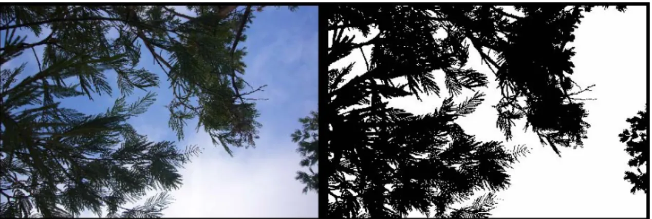
Figure 2: Example of the quantitative field measurements of PPC from upward looking photos. Photos (left) were classified (right) into canopy elements (black) and sky (white). PPC corresponds to the relative

area of canopy elements in the classified photo (0.49 in this example)

The LiDAR-derived PPC estimations were validated using the actual field PPC measurements. To allow this validation, each field site was subdivided into smaller plots of 225 m2. This plot size (15 x 15 m) is equivalent to the area covered by nine photos (3 x 3 photos) and represents a feasible compromise to allow geographic correspondence between both data sets. The average of the LiDAR-derived PPC values for each plot was then compared to the average of the corresponding nine field PPC measurements. A total number of 48 plots were used.

An error matrix was constructed to estimate the land cover classification accuracy. Sixty randomly selected objects were visually classified using both the multi-spectral and the panchromatic bands from the QuickBird image and employed as reference sites. The overall accuracy of the classification and the Kappa statistic were calculated.

Field measurements of streambed width were compared to those automatically obtained from the land cover classification. Since the streambed was frequently hidden underneath the canopy cover of the riparian vegetation, visual assessment of the streambed width from optical information was unreliable. Hence, only field measurements were employed for streambed validation. In the case of the riparian zone width measurements, a set of 34 visually assessed measurements of the riparian zone width was also produced from the multi-spectral and the panchromatic QuickBird bands. They corresponded to 17 sites located along the river where the riparian zone width was measured from both edges of the streambed (right and left hand side of the river) to the external perimeter of the riparian zone. Both in-situ and image-based riparian zone width measurements were compared to the automatically obtained riparian zone widths.

3. Results and Discussion

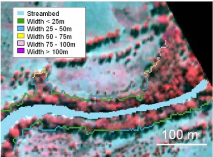
The 0.5 m DTM extracted from the LiDAR data revealed a fairly flat area, with a total height difference of only 25 m (Figure 3a). This information was employed for mapping the streambed of the river according to its geomorphology (Figure 3b). The high precision of this LiDAR-derived streambed map allowed very accurate estimation of the streambed width. Thus, the streambed width measurements obtained from the LiDAR-derived streambed map and the ones measured in the field showed a very high correlation, with a correlation coefficient (r) of 0.98 (RMSE = 1.53).

strong correlation (Figure 4; r = 0.86). Previous studies based on optical information (QuickBird imagery) had revealed that the presence of dense grass cover heavily affects the accuracy of the optical-based PPC estimates (Johansen and Phinn, 2006). In this sense, the use of LiDAR data represents a benefit for the riparian zone analysis.

A TCM estimating the heights of the top of the canopy was also derived from the LiDAR data (Figure 3d). The canopy height ranged from 0 to 41.35 m. This layer of information facilitated the image segmentation and land cover classification. The TCM was useful for tree crown identification and tree height estimation.

Figure 3: LiDAR-derived products: (a) DTM; (b) streambed map (in blue); (c) PPC and (d) TCM. Bright areas correspond to high values for the terrain elevation (a, b), PPC (c) and tree heights (d).

0 0.2 0.4 0.6 0.8 1

0 0.1 0.2 0.3 0.4 0.5 0.6 0.7 0.8 0.9 1

PPC masured from field data

Li

D

A

R

-de

ri

v

e

d P

P

C

Figure 4: Scatter plot of the PPC estimations from the LiDAR data vs the PPC measurements extracted from upward looking photos.

Figure 5: Segmentation levels: (a) LiDAR-derived segmentation and (b) incorporating optical information.

Classification was performed on the final segmentation level using the parameters defined in Table 1. The combined use of LiDAR, spectral and context information allowed accurate identification of the six land cover classes (Figure 6). Fifty-two out of sixty objects were correctly identified as one of the six land cover types, which provided an overall classification accuracy of 88% (Table 2). The Kappa value for the land cover classification was 85%. Riparian vegetation and woodland classes were predicted with the lowest accuracy (63 and 69% respectively), due to the high level of spectral and positional similarity between them in the transitional area between riparian and woodland vegetation.

The LiDAR-derived streambed map was essential for correct identification of vegetation overhang and riparian zone width. A total area of 4.1 hectares of streambed (83.5% of the total streambed mapped for this study area) were located underneath vegetation overhang and would have been impossible to map by means of optical sensors alone. Accurate location of the streambed was also necessary for the riparian zone width estimation. At the same time, the spectral information improved the LiDAR-derived streambed map, which was underestimated in some areas. The original streambed map, derived only from LiDAR data, was missing 4.5% of the final streambed area, mapped after including the QuickBird multi-spectral bands. This confirms the feasibility of combining both sensors for the riparian zone analysis, rather than selecting one over the other.

Figure 6: Land cover classification: (a) Subset of the study area (bands green, red and NIR) and (b) classification result for the same subset.

Table 2: Error matrix of the land cover classification for bare ground (BG), riparian vegetation (RV), woodlands (WL), rangelands (RL), streambed without vegetation overhang (SC) and streambed with

vegetation overhang (VO).

Reference Data User’s

BG RV WL RL SC VO Sum Accuracy

BG 6 0 0 0 0 0 6 100%

RV 0 12 4 0 2 1 19 63.2%

WL 0 0 9 0 0 0 9 100%

RL 0 0 0 7 0 0 7 100%

SC 0 0 0 0 9 0 9 100%

VO 0 0 0 0 0 10 10 100%

Classified Data

Sum 6 12 13 7 11 11 60

Producer’s Acc. 100% 100% 69.2% 100% 81.8% 90.9%

Overall Classification Accuracy = 88.3%

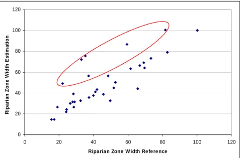
Forty nine measurements of the riparian zone width (five measured in the field and 34 visually assessed from the optical information) were employed for the validation of the riparian zone width assessment. Comparison between the reference and estimated riparian zone widths showed a strong correlation (r = 0.82; RMSE = 13.9), with an overestimation of the automatic assessment in some areas (Figure 8). This overestimation was linked to the presence of woodland areas close to the riparian zone, which were in some cases misclassified as riparian vegetation, and therefore included in the riparian zone width estimation. Because the riparian zone width estimation was based on the land cover classification map, the results relied heavily on the image classification accuracy. Even though establishing the boundary between riparian vegetation and woodlands is challenging (even when it is performed in the field), the overall accuracy of the automatic estimation was high, with an average error of 3.9 m, equivalent to less than 2 pixels in the image.

0 20 40 60 80 100 120

0 20 40 60 80 100 120

Riparia n Zone W idth Re fe re nce

R

ip

a

ri

a

n

Zone

W

idt

h

E

s

ti

m

a

ti

on

Figure 8: Scatter plot of the riparian zone width estimations vs the reference values (i.e. measured in the field and visually assessed from the optical information). The red ellipse shows examples of

overestimation of the riparian zone width.

Conclusions

Several parameters of the riparian zone have been accurately mapped by combining LiDAR and high spatial resolution optical data. These include PPC, streambed with vegetation overhang, streambed without vegetation overhang, the riparian zone with, the streambed width and a land cover map.

Combining LiDAR and high spatial resolution satellite imagery can significantly improve the mapping and assessment of vegetation structure and condition of the riparian zones in Australian tropical savannas. The integration of both sources of information produced an accurate land cover map, despite the high heterogeneity of the riparian landscape. This allowed accurate identification of riparian vegetation, vegetation overhang and the streambed, all of which are commonly used indicators of the riparian zone condition. Moreover, the analysis developed allowed an accurate estimation of the riparian zone width and improvement of the streambed map.

The object-oriented image analysis was appropriate for this type of data integration. This approach also assisted the classification by allowing the incorporation of context information to the classes’ definition. Our results have implications for riparian management in tropical savannas as a tool for monitoring vegetation structure and composition remotely. Further research in this direction should be focused on the estimation and incorporation of other remotely-derived riparian health indicators, such as bank stability and weed mapping.

Acknowledgements

References

Armston, J.D., Denham, R.J., Danaher, T.J., Scarth, P.F. and Moffiet, T., 2008. Prediction and validation of foliage projective cover from Landsat-5 TM and Landsat-7 ETM+ imagery for Queensland, Australia. Journal of Applied Remote Sensing, in review.

Clark, M.L., Clark, D.B. and Roberts, D.A., 2004. Small-footprint lidar estimation of sub-canopy elevation and tree heigth in a tropical rain forest landscape. Remote Sensing of

Environment, 91, 68 - 89.

Congalton, R.G., Birch, K., Jones, R. and Schriever, J., 2002. Evaluating remote sensed techniques for mapping riparian vegetation. Computers and Electronics in Agriculture, 37, 113 - 126.

van Gardingen, P.R., Jackson, G.E., Hernandez-Daumas, S., Russel, G. and Sharp, L., 1999. Leaf area index estimates obtained for clumped canopies using hemispherical photography.

Agricultural and Forest Meteorology, 94, 243 - 257.

Goodwin, N.R., Coops, N.C. and Culvenor, D.S., 2006. Assessment of forest structure with airborne LiDAR and the effects of platform altitude. Remote Sensing of Environment, 103, 140-152.

Johansen, K. and Phinn, S., 2006. Mapping structural parameters and species composition of riparian vegetation using IKONOS and Landsat ETM+ data in Australian tropical savannahs. Photogrammetric Engineering and Remote Sensing, 72, 71 - 80.

Johansen, K., Coops, N.C., Gergel, S.E. and Stange, Y., 2007a. Application of high spatial resolution satellite imagery for riparian and forest ecosystem classification. Remote Sensing

of Environment, 110, 24 - 44.

Johansen, K., Phinn, S., Dixon, I., Douglas, M. and Lowry, J., 2007b. Comparison of image and rapid field assessments of riparian zone condition in Australian tropical savannas. Forest

Ecology and Management, 240, 42 - 60.

Johansen, K., Clark, A., Denham, R., Armston, J., Phinn, S. and Witte, C., 2008. Mapping plant projective cover in riparian zones: integration of field and high spatial resolution QuickBird, Spot-5 and LiDAR data. In Australasian Remote Sensing & Photogrammetry Conference, pp. 12, Darwin (Australia).

Lefsky, M.A., B., C.W. and Spies, T.A., 2001. An evaluation of alternate remote sensing products for forest inventory, monitoring and mapping of Douglas fir forests in western Oregon. Canadian Journal of Forestry Research, 31, 78 – 87.

Lovell, J.L., Jupp, D.L.B., Culvenor, D. and Coops, N.C., 2003. Using airborne and ground-based ranging lidar to measure canopy structure in Australian forests. Canadian

Journal of Remote Sensing, 29, 607 - 622.

Persson, A., Holmgren, J. and Soderman, U., 2002. Detecting and measuring individual trees using an airborne laser scanner. Photogrammetric Engineering and Remote Sensing, 28, 1 – 8.

Popescu, S.C. and Zhao, K., 2008. A voxel-based lidar method for estimating crown base height for deciduous and pine trees. Remote Sensing of Environment, 112, 767 - 781.

Suarez, J.C., Ontiveros, C., Smith, S. and Snape, S., 2005. Use of airborne LiDAR and aerial photography in the estimation of individual tree heights in forestry. Computers &

Geosciences, 31, 253 - 262.

Zimble, D.A., Evans, D.L., Carlson, G.C., Parker, R.C., Grado, S.C. and Gerard, P.D., 2003. Characterizing vertical forest structure using small-footprint airborne LiDAR. Remote