Experimental study on heat transfer enhancement caused by the
flow-induced vibration of a prism inside a channel
F. Sastre, A. Velazquez
*
A B S T R A C T
Keywords:
Heat transfer enhancement Confined laminar flow Passive system Flow induced vibrations
An experimental study, using water as the working fluid, has been performed to analyze whether a pas-sive system based on flow-induced vibration is a feasible option to enhance heat transfer in the laminar confined regime. The experimental setup consisted of a 1.5 m tall vertical channel manufactured on methacrylate (square cross-section of 25 mm x 25 mm) and a tethered square section buoyant prism (10 mm x 10 mm x 25 mm) placed inside the channel. The tethered prism was allowed to move freely (like an inverted pendulum) as a consequence of its interaction with the incoming flow. An aluminum block placed in the channel walls around the prism heated the water with a constant wall temperature of 60 C. The flow Reynolds number (Re) based on the prism cross section length was varied between 80 and 800. Three prisms with three different prism-to-water density ratios (m*) were used in the experi-ments: 0.56, 0.70 and 0.91. The case with the prism anchored to the walls was considered also. Regarding heat transfer, all cases were compared to the reference case which consisted of the clean chan-nel with no prism present. The flow velocity was characterized using a Particle Image Velocimetry System. The electric power supply to the heated walls was recorded and the spatial distribution of water temperature was measured in a transversal plane downstream of the heated walls. It was found that the heat transfer enhancement provided by this system, as compared to the clean channel with no prism pre-sent, was very much dependent on Re. For example, at the lowest Re 80, the improvement on the Nusselt number (Nu) was negligible for all cases. At highest Re 800, the improvement on Nu was 100% for the case of prism-to-water density ratio of 0.91, and 66% for the case of the prism anchored to the walls. This sug-gests that, when thinking of practical engineering applications, passive systems based on flow-induced vibration might represent a feasible alternative, because of its simplicity, to active systems that require a more complex implementation that includes a motor to move the prism. The simplest setup (the prism anchored to the walls) also yields a significant, if smaller, heat transfer enhancement.
© 2017 Elsevier Ltd. All rights reserved.
1. Introduction
Heat transfer e n h a n c e m e n t in confined flows by means of using moving devices is very active area of research. The reason is that, in addition to its relevance as a basic thermal-fluid problem, this R&D
Corresponding author.
E-mail address: [email protected] (A. Velazquez).
field has practical applications for several industrial sectors such as, for example, chemical engineering, energy, food processing, etc. The interest grows larger w h e n e v e r laminar flows are involved because diffusion, that is a slow process, tends to d o m i n a t e heat transfer in this regime. Then, it is of interest to devise n e w methods that target heat transfer e n h a n c e m e n t in this type of flow regimes. A very illustrative example of t h e type of work that is normally carried out in this field can be found in t h e article published by
http://dx.doi.org/10.1016/j.applthermaleng.2017.06.123
Celik et al. [1]. In their 2D numerical study, the authors considered a straight channel with a circular cylinder placed on its centerline. The blockage ratio of the configuration was 1:3. A uniform heat flux was applied to the channel walls while the cylinder itself was assumed to remain adiabatic. The flow Reynolds number (Re), based on the cylinder diameter was 100 and the Prandlt num-ber (Pr) was varied in the range between 0.1 and 100. First, the authors addressed the case of the fixed (unmoving) cylinder so as to compute in this case the frequency of the downstream shed vortices (the reference frequency). Next, they prescribed a har-monic cross flow wise motion of the cylinder and computed the downstream Nusselt number (Nu). The frequencies that they pre-scribed were close to the reference frequency. Their findings for Pr = 5 (that is the case closest to considering water as the working fluid) were as follows: (a) the limiting Nu in the case of the clean channel with no cylinder present was 14, (b) the limiting Nu in the case of the cylinder moving with a frequency of 0.75 times the reference frequency was 17.5 (a 25% improvement), and (c) prescribing frequencies above the reference frequency did not improve heat transfer or even deteriorated it. All this was regard-ing the limitregard-ing Nu in the region far downstream of the cylinder. In the region close to the cylinder, local heat transfer enhancement was larger (close to a 50% of improvement). Another numerical 2D study has been reported by Fu and Tong [2]. In this case, the authors considered three different blockage ratios, 1:8, 1:4, and 1:2 for different combinations of frequency and amplitude of the cylinder motion at Re 500 based on the channel height (the work-ing fluid was air). In yet another study, Fu and Tong [3], performed comparisons in terms of the average Nu. In a short channel section downstream of the cylinder, heat transfer associated to the moving cylinder improved by a factor of 31% the heat transfer rate of the clean channel (no cylinder present). When averaging the Nu over the whole channel, the improvement was 23%. So these conclu-sions are qualitatively and quantitatively similar to those already mentioned of Celik et al. [1].
Yang and Chen [4] have presented another 2D numerical study in which four heated blocks were attached to walls of a channel in which a cylinder was moving with prescribed frequencies and amplitudes. The aspect ratio of the blocks was 1:4 and Re was higher than in previous references (800-8000 based on the cylin-der diameter). The working fluid was also air. Depending on the selected frequencies and amplitudes of the cylinder motion, heat transfer rate improvements (defined as the space-time averaged Nu in the case with cylinder versus the case without cylinder) ran-ged from 8% to 17%. The case in which the cylinder itself is the heated element and its motion is used to enhance heat transfer from the cylinder to the surrounding fluid has also been studied extensively. For some examples, the interested reader is referred to the works of Ghazanfarian and Nobari [5], Nobari and Ghazan-farian [6] and Pottebaum and Gharib [7].
In all the references mentioned previously, the cylinder motion was prescribed (an active system). It means that in an actual engi-neering situation some kind of motor with an associated mecha-nism has to be used. This, by itself, might be difficult, in particular when dealing with mini/micro systems. It might also be prone to suffer from functioning problems such as leakages, motor failures, etc. In this context, the objective of the present arti-cle is to study whether a very simple passive system in which the prism motion is self-generated and self-sustained might provide some acceptable enhancement of the heat transfer rate from the channel walls into the fluid. Specifically, this self-sustained motion occurs because of the interaction between the incoming flow and the cylinder (the phenomenon called flow induced vibration). In this way, the system design and actuation is much simpler (it is, for instance, water tight) which may facilitate its actual use in industrial applications. Regarding the basic fluid mechanics
aspects of this problem, the reader is referred to the isothermal experimental studies published by Reyes et al. [8] and Reyes et al. [9]. In these two studies, detailed Particle Image Velocimetry (PIV) based analysis were presented on the flow topology past a fixed square section prism and a free prism allowed to move unhindered in the crossflow direction inside a square section chan-nel. The different flow regimes were analyzed and it was found that, depending on the Re and on the body to fluid density ratio (the body was buoyant), both periodic and chaotic flow conditions could be observed. Now, in the present article, the objective is to move one step ahead by way of including thermal effects so as to find out whether these flow regimes might enhance the mixing of a passive scalar such as temperature.
Regarding to the article organization, the experimental set-up is described first. Then, the experimental campaigns are defined and the results are presented and discussed. Finally, conclusions are presented.
2. Description of the experimental setup and measurement systems
The experimental setup had the form of a closed loop circuit, see Fig. 1. The main parts of the setup were: the test channel, the test section, the power supply unit, three tanks, a flow meter, a pump, and a radiator to prevent the recirculating water from over-heating (before entering the main tank, water temperature was monitored to be constant at the level of 25 C).
2.1. The test channel
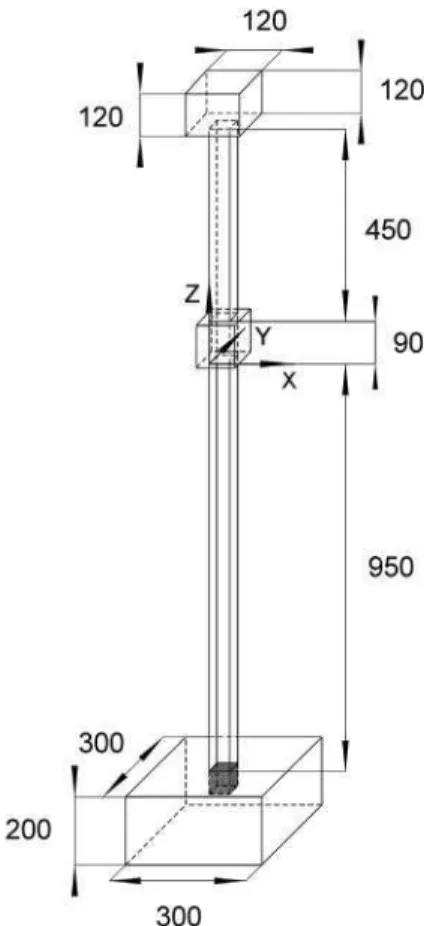
It was manufactured in methacrylate and it was placed verti-cally. Its square cross section was 25 mm x 25 mm. Its total height was 1490 mm. The thickness of the channel walls was 10 mm. The channel was inserted into a large primary tank where the flow was homogenized. To achieve further homogenization, so as to shorten as much as possible the hydrodynamic entrance length, a honey-comb section was inserted at the entrance of the test channel (the inflow section). The outflow section discharged into a sec-ondary tank where the water level remained constant; the idea being to avoid pressure fluctuations in the test section of the chan-nel. A view of the channel together with information on the loca-tion of the origin of coordinates and all associated distances is presented in Fig. 2.
2.2. The test section
The heated test section was 90 mm long and it was located mid-way along the channel (see Fig. 2). It consisted of a hollow alu-minum block, where the tethered prism was inserted, located a distance 950 mm away from the channel inflow section (see Fig. 2). A close-up view of this test section is shown in Fig. 3.
Secondary tank
Test section Aluminium block
Power supply
Auxiliary tank
0
Primary tank
\Test
channel
Honeycomb Flow direction
Flow meter
Pump
Heat exchanger
Fig. 1. Sketch of the experimental setup.
120
120
Vm
300
120
450
90
950
200
300
Fig. 2. View of the test channel and primary (bottom) and secondary (top) tanks. The heated section (90 mm height) can be observed midway along the channel where the origin of coordinates is placed. Distances are expressed in mm.
powered with a square wave, controlling its duty cycle using a relay, so as to maintain a uniform wall temperature. Table 1 shows the time-averaged temperatures measured by the 10 thermocou-ples (Tl to T10), and both the standard and maximum temperature deviations for the case of the fixed (unmoving) prism for some rep-resentative Re. The coordinates of the inserts were the thermocou-ples were placed are also given in Table 1 (notice that some coordinates are negative and some other larger than 25 mm because these thermocouples were placed inside the aluminum walls and they were not in contact with the fluid). The thermocou-ples were of the Tcdirect brand and they measured with an uncer-tainty of ±0.5C. They were connected to a NI9214 data acquisition system with a sensibility of ±0.02C. At the lowest Re, the maxi-mum spatial temperature deviation between thermocouples was of the order of 1 C. This deviation was of the order of 45 C at the highest Reynolds number.
Nine additional temperature measurement points were placed in a plane located 20 mm downstream of the aluminum block (60 mm downstream of the prism), see Fig. 3, to measure the spa-tial distribution of water temperature inside the channel. To min-imize flow disturbances, these temperatures were acquired one by one using a sequential procedure. Specifically: each single thermo-couple was inserted through the channel wall into the flow field, was allowed to measure and, then, retrieved. The inserts were sealed with plastic material to prevent leaking. The process was sequentially repeated for all 9 measurement locations. Fig. 4 shows the actual spatial locations where the thermocouples were inserted. The view is from the top of the channel down towards the test section; this why the prism (shaded in grey color) is also seen in the figure. Finally, an actual photograph of test section together with some of the prisms used in the experiments are pre-sented in Fig. 5.
Regarding the prisms, they were hollowed out when manufac-tured so as to achieve different density ratios, m*. Specifically, three prisms with the following m* were manufactured: 0.56, 0.70 and 0.91.
2.3. Auxiliary systems
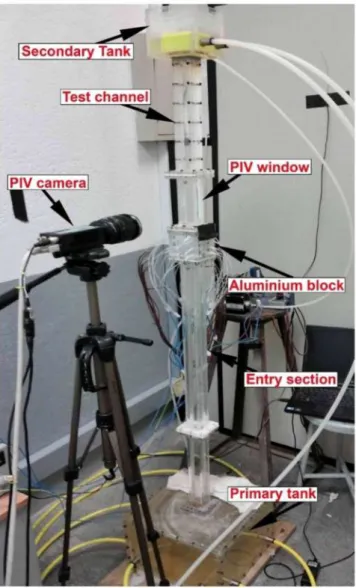
The flow meter was an electromagnetic Siemens Sitrans FM MAGI 100 equipped with a Sitrans FM MAG5000 transmitter. The measurement range was from 0 to 5 1/min and the uncertainty was ±5%. The pump was an ITT Totton centrifugal with a magnetic drive DC15/5. An overview picture of the whole experimental setup is presented in Fig. 6.
2.4. The Particle Image Velocimetry (PIV) system
This PIV system was from Dantec Dynamics. Flow illumination was achieved with a pulsed Nd:YAG 800 mj Laser. The time lapse between two laser pulses (needed to collect a single sample) was
Thermocouples Thermocouple plane Aluminium block,
\
Test section
Aluminium block Methacrylate Tether
Table 1
First three columns: coordinates (in mm) of the inserts where the thermocouples were placed. Other columns: measured time-averaged temperature (C) of the 10 thermocouples inserted into the aluminum block (Tl to T10) for some representative Re. Average temperature, T„v, standard deviation, Tst, and the maximum deviation, ATmax, are also included.
Re Tl T2 T3 T4 T5 T6 T7 T8 T9 T10 Tav Tst
A i max
X 12.5 12.5 12.5 12.5 26.0 -1.0 26.0 -1.0 26.0 -1.0 y -1.0 26.0 -1.0 26.0 12.5 12.5 12.5 12.5 12.5 12.5 z 70.0 70.0 25.0 25.0 70.0 70.0 45.0 45.0 20.0 20.0 80 T(C) 58.8 58.7 58.9 58.7 58.4 58.5 59.5 59.6 58.9 59.5 59.0 0.4 1.2 133 57.8 57.8 58.2 58.0 57.3 57.4 58.8 58.7 58.2 58.5 58.1 0.5 1.5 260 58.6 58.1 58.9 58.5 57.1 57.5 59.0 59.2 58.7 59.1 58.5 0.7 2.1 360 59.3 58.8 59.4 59.2 57.5 57.4 59.3 59.5 59.4 59.8 59.0 0.8 2.3 466 58.9 58.4 59.8 59.4 57.0 56.9 59.1 59.0 59.8 60.0 58.8 1.1 3.2 733 53.1 52.7 55.0 54.7 50.8 50.7 53.2 53.4 55.1 55.4 53.4 1.7 4.7
12.5
7.5 412.5
Fig. 4. Position of the 9 points (located downstream of the aluminum block) where
water temperature is measured. The view is from the top of the channel into the test section. The prism is shaded in a darker grey mesh. Measurements are expressed in mm.
5 ms. At the maximum flow velocity used in the experiments, a particle would travel 0.3 mm between pulses that is a distance much smaller than the problem characteristic length of 10 mm (the prism cross section length). The camera was a Dantec
Dynam-ics Flow Sense 2ME with a resolution of 1600 x 1200 pixels. The lens was a Zeiss Makro-Planar T* 2/50 mm ZF. Flow seeding was performed with 10 urn hollow glass spheres (HGS-10). Dantec Dynamics Studio software was used to synchronize image captur-ing and flow illumination, and to perform the analysis. The size of the interrogation areas was 50 mm x 25 mm. These areas were subdivided into smaller areas by the analysis software to achieve convergence in the re-computation process of the flow field. It was estimated that the spatial resolution of the flow field was of the order of 1 mm that should be enough to capture the large flow structures whose size was of the order of the prism cross-section length (10 mm). The sampling frequency was 15 Hz. Afterwards, it was found that the relevant flow frequencies were of the order of 1 Hz, so the temporal resolution of the experimental setup was adequate to capture the relevant flow features.
3. Definition of the experimental campaigns
Six different experimental campaigns (EC) were carried out in the present study. They were labeled EC #1 to EC #6. Their defini-tion is as follows:
• EC # 1 . Clean channel with no prism present. Isothermal walls. Re, based on a characteristic length of 1 cm (the prism cross sec-tion length in the cases where the prism is present) equal to: 80, 160, 200, 240, 320, 400, 600, and 800. The lowest volume flow
Fig. 5. Pictures of the test section (notice that the outside of the aluminum block is isolated with low thermal conductivity methacrylate panels) and two prisms with the
Fig. 6. Overview of the experimental setup.
rate corresponding to Re 80 was 0.268 1/min (average inlet velocity equal to 0.007 m/s). The largest volume flow rate corre-sponding to Re 800 was 2.68 1/min (average inlet velocity equal to 0.070 m/s).
• EC #2. Clean channel with no prism present. Walls heated to the temperature level specified in Table 1. The Re range equal to that of EC # 1 .
• EC #3. Channel with prism anchored to the walls (no prism motion allowed). Isothermal walls. Re (based on the prism cross section length of 1 cm) equal to: 80, 106, 133, 160, 200, 240, 260, 280, 300, 320, 360, 400, 466, 533, 600, 666, 733, and 800. • EC #4. Channel with prism anchored to the walls (no prism motion allowed). Walls heated to the temperature levels speci-fied in Table 1. The range of Re equal to that of EC #3. • EC #5. Channel with tethered prism placed inside and allowed
to move freely. Isothermal walls. The range of Re equal to that of EC #3. Three different prisms to water density ratios were considered for each case: 0.56, 0.70 and 0.91.
• EC #6. Channel with tethered prism allowed to move freely. Walls heated to the temperature levels specified in Table 1. The range of Re equal to that of EC #3. Three different prisms to water density ratios were considered for each case: 0.56, 0.70 and 0.91.
Accordingly, the total number of experimental cases addressed in the study was 160 (EC # 1 : 8 cases, EC #2: 8 cases, EC #3: 18
cases, EC #4: 18 cases, EC #5: 54 cases, EC #6: 54 cases). A limited set out of these 160 cases was selected for the repeatability tests. The outcome of these repeatability tests will be described in the following sections.
4. Results
4.1. EC #1 campaign
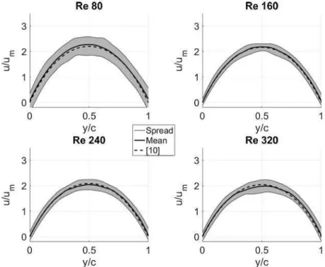
This campaign could be considered as the setup calibration campaign because results were compared to those obtained theo-retically by [10] for laminar flow in a square section channel. This is observed in Fig. 7 where the average value of the 100 measured velocity profiles, their maximum spread, and the theoretical profiles are presented. Out of the whole set of results, four Rey-nolds numbers (80, 160, 240, and 320) were selected for illustra-tion purposes in Fig. 7. In these cases, the flow is hydrodynamically developed before reaching the measurement section so that comparison with the theoretical results of [10] can be consistently performed.
Regarding the spread of the measurements, see the gray shaded bands in Fig. 7, the histogram presented in Fig. 8 shows a typical distribution of the 100 centerline velocity measurements around the mean (the case of Re 160 has been chosen for illustration purposes).
4.2. EC #2 campaign
This case is like the previous one but for the fact that the alu-minum block is heated up to a constant temperature of 60 C. The counterpart of Fig. 7 for this case is presented in Fig. 9. There, it could be observed that at the lower Re, buoyancy dominates the velocity profiles (notice the high velocity plumes ascending close to the walls at y/c = 0 and y/c = 1). As the Re increases, this effect losses its importance until the convection from the main body of fluid dominates again the velocity profile (except in a small region close to the walls) at Re 320.
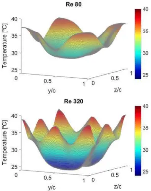
The temperature information obtained from the thermocouples inserted in the flow field in the transversal plane located 20 mm downstream of the aluminum block was processed, using a nearest neighbor algorithm [11] together with symmetry considerations, to reconstruct the temperature field in that plane. An example of this reconstruction for Re 80 and Re 320 is presented in Fig. 10. These temperature planes will be used in the next sections to assess the degree of mixing in the flow field.
The Nusselt number, Nu, in this thermal case is defined as: Nu = hL/kfiim where h, L, and kfnm are the convection heat transfer coefficient, the characteristic length, and the water thermal con-ductivity at the film temperature. The characteristic length for Nu was taken to be the hydraulic diameter of the channel (0.025 m). The film temperature was defined as:
T 2 ' 'w a H M l
'/ilm = 2 *• '
where Tin, Tout, and TwaII were inlet, outlet, and wall temperature respectively. !,„, and TwaII were measured directly. The fluid temper-ature downstream of the heated section, Tout, was computed by means of an energy balance: Qin +HP = Qout, where Q,„ and Q_out where the thermal energy per unit time entering and leaving the test section respectively, and HP was the measured electrical heat-ing power. Then, h was computed by performheat-ing the followheat-ing balance:
Re 80
Re
160Fig. 7. Average value of the 100 measured velocity profiles for Re 80,160, 240 and 320 (solid lines), their maximum spread (gray bands), and the theoretical profiles (dashed
lines).
50
40
30
20
10
0
• PIV values —Mean value
2.1 2.2 2.3 2.4 2.5
u/u
Fig. 8. Histogram of the 100 centerline velocity measurements around the mean for Re 160.
where Ahv, was the heated wall area. Once h and 7);lm were obtained
in this way, the Nusselt number was computed.
UP (i.e.: the thermal power supplied to the flow of water to keep the aluminum block at a constant temperature of 60 C) and Nu as a function of Re are presented in Table 2. There, it could be observed that this power supply was nearly constant in the range from Re 80 to 600 (Re 200 to 1500 if based on the channel hydraulic diameter) which suggests that Nu is constant (as it could be observed in Table 2). This is in line with the well-known theoretical result [12] that states that the Nu in a heated square/rectangular channel in the laminar regime does not depend on the Re. It is to be noted that the Nu as given in reference [12] for a square section channel in the laminar regime is 3.6. However, that result is for a hydrody-namically and thermally developed flow, and with heat transfer being applied along all channel walls, which is not the case addressed in the present study; thereby the differences in Nu
values. Given the uncertainty associated to the measurements of the thermocouples and the power unit, it was estimated that the typical uncertainty in the computed Nu was of the order of ±5%.
4.3. EC #3 and EC # 5 campaigns
These two campaigns correspond to the isothermal case with prism present. In particular, in EC #3 the prism is anchored to the channel walls, while in EC #5 it is tethered and allowed to move. Flow characterization was carried out using the PIV system described in Section 2.4. The sketch of the actual PIV interrogation window integrated into the experimental result is presented in Fig. 11. It could be observed that this window is located 60 mm (6 diameters) downstream of the prism. This is so because the prism is enclosed in between solid aluminum walls that do not allow for PIV sensing. This means that the flow structures that can be actually sensed are, at least, at a distance of six diameters away from the prism. Furthermore, given the fact that the flow is highly confined, these structures are likely to be smeared out as a consequence of the strong interactions taking place and the vis-cous effects enhanced by the nearby walls.
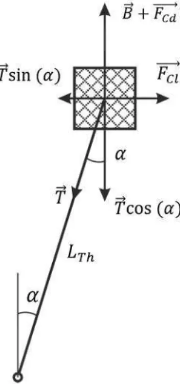
The solid to fluid mass ratio m* influences the prism motion and, as a consequence, the flow field topology downstream of the prism and the associated mixing. This is apparent when the prism equations of motion are written, see Fig. 12.
The two equations of motion in the limit a <C l(cos(a) e* l,sin(a) e* a) are:
B + Fa = T
r T d ar
Fa-T(x = mp—IL.Th dt
(3)
(4)
where B, FCd, T, Fa, a, mp,t, In, are buoyancy force, drag force, tether
tension, lift force, angle of motion, prism mass, time and tether length. Introducing T from Eq. (3) into Eq. (4) yields:
Fa- (B + Fcd)x = mp—j.
Re 80
Re 160
Fig. 9. Counterpart of Fig. 7 for the case of heated walls (no theoretical results are available in this case).
Re 80
Table 2
Measured electric power supply and Mi as a function of
Re for experimental campaign EC #2.
Fig. 10. Reconstructed temperature field in a plane located 20 mm downstream of
the aluminum block for Re 80 and 320.
That is: the buoyancy force B, that depends directly on the solid to fluid mass ratio m*, enters the prism equation of motion in such a way that the lower m* the larger B, and, therefore, the larger the restoring force Tsin(oc) e* Toe. For the cases considered in the exper-iments, the maximum values of a obtained were of the order of 0.05 rad <c 1 rad, so the approximate Eqs. (3)-(5) hold to a reason-able degree of accuracy. In practice, different values of m* could be
Re
80 160 240 320 400 600
H p ( W )
214 215 214 214 219 220
Nu
32.0 32.0 31.9 31.8 31.8 31.7
obtained using different materials for the manufacturing of the prism although, as described in Section 2.2, the method chosen is the present study was to use appropriately hollowed out cylinders of the same material.
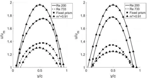
The two horizontal dashed lines A and B in Fig. 11 above indi-cate the two specific locations that have been used for analysis purposes. In particular the downstream velocity has been time averaged and it is presented in Fig. 13 along these two lines for Re 200 and Re 733 for both the fixed prism and the moving prism with m* = 0.91. According to the results presented in reference [9] the case of Re 200 corresponds to the flow regime in which the prism undertakes low frequency and moderately high amplitude oscillations with a well-defined Karman-type wake, while Re 733 corresponds to a chaotic regime.
Fig. 11. Sketch showing the PIV interrogation window in the channel.
Fig. 12. Forces acting on the prism.
one would think that the large moving structures generated by the oscillating prism would require a longer channel length to attain their limiting state. However, this question is somewhat out of the main focus of the present article and it will be addressed by the authors in a future work. In the chaotic regime (Re 733) the behavior is just the opposite: the flow generated by the fixed prism is closer to its limiting PoiseuiUe type limiting state. The results of section B (located closer to the prism at a distance of 6.5 diameters in the downstream direction) are consistent with the results obtained for section A.
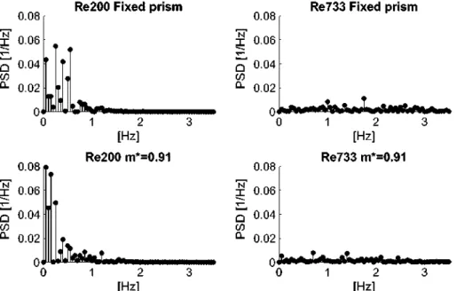
The time averaging process was carried out at a frequency of 15 Hz during 20 s. That is: 300 time frames were used to generate each of the curves presented in Fig. 13. The power spectral density plots of the points of each curve located at the channel centerline (y/c = 0.5) are presented in Fig. 14. It could be observed that at Re 200 the significant frequencies for the fixed prism were below 1 Hz. For the case with m* = 0.91, a distinct frequency appears at 2 Hz. This also supports the idea that the sampling carried out at 15 Hz was consistent with the characteristic frequencies of the phenomena itself. In the case of Re 733, the PSD plots show the typical flat appearance of the chaotic flow.
4.4. EC #4 and EC #6 campaigns
The counterpart of Fig. 13 for the thermal cases is presented in Fig. 15. It could be observed that, in this case, the flow profile at Re 200 is still dominated by buoyancy since the velocity in the region close to the walls is markedly higher than in the channel center-line. At Re 733 the opposite happens: velocity at the centerline is higher than in the near wall region. The PSD plots of these cases are presented in Fig. 16.
5. Discussion
The present work focuses on the question of whether a passive system whose motion is caused by fluid-body interaction is able to improve heat transfer significantly in practical engineering appli-cations. In this view, Fig. 17 shows the summary of results regard-ing the electric power supply to the aluminum walls as a function of Re and m* (including the fixed prism case) for constant wall tem-perature. For any given m*, the supplied power was increased along with Re to keep a constant aluminum wall temperature. The maximum available power delivered by the DC unit was 315 W. This threshold level was achieved at Re 320 for m* = 0.91 and at Re 520 for m* = 0.56. For the case of the fixed prism the threshold level was also reached at Re 520.
To quantify the different heat transfer rates, Nu as a function of Re and m* has been computed and the results are presented in
Table 3. It could be observed that Nu grows along with Re and that the configuration that yields the higher Nu is the one with m* = 0.91. These results correlate with the following expression: Nu = 23.3lReomm*022. As compared to the results presented in Table 2 (the clean channel) the maximum improvements are of the order of 36%. It could be argued that this improvement comes at the expense of a higher pressure drop and, therefore, of a higher pumping power. This is true; however, it has been estimated that the pressure drop caused by the prism is negligible compared to the hydrostatic pressure difference in the vertical channel. In par-ticular, the numerical simulations of Martin and Velazquez [13] show that for a fixed prism inside a channel with the same geom-etry and blockage ratio the total drag coefficient is 4.8 at Re = 100. This yields a dimensional pressure drop of about 0.25 Pa that is not feasible to measure with standard laboratory equipment (mea-surement uncertainties of ±50 Pa are typical for this type of pres-sure sensors).
— Re 200 - - Re 733
• Fixed prism A m*=0.91
— R e 200 - - Re 733
• Fixed prism A m*=0.91
Fig. 13. Time averaged "z" velocity profiles for Re 200 and 733. Results are presented in planes z = 115 (left) and z = 140 (right) for the fixed prism and, also, for the case with
m" = 0.91.
0.08
Re200 Fixed prism
N 0.06
— 0.04 Q a. 0.02
0
0.08
N 0.06
— 0.04 Q a. 0.02
0.08
Re733 Fixed prism
[[^BrfmjBJfUli . -m.
N
Q CO Q .
0.06
0.04
0.02
1 [Hz]
Re200 m*=0.91
0
0.08
1 2 [Hz]
Re733 m*=0.91
JkwM*
N J . T 1—'
u m a.
0 06
0 04
0.02
0 1 0 1 2
[Hz] [Hz]
Fig. 14. Power spectra density plots of the downstream velocity in the channel centerline for the isotherm fixed prism at Re 200 and Re 733.
1.4
1.2
rs 0.8
0.6
0.4
0.5 y/c
— R e 200
- - Re 733 • Fixed prism A m*=0.91
1
0.08 ? 0.06
Q 0.04
CO °- 0.02
Re200 Fixed prism
i.
1
0.08
[Hz] Re200 m*=0.91
0.08 Re733 Fixed prism N
T
T—
n
CO LL
0.06
0.04
0.02
0 JM<M*™<^Jw*w8ilMftiWlM»t«»
0.08
1
[Hz] Re733 m*=0.91
N
-^—
n
CO LL
0.06
0.04
0.02
0 1 2 3
[Hz]
Fig. 16. Counterpart of Fig. 12 but considering now the thermal case.
350 r
300
8
CL
250
200
• Fixed prism A m*=0.91
• m*=0.70 T m*=0.56
/ • ^ — * — * — * — ~
100 200 300 400 500 Re
600 700 800
Fig. 17. Electric power supplied by the DC unit to the aluminum walls (heat transfer to the fluid) as a function of Re and m" for constant wall temperature. The case of the fixed prism is also included for comparison purposes.
lowest m*. As it can be observed in Fig. 16, this behavior is consis-tently observed for Re up to 400. This suggests that not all types of prism motion improve heat transfer as compared to the case of the fixed prism. In fact, the case with m* = 0.56 yields a heat transfer consistently smaller than the case with the fixed prism all over the discussed Re range. The authors think that this is related with
the flow topologies generated by the prism motion and their inter-action with the buoyant plumes that originate at the solid alu-minum walls. Ideally, the best study option for this effect would be to perform a PIV based analysis of these structures, but this appears to be impossible owing to the fact that the aluminum walls are opaque. Then, the only feasible approach seems to be a CFD based one that is out of the scope of this work (it will be addressed by the authors in a future work). These experimental results are, nevertheless, somewhat unexpected because, in a sense, it would be tempting to regard a fixed prism as a system characterized by an infinite buoyant force that leads to an infinite restoring force that suppresses all possible motion. Within this perspective, the fixed prism could be considered as the asymptotic limit of a sequence of prisms in which the buoyant force keeps growing. However, in view of the observed experimental results this does not appear to be the correct approach. Possibly, what happens is that the presence of an additional equation of motion for the cases in which the prism moves changes the system dynamics completely.
Fig. 18 presents the time average of 300 PIV frames (20 s of experiment) for Re 200. Both the dimensionless stream-wise U velocity and the cross-wise velocity V are plotted for EC #4 (the thermal fixed prism) and EC #6 (the thermal moving prism with m* = 0.91). The two upper subplots (stream-wise velocity) show a similar topology: the actual values of the time-averaged velocity might be slightly different but the global behavior is basically the same. However, the two lower subplots that depict the cross-wise velocity are different. In particular, the left one (fixed prism) shows that the average cross-wise velocity near the channel walls is small: it has different shades of green color that means that this
Table 3
Nu as a function of Re and m" for the constant wall temperature case.
fie
80
133 160 200 240 300 360
m 30.7 31.7 31.1 30.8 31.1 33.6 36.5
= 0.56 m
32.6 33.2 33.3 32.6 33.7 38.3 39.6
= 0.70 m =0.91
33.3 32.0 32.8 34.7 36.6 40.0 43.2
EC #4 U/U EC # 6 m*=0.91 U/Umean
0.05
0.05
EC #6 m*=0.91 V/U
0.05
-0.05
Fig. 18. Time-averaged PIV plots of the dimensionless stream-wise (U/Umean) and cross-wise (V/Umean) velocities at Re 200, for EC #4 (the thermal fixed prism) and EC #6 (the
thermal moving prism with m" = 0.91).
average velocity value is around zero (see the color bar to the right of the plot). On the other hand, see the lower right subplot, the case with the moving prism shows that the time-averaged cross wise velocity is positive the vicinity of the channel left wall (it has shades of yellow-orange1 color) that means that its direction is from
the left wall towards the channel centerline. At the same time, it could be observed that the time-averaged cross-section velocity is negative in the vicinity of the channel right wall (it has shades of blue color) that means that, again, its direction is from the (right) wall towards the channel centerline. That is, the presence of the moving prism modifies the topology of the time-averaged cross wise velocity in the sense that it promotes motion from the walls towards the channel centerline, thereby promoting the transport of heat from the walls into the bulk flow. The fact that this cross-wise velocity is small when compared to the stream-wise velocity imposed a limit on the additional amount of heat that can be actually transferred from the channel walls into the main body of fluid.
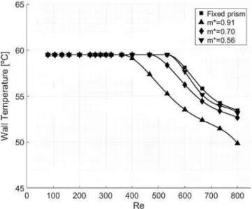
Once the maximum power level was reached, further incre-ments of Re led to a decrease in the wall temperature because of the growing heat transfer rate. This can be observed in Fig. 19 where the average wall temperature is presented as a function of Re and m* (including, also, the fixed prism case). The actual mea-surements of the 10 thermocouples as function of Re for the cases of m* = 0.91 and fixed prism are presented in Table 4 for four rep-resentative Re (106, 200, 260, and 733). At the highest Re, the
lar-gest temperature difference in the aluminum walls was 4 C. It is also worth noting that the larger the Re, the more similar are the results of m* = 0.70, m* = 0.56 and fixed prism, while the wall tem-perature for m* = 0.91 keeps consistently lower. Again, this
sug-1 For interpretation of color in Fig. 18, the reader is referred to the web version of
this article.
400 500
Re
Fig. 19. Average aluminum wall temperature as a function of Re and m" once the
Table 4
Detailed temperature measurements (C) of the 10 thermocouples (Tl to T10) inserted into the aluminum walls as a function of Re for the fixed prism and the case with m" = 0.91.
Tl T2 T3 T4 T5 T6 T7 T8 T9 T10 i?el06 Fix. 57.9 57.8 58.3 58.1 57.4 57.5 58.8 58.8 58.3 58.7
m" = 0.91
60.4 60.0 59.4 59.2 59.4 59.9 60.6 60.8 59.3 59.9 i?e200 Fix. 60.3 59.9 59.6 59.3 59.3 59.5 60.5 60.5 59.5 59.8
m" = 0.91
59.0 58.5 58.8 58.5 57.9 58.1 59.4 59.3 58.6 59.3 i?e260 Fix. 58.6 58.1 58.9 58.5 57.1 57.5 58.9 59.2 58.7 59.1
m" = 0.91
60.5 59.5 60.0 59.7 58.8 59.1 60.1 60.2 59.8 60.5 i?e733 Fix. 53.1 52.7 55.0 54.7 50.8 50.7 53.2 53.4 55.1 55.4
m" = 0.91
51.6 51.0 53.0 52.8 49.1 49.4 50.4 50.3 53.0 53.7 Table 5
Nu as function of Re and m" for the constant wall heat transfer case.
Re m = 0.56 m = 0.70 m =0.91 Fixed prism
533 600 666 733 800 41.3 42.1 44.3 44.7 46.9 44.0 47.0 48.5 50.6 53.0 47.4 50.8 51.8 54.2 59.4 44.0 46.1 47.7 49.1 50.9 Table 6
RMS of the dimensionless water temperature for the case of constant wall temperature as a function of Re and m".
m =0.56 m =0.70 m =0.91 Fixed prism
i?e80 i?el33 i?el60 i?e200 i?e240 i?e300 i?e360 3.51 4.22 4.11 3.89 3.37 1.39 1.19 3.82 4.60 4.56 3.11 2.65 1.60 1.25 3.67 4.33 3.96 2.51 2.63 1.41 0.94 2.97 4.24 3.53 3.36 2.59 1.98 1.80 Table 7
RMS of the dimensionless water temperature for the case of constant wall heat transfer as a function of Re and m".
m =0.56 m =0.70 m =0.91 Fixed prism
i?e533 i?e600 i?e666 i?e733 i?e800 0.74 0.76 0.55 0.48 0.60 0.72 0.70 0.51 0.47 0.49 0.47 0.52 0.46 0.46 0.31 1.30 0.72 0.60 0.56 0.52
gests that the dynamics of the system influences significantly the heat transfer rate. In this regard, the behavior of the cross-wise time averaged velocity in the vicinity of the walls is qualitatively similar to the one shown in Fig. 18.
Nu as a function of Re and m* has also been computed for the cases presented in Fig. 19 and the results are shown in Table 5. These results correlate with the following expression: Nu = 4.07Re0A0m*037. As compared to the clean channel case (see Table 2) the improvement on Nu is about 100%. As compared to the fixed prism case (see Table 5) the improvement on Nu is about 20%
Another aspect to be analyzed is the spatial variation of temper-ature on the plane where the thermocouples were inserted into the fluid. To quantify this variation, the rms of the reconstructed 2D dimensionless temperature distribution downstream of the prism has been computed (following the procedure illustrated in Fig. 10) and the results are presented in Tables 6 and 7 for the cases of constant wall temperature and constant wall heat transfer cases respectively. When looking at the results of Table 6, it could be
observed that from Re 200 onwards the rms of the temperature sig-nal for m* = 0.91 case is consistently lower than in the other cases. This suggests that local mixing is achieved more efficiently in this particular case of m* = 0.91 which leads to a better global mixing and higher Nu, as it is indeed the case. That is, the results presented in Table 6, that were obtained processing local temperature data, support the results of Fig. 17 that were of a global nature. For the constant wall heat transfer case, see Table 7, the trend is the same and the rms of the temperature signal for m* = 0.91 is the lowest of all.
6. Conclusions
The Reynolds number based on the prism cross section length (10 mm) was varied between 80 and 800. Three prism-to-water density ratio were considered: m* = 0.56, 0.70 and 0.91. The clean channel case and the case with a fixed prism were also addressed for comparison purposes. The conclusions of the study could be stated as follows.
• In the configuration that has been studied, the presence of either a fixed or a moving buoyant prism always improved the heat transfer rate as compared to the clean channel case. In the case of the moving prism, the improvement on Nu was as high as 100%. In the case of the fixed prism, the maximum improvement was 66%.
• The reason for the improvement could be associated to the fact that both the fixed and the moving prisms modify substantially the flow topology in a way so as to enhance mixing. It should be noted that the length of the wall that was heated was 90 mm while the prism cross section length was 10 mm. If the heated portion of the wall is longer, it is expected that the flow tends to attain its limiting Poiseuille type behavior and the enhance-ment effect should die away further downstream of the prism. • Not all moving prisms generated heat transfer rates higher than the case of the fixed prism. In fact, the case with m* = 0.56 (the lowest one) consistently yielded the lowest Nu values. This sug-gests that not all types of prism motions improve heat transfer in the same way. The reason, again, could be ascribed to the dif-ferent flow topologies that appear associated to the difdif-ferent values of m*.
• For the configuration and parametric range presented in this study, the best configuration was the one with m* = 0.91. • The 2D temperature profiles in the channel sections
down-stream of the moving prism have been analyzed and it has been found that the lowest rms correspond to the case with m* = 0.91. This, again, supports the idea that this specific config-uration promotes mixing in a way that is more efficient than others with lower m*, and also more efficient than the fixed prism case.
• From the fundamental Fluid Mechanics point of view, the pre-sent study poses some questions that will need further analysis in the future. One of these is why depending on the value of m*, the prism in self sustained motion may either improve or dete-riorate the heat transfer as compared to the fixed prism. • From the engineering applications context, all that has been
presented suggests that when devising practical applications, these types of passive configurations, that are conceptually very simple, might have some advantages over active systems when dealing with mixing at low Reynolds numbers. Specifically, an active system needs the presence of a motor with independent power supply that moves impeller type (or other) devices. This,
on one hand, leads to a more complex system and, on the other, requires some mechanical connection between the external motor and the internal propeller-like device which might cause liquid leakage outside the channel (pipe). On the other hand, the external motor can control the amount of mechanical work that can be put into the fluid so the mixing can be more efficient. Thereby, the final selection of the system, either active or pas-sive, might be the outcome of a compromise between system complexity and actual efficiency. In any case, the present study shows that the passive option could be, in some cases, an acceptable solution in terms of simplicity and efficiency.
Acknowledgements
The authors were funded by the Spanish Ministry of Economy and Competitiveness (Ministerio de Economia y Competitividad) under research contract DPI2013-45207. They gratefully acknowl-edge this support.
References
[1 ] B. Celik, M. Raisee, A. Beskok, Heat transfer enhancement in a slot channel via a transversely oscillating adiabatic circular cylinder, Int. J. Heat Mass Transf. 53 (2010) 626-634.
[2] W.S. Fu, B.H. Tong, Effects of eccentricity of cylinder and blockage ratio on heat transfer by an oscillating cylinder in a channel flow, Int. Comm. Heat Mass Transf. 30 (2003) 401-412.
[3] W.S. Fu, B.H. Tong, Numerical investigation of heat transfer of a heated channel with an oscillating cylinder, Numer. Heat Transf. 43 (2003) 639-658.
[4] Y.T. Yang, C.H. Chen, Numerical simulation of turbulent fluid flow and heat transfer characteristics of heated blocks in the channel with an oscillating cylinder, Int. J. Heat Mass Transf. 51 (2008) 1603-1612.
[5] J. Ghazanfarian, M.R.H. Nobari, A numerical study of convective heat transfer from a rotating cylinder with cross-flow oscillation, Int. J. Heat Mass Transf. 52 (2009)5402-5411.
[6] M.R.H. Nobari, J. Ghazanfarian, Convective heat transfer from a rotating cylinder with inline oscillation, Int. J. Therm. Sci. 49 (2010) 2026-2036.
[7] T.S. Pottebaum, M. Gharib, Using oscillations to enhance heat transfer for a circular cylinder, Int. J. Heat Mass Transf. 49 (2006) 3190-3210.
[8] M. Reyes, A. Velazquez, E. Martin, J.R Arias, Experimental study on the confined 3D laminar flow past a square prism with a high blockage ratio, Int. J. Heat Fluid Flow 44 (2013) 444-457.
[9] M. Reyes, A. Velazquez, J.R. Arias, E. Martin, Experimental study on the flow regimes past a confined prism undergoing self-sustained oscillations, Int. J. Heat Fluid Flow 54 (2015) 65-76.
[10] M. Schafer, M.S. Turek, Benchmark computations of laminar flow around a cylinder, in: E.H. Hirshel (Ed.), Flow Simulation with High Performance Computers II, Notes in Fluid Mechanics, vol. 52, Vieweg, 1996, pp. 547-566. [11] D.T. Sandwell, Biharmonic spline interpolation of GEOS-3 and SEASAT
altimeter data, Geophys. Res. Lett. 2 (1987) 139-142.
[12] F.P. Incropera, D.P. DeWitt, Introduction to Heat Transfer, John Wiley & Sons, New York, 1996.