Configuration localized wave functions: General formalism and applications
to vibrational spectroscopy of diatomic molecules
F. Pe´rez-Bernal
Departamento de Fı´sica Aplicada e Ingenierı´a Ele´ctrica, Escuela Polite´cnica Superior Carretera Palos de la Frontera s/n, Universidad de Huelva, 21071 Huelva, Spain
J. M. Arias, M. Carvajal, and J. Go´mez-Camacho
Departamento de Fı´sica Ato´mica, Molecular y Nuclear, Facultad de Fı´sica, Universidad de Sevilla, Apartado 1065, 41080 Sevilla, Spain 共Received 29 October 1999; published 17 March 2000兲
A general formalism for constructing configuration localized states for one-dimensional potentials is pre-sented. It allows the evaluation of accurate approximations to the vibrational matrix elements of the momentum operator and of arbitrary functions of the coordinate. The formalism is applied to three potentials of interest in molecular physics: the harmonic oscillator, Morse, and Po¨schl-Teller potentials. Quadratures specifically de-signed for each potential are used. The infrared vibrational spectrum of 12C16O is studied as a way to test the results obtained for different potentials in connection with their ability to model the anharmonicity.
PACS number共s兲: 31.15.⫺p, 03.65.Ca, 33.20.Tp, 33.20.Ea
I. INTRODUCTION
Traditional approaches to molecular vibrational spectros-copy rely on the harmonic approximation, though it is well known that a parabolic potential is a rather poor approxima-tion to the interatomic interacapproxima-tion in a diatomic molecule 共e.g., it does not allow dissociation兲. On one hand, when one explores a few states at the bottom of the potential well, that approximation has been proven to be reasonable. On the other hand, the use of anharmonic potentials, which better represent the interatomic interaction, implies greater diffi-culty. Consequently, the harmonic potential has been the usual reference in molecular physics. However, in the last few years the improvement of experimental techniques has led to the exploration of higher excitation energies in the interatomic potential well关1兴. This allows analysis of states where the anharmonicity may be a necessary ingredient共e.g., local modes 关2,3兴兲. Consequently, realistic anharmonic po-tentials that could be a reference for the study of the anhar-monicity role should be investigated in detail.
In this paper an approximate analytic method to treat vi-brational bound states of one-dimensional potentials 共 har-monic as well as anharhar-monic兲 is presented. The method is based on the introduction of a basis of states that are particu-lar linear combinations of the eigenstates of the potential. They have the property of localizing the system wave func-tions in configuration space 关4兴, allowing the derivation of closed analytic expressions for the matrix elements of all relevant operators. In a previous paper 关4兴, the method was presented for the particular case of the Morse potential关5兴. In the present paper the formalism is generalized. While the Morse potential is revisited, two other potentials of interest in molecular physics are worked out: the harmonic oscillator and the Po¨schl-Teller potential 关6兴. In the Morse potential case the approach presented is somewhat different from that discussed in Ref. 关4兴, although the main ideas are the same. Differences between the two cases will be discussed in the following when appropriate. The formalism developed pro-vides a tool to study in detail anharmonic behavior in
vibra-tional molecular spectroscopy. An application to the study of the carbon monoxide infrared vibrational spectrum is pre-sented, where the model and the sensitivity of the data to the analysis with different potentials are assessed.
The paper is structured as follows. In Sec. II, the general formalism of configuration localized states 共CLS’s兲 for a one-dimensional potential well is presented. In Sec. III this general formalism is applied to the harmonic oscillator, Morse, and Po¨schl-Teller potentials. Section IV is devoted to testing the model in a realistic case, computing vibrational dipole moment matrix elements for the CO molecule and comparing them with experimental results. Finally, a sum-mary and conclusions are presented in Sec. V.
II. CONFIGURATION LOCALIZED STATES: GENERAL FORMALISM
The starting point are the j bound eigenstates of a one-dimensional potential. The cases considered are those in which the wave function can be written as
jv共x兲⫽
具
x兩j,v典
⫽N⫺jv1/2F共y兲P
v
( j)共y兲,
v⫽0,1,2, . . . , j⫺1, 共1兲
where y is an arbitrary function of x共the physical coordinate兲 well behaved in the region of interest (xmin,xM ax) 共
continu-ous, single valued, finite, and monotonically increasing or decreasing兲. The values of y at the extremes of this region are (y0,y1).N⫺jv
1/2is a normalization constant, F(y ) is an arbi-trary function of y, andPv( j)( y ) is a polynomial of ordervin y. The label j is associated with the potential depth.
The orthogonality of the eigenfunctions implies that
冕
xminxM ax
dxjv共x兲jv⬘共x兲⫽␦v,v⬘, 共2兲
冕
y0 y1d y共y兲Pv( j)共y兲Pv
⬘
( j)
共y兲⫽Njv␦v,v⬘, 共3兲
where
共y兲⫽关F共y兲兴 2
d y /dx . 共4兲
Consequently, the set 兵Pv( j)( y );v⫽0,1, . . . , j⫺1其 is a family of j orthogonal polynomials in the interval y0⭐y ⭐y1with respect to the weight function( y ). If(y ) is the weight function for a family of the tabulated orthogonal polynomials fv(y ) 共see, e.g., Ref.关7兴兲then the polynomials
Pv
( j)
( y ) are just fv(y ) up to a normalization constant. Since we are treating orthogonal polynomials the Christoffel-Darboux formula关7兴 共p. 785兲can be applied:
兺
v⫽0
j⫺1 1
Njv
Pv
( j)共y兲P
v
( j)共z兲
⫽ kj⫺1 kjNj j⫺1
Pj
( j)共y兲P
j⫺1 ( j) 共z兲⫺P
j
( j)共z兲P
j⫺1 ( j) 共y兲
y⫺z , 共5兲
where kv is the coefficient of the term of order v in the explicit form of the polynomialPv( j)( y ). It is worth noticing here that the polynomialPj( j)( y ) will not be normalizable in general, but it is defined by its orthogonality with respect to the others withv⬍j . Making use of this relation a new set of j polynomials of order j⫺1 can be defined dividingPj( j)(y ) by y⫺ys, where ys (s⫽1, . . . , j) are the j roots ofPj
( j) (y ). These polynomials are constructed by making z⫽ys in Eq.
共5兲:
Q(s)j⫺1共y兲⫽
兺
v⫽0
j⫺1 1
Njv Pv
( j)共
y兲Pv( j)共ys兲
⫽kkj⫺1
jNj j⫺1
Pj
( j)共 y兲Pj⫺1
( j) 共 ys兲
y⫺ys
, s⫽1, . . . , j.
共6兲
Alternatively they can be expressed as
Q(s)j⫺1共y兲⫽
冉
kj⫺1Pj⫺1 ( j) 共ys兲 Nj j⫺1
冊
兿
i⫽s 共y⫺yi兲. 共7兲
The limit y⫽ys gives
Qj(s)⫺1共ys兲⫽
兺
v⫽0
j⫺1 1
Njv关Pv
( j)共 ys兲兴2
⫽ kj⫺1 kjNj j⫺1
g0共ys兲
g2共ys兲 关 Pj⫺1
( j) 共y
s兲兴2, 共8兲
where g0(y ) and g2(y ) can be obtained from the differential relation of the corresponding orthogonal polynomial共see关7兴, Table 22.8, for tabulated polynomials兲,
g2共y兲 d d yPj
( j)共y兲⫽g1共y兲P
j
( j)共y兲⫹g0共y兲P
j⫺1
( j) 共y兲. 共9兲
These new polynomials are orthogonal with respect to the weight function( y ) 关8兴:
冕
y0 y1d y共y兲Qj(s)⫺1共y兲Q(sj⫺⬘1)共y兲⫽Qj(s)⫺1共ys兲␦s,s⬘. 共10兲
These Q(s)j⫺1( y ) polynomials can be used, as shown in Ref. 关8兴, to define quadratures for the integrals
冕
y0 y1d y共y兲F共y兲⫽
兺
s⫽1
j
F共ys兲wjs⫹Rj, 共11兲
whereF( y ) is any function of y and wjs are weight factors
given by
wjs⫽关Qj⫺1 (s) 共
ys兲兴⫺1. 共12兲
In Eq.共11兲Rjis the residual, which is proportional to the 2 j
derivative of F( y ).
With the help of the Q(s)j⫺1(y ) polynomials, configuration localized states in the configuration space can be defined as
js共x兲⫽
具
x兩CL; j ,s典
⫽wjs1/2
F共y兲Qj⫺1 (s) 共
y兲. 共13兲
The name of these states comes from the fact that they are strongly localized around y⫽ys. In addition, the wave
func-tion js(x) vanishes at all the points yl for l⫽s. The states
can be written in terms of the original eigenstates given in Eq. 共1兲as
兩CL; j,s
典
⫽兺
v⫽0
j⫺1
具
j,v兩CL; j ,s典
兩j,v典
, 共14兲and the overlap factors can be computed from the definition of the CLS’s and the polynomials Q(s)j⫺1(y ), giving
具
j ,v兩CL; j,s典
⫽w1/2jsN⫺jv1/2Pv( j)共ys兲. 共15兲The CLS’s have the following properties. 共1兲Orthogonality:
具
CL; j,s兩CL; j,s⬘
典
⫽␦s,s⬘, 共16兲which stems directly from the orthogonality of the Q(s)j⫺1( y ) polynomials.
共2兲Matrix elements of y:
具
CL; j,s兩y兩CL; j,l典
⫽冕
y0 y1
dy共y兲wjs1/2w1/2jl Q(s)j⫺1共y兲y Qj(l)⫺1共y兲
⫽ys␦s,l. 共17兲
This can be proved by writing y⫽(y⫺ys)⫹ys. Integration
of the factor (y⫺ys) cancels because it involves an integral
具
CL; j,s兩G共y兲兩CL; j ,l典
⫽
冕
y0 y1
d y共y兲w1/2jswjl1/2Q(s)j⫺1共y兲G共y兲Q(l)j⫺1共y兲
⬇G共ys兲␦s,l⫹Rj. 共18兲
This result can be obtained by using integration by quadra-tures 共11兲 noticing that the CLS js(x) vanishes at all the points of the quadrature except at y⫽ys. The residual Rj is
proportional to the 2j derivative of the function Q(s)j⫺1(y )G(y )Qj(l)⫺1(y ), which depends on the second deriva-tive of the function G(y ).
共4兲Matrix elements of the momentum p:
具
CL; j,s兩p兩CL; j,l典
⬇iប 21 ys⫺yl
冋
冑
wjl
wjs Pj⫺1
( j) 共y
l兲 Pj⫺1
( j) 共y
s兲
冉
d y
dx
冊
y s⫹
冑
wjswjl
Pj⫺1 ( j) 共
ys兲
Pj⫺1 ( j) 共
yl兲
冉
dy dx
冊
yl
册
共19兲
for s⫽l.
The diagonal matrix elements in the CLS basis vanish. This is the case for any basis of wave functions that are real in configuration space. To derive this formula we use the fact that the matrix elements
具
CL; j ,s兩p兩CL; j ,l典
can be expressed as具
CL; j ,s兩p兩CL; j,l典
⫽
冕
xmin xM ax
dxjs共x兲pjl共x兲
⫽i2ប
冕
xmin xM ax
dx
冋
js共x兲冉
djl共x兲
dx
冊
⫺jl共x兲冉
djs共x兲 dx
冊册
,共20兲
where the integral has been written in a symmetrical form and integrated by parts. It is clear that the diagonal matrix elements vanish. From now on, only the case s⫽l is consid-ered. Expressing the integral and the derivative in terms of the variable y and evaluating the integral by quadratures, the following expression is obtained:
具
CL; j ,s兩p兩CL; j ,l典
⬇iប 2冋
冑
wjl
wjs
冉
d y
dx
冊
ys
冉
dQ(l)j⫺1共y兲
d y
冊
ys
⫺
冑
wjswjl
冉
dy
dx
冊
yl
冉
dQj(s)⫺1共y兲
d y
冊
yl
册
.
共21兲
This expression will be exact if dy /dx is a linear function of y. Using the definition of the Q polynomials from Eq.共7兲and computing the corresponding derivatives we obtain
冉
dQj⫺1 (s) 共y兲
d y
冊
yl
⫽
冉
kj⫺1Pj⫺1 ( j) 共ys兲 Nj j⫺1
冊
i兿
⫽l,s 共y⫺yi兲
⫽Qj⫺1 (l) 共y
l兲
yl⫺ys Pj⫺1
( j) 共y
s兲 Pj⫺1
( j) 共 yl兲
. 共22兲
Substituting this last expression in Eq. 共21兲the stated result in Eq.共19兲is obtained.
III. CLS’s FOR ONE-DIMENSIONAL POTENTIALS OF RELEVANCE IN MOLECULAR PHYSICS
In this section the formalism presented in the preceding section is applied to three potentials of relevance in molecu-lar physics.
A. Truncated harmonic oscillator
By a truncated harmonic oscillator we mean a truncation of the model space to a finite number of the lowest harmonic oscillator states. In this case the starting point is the first j states of a harmonic oscillator with Hamiltonian
H⫽⫺1 2
d2
dx2⫹ 1 2x
2. 共23兲
The dimensionless variable x⫽(r⫺re)/a0 is introduced, where a0⫽
冑
ប/ is the oscillator length, r is the physical coordinate, and reis the equilibrium position. The solutionsfor the one-dimensional 共1D兲harmonic oscillator are
jv共x兲⫽Nj⫺v
1/2
exp
冉
⫺x 22
冊
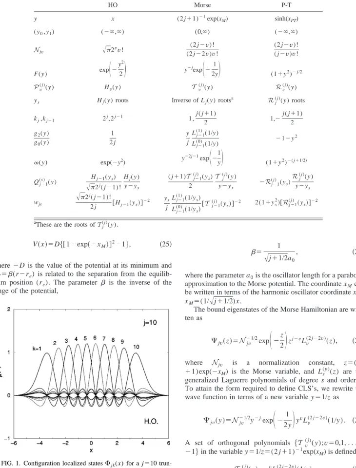
Hv共x兲; v⫽0, . . . , j⫺1, 共24兲where Hv(x) are the Hermite polynomials. This set of j wave functions has the form required to apply the described pro-cedure to form the CLS’s. This case is particularly simple since y⫽x. In Table I the relevant information to build the CLS’s for the truncated harmonic oscillator is shown under the label HO. In Fig. 1 the CLS states for a truncated har-monic oscillator with j⫽10 are shown. They are distributed symmetrically with respect to the origin and each CLS wave function is concentrated around a point y⫽ys, vanishing for
the rest of the roots of Hj( y ).
For the harmonic oscillator the vibrational matrix ele-ments of the coordinate x and the momentum p calculated by using the corresponding CLS are exact due to the quadrature used. This has been checked by comparing the CLS results with numerical ones obtained by integration with harmonic oscillator wave functions.
B. Morse potential
V共x兲⫽D兵关1⫺exp共⫺xM兲兴2⫺1其, 共25兲
where⫺D is the value of the potential at its minimum and xM⫽(r⫺re) is related to the separation from the
equilib-rium position (re). The parameter  is the inverse of the
range of the potential,
⫽ 1
冑
j⫹1/2a0, 共26兲
where the parameter a0is the oscillator length for a parabolic approximation to the Morse potential. The coordinate xMcan
be written in terms of the harmonic oscillator coordinate x as xM⫽(1/
冑
j⫹1/2)x.The bound eigenstates of the Morse Hamiltonian are writ-ten as
⌿jv共z兲⫽N⫺jv
1/2exp
冉
⫺z 2冊
zj⫺vL v
(2 j⫺2v)共z兲, 共27兲
where Njv is a normalization constant, z⫽(2 j
⫹1)exp(⫺xM) is the Morse variable, and Ls
( p)(z) are the generalized Laguerre polynomials of degree s and order p. To attain the form required to define CLS’s, we rewrite the wave function in terms of a new variable y⫽1/z as
⌿jv共y兲⫽Nj⫺v
1/2y⫺jexp
冉
⫺12y
冊
yvL v
(2 j⫺2v)共1/y兲. 共28兲
A set of orthogonal polynomials 兵T v( j)(y );v⫽0,1, . . . , j ⫺1其in the variable y⫽1/z⫽(2 j⫹1)⫺1exp(xM) is defined as
T v
( j)共
y兲⫽yvLv(2 j⫺2v)共1/y兲. 共29兲
TABLE I. Relevant information to construct CLS’s for harmonic oscillator共HO兲, Morse, and Po¨schl-Teller共P-T兲potentials.
HO Morse P-T
y x (2 j⫹1)⫺1exp(xM) sinh(xPT)
(y0,y1) (⫺⬁,⬁) (0,⬁) (⫺⬁,⬁)
Njv
冑
2vv!(2 j⫺v)! (2 j⫺2v)v!
(2 j⫺v)! ( j⫺v)v!
F(y ) exp
冉
⫺y2
2
冊
y⫺j
exp
冉
⫺12y
冊
(1⫹y2)⫺j/2Pv
( j)
(y ) Hv(y ) T v( j)(y ) Rv( j)(y )
ys Hj(y ) roots Inverse of Lj(y ) rootsa Rj
( j)
(y ) roots
kj,kj⫺1 2
j
,2j⫺1 1,j( j⫹1)
2 1,⫺
j( j⫹1) 2
g2(y ) g0(y )
1 2 j
y j
L(1)j⫺1(1/y )
L(0)j⫺1(1/y ) ⫺1⫺y
2
(y ) exp(⫺y2) y
⫺2j⫺1exp
冉
⫺1y
冊
(1⫹y2)⫺( j⫹1/2)Qj⫺1 (s)
(y ) Hj⫺1(ys)
冑
2j( j⫺1)!Hj(y )
y⫺ys
( j⫹1)T j⫺1 ( j)
(ys)
2
T j
( j)
(y )
y⫺ys ⫺Rj⫺1
( j)
(ys)
Rj
( j)
(y )
y⫺ys
wjs
冑
2j共j⫺1兲!2 j 关Hj⫺1共ys兲兴
⫺2 ys
j
L(1)j⫺1共1/ys兲
Lj⫺1 (0) 共
1/ys兲
关T j⫺1 ( j) 共
ys兲兴⫺2 2共1⫹ys
2兲关
Rj⫺1 ( j) 共
ys兲兴⫺2
aThese are the roots ofT
j
( j)
(y ).
The fact that they are polynomials in y can be seen easily since Lv(2 j⫺2v)(1/y ) is a polynomial of order v in 1/y and multiplying this by yv gives a polynomial of order v in y. The coefficients of this polynomial are those of Lv(2 j⫺2v)(1/y ) but in reversed order 关e.g., the coefficient of the term of order n in T v( j)(y ) is the coefficient of orderv ⫺n in Lv(2 j⫺2v)(y )兴. The properties of polynomialsT v( j)( y ) are discussed in Appendix A. In terms of these polynomials, the Morse wave functions are written as
⌿jv共y兲⫽Nj⫺v
1/2
y⫺jexp
冉
⫺ 1 2 y冊
T v( j)共
y兲, 共30兲
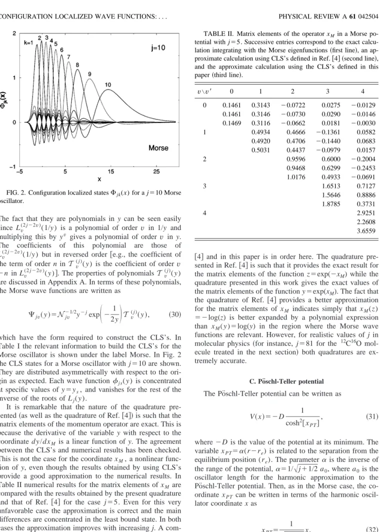
which have the form required to construct the CLS’s. In Table I the relevant information to build the CLS’s for the Morse oscillator is shown under the label Morse. In Fig. 2 the CLS states for a Morse oscillator with j⫽10 are shown. They are distributed asymmetrically with respect to the ori-gin as expected. Each wave function js( y ) is concentrated
at specific values of y⫽ys, and vanishes for the rest of the
inverse of the roots of Lj( y ).
It is remarkable that the nature of the quadrature pre-sented共as well as the quadrature of Ref.关4兴兲is such that the matrix elements of the momentum operator are exact. This is because the derivative of the variable y with respect to the coordinate d y /dxM is a linear function of y. The agreement between the CLS’s and numerical results has been checked. This is not the case for the coordinate xM, a nonlinear
func-tion of y, even though the results obtained by using CLS’s provide a good approximation to the numerical results. In Table II numerical results for the matrix elements of xM are
compared with the results obtained by the present quadrature and that of Ref. 关4兴 for the case j⫽5. Even for this very unfavorable case the approximation is correct and the main differences are concentrated in the least bound state. In both cases the approximation improves with increasing j. A com-ment on the differences between the quadratures used in Ref.
关4兴 and in this paper is in order here. The quadrature pre-sented in Ref. 关4兴is such that it provides the exact result for the matrix elements of the function z⫽exp(⫺xM) while the
quadrature presented in this work gives the exact values of the matrix elements of the function y⫽exp(xM). The fact that
the quadrature of Ref. 关4兴 provides a better approximation for the matrix elements of xM indicates simply that xM(z)
⫽⫺log(z) is better expanded by a polynomial expression than xM( y )⫽log(y) in the region where the Morse wave
functions are relevant. However, for realistic values of j in molecular physics 共for instance, j⫽81 for the 12C16O mol-ecule treated in the next section兲 both quadratures are ex-tremely accurate.
C. Po¨schl-Teller potential
The Po¨schl-Teller potential can be written as
V共x兲⫽⫺D 1
cosh2关xPT兴, 共31兲
where⫺D is the value of the potential at its minimum. The variable xPT⫽␣(r⫺re) is related to the separation from the
equilibrium position (re). The parameter␣ is the inverse of
the range of the potential,␣⫽1/
冑
j⫹1/2 a0, where a0 is the oscillator length for the harmonic approximation to the Po¨schl-Teller potential. Then, as in the Morse case, the co-ordinate xPT can be written in terms of the harmonicoscil-lator coordinate x as
xPT⫽ 1
冑
j⫹1/2x. 共32兲FIG. 2. Configuration localized states⌽jk(x) for a j⫽10 Morse oscillator.
TABLE II. Matrix elements of the operator xM in a Morse po-tential with j⫽5. Successive entries correspond to the exact calcu-lation integrating with the Morse eigenfunctions共first line兲, an ap-proximate calculation using CLS’s defined in Ref.关4兴 共second line兲, and the approximate calculation using the CLS’s defined in this paper共third line兲.
v\v⬘ 0 1 2 3 4
0 0.1461 0.3143 ⫺0.0722 0.0275 ⫺0.0129 0.1461 0.3146 ⫺0.0730 0.0290 ⫺0.0146 0.1469 0.3116 ⫺0.0662 0.0181 ⫺0.0030 1 0.4934 0.4666 ⫺0.1361 0.0582 0.4920 0.4706 ⫺0.1440 0.0683 0.5031 0.4437 ⫺0.0979 0.0157
2 0.9596 0.6000 ⫺0.2004
0.9468 0.6299 ⫺0.2453 1.0176 0.4933 ⫺0.0691
3 1.6513 0.7127
1.5646 0.8886 1.8785 0.3731
4 2.9251
The bound eigenstates of the Po¨schl-Teller Hamiltonian are written as
⌿jv共z兲⫽N⫺jv
1/2P
j
( j⫺v)共z兲, 共33兲
where Njv is a normalization constant, z⫽tanh(xPT), and
Ps( p)( y ) are the associated Legendre functions. These states do not have the form required to define CLS’s关Eq.共1兲兴but it can be achieved by defining a new variable,
y⫽sinh共xPT兲⫽
z
冑
1⫺z2. 共34兲 With this variable a new class of orthogonal polynomialsRv
( j)( y ) can be defined by
P( jj⫺v)共z兲⫽共1⫹y2兲⫺j/2R( j)v 共y兲. 共35兲
In Appendix B it is demonstrated that Rv( j)(y ) are j polyno-mials of orderv(v⫽0,1, . . . , j⫺1) in the variable y that are orthogonal with respect to the weight function (1 ⫹y2)⫺( j⫹1/2). The values ofN
jv and kj are also calculated
there. With these new polynomials the Po¨schl-Teller wave functions can be written as
⌿jv共y兲⫽N⫺jv
1/2共
1⫹y2兲⫺j/2Rv( j)共y兲. 共36兲
These states now have the appropriate form to define the CLS’s. In Table I the relevant information to build the CLS’s for the Po¨schl-Teller oscillator is shown under the label P-T. In this table Pj(y ) are the Legendre polynomials and Pj
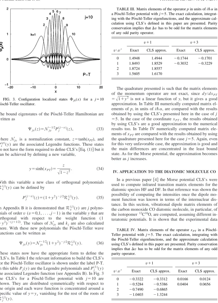
(1) ( y ) the associated Legendre function共see Appendix B兲. In Fig. 3 the CLS’s for a Po¨schl-Teller potential with j⫽10 are shown. They are distributed symmetrically with respect to the origin and each wave function is concentrated around a specific value of y⫽ys vanishing for the rest of the roots of
Rj
( j)(y ).
The quadrature presented is such that the matrix elements of the momentum operator are not exact, since dy /dxPT ⫽
冑
1⫹y2 is not a linear function of y, but it gives a good approximation. In Table III numerically computed matrix el-ements of p, in units of iប␣, are compared with the results obtained by using the CLS’s presented here in the case of j ⫽5. In the case of the coordinate xPT, the results obtained by using CLS’s are a good approximation to the numerical results too. In Table IV numerically computed matrix ele-ments of xPTare compared with the results obtained by usingthe quadrature presented here for the case j⫽5. Again, even for this very unfavorable case, the approximation is good and the main differences are concentrated in the least bound state. As for the Morse potential, the approximation becomes better as j increases.
IV. APPLICATION TO THE DIATOMIC MOLECULE CO
In a previous paper 关4兴 the Morse potential CLS’s were used to compute infrared transition matrix elements for the diatomic species HF and DF. In that reference was shown the possibility of computing the intensities once the dipole mo-ment function was known in terms of the internuclear dis-tance. In this section, vibrational dipole matrix elements of the carbon monoxide CO diatomic molecule, in particular, of the isotopomer 12C16O, are computed, assuming different in-teratomic potentials. It is shown that the experimental data
FIG. 3. Configuration localized states ⌽jk(x) for a j⫽10 Po¨schl-Teller oscillator.
TABLE III. Matrix elements of the operator p in units of iប␣in a Po¨schl-Teller potential with j⫽5. The exact calculation, integrat-ing with the Po¨schl-Teller eigenfunctions, and the approximate cal-culation using CLS’s defined in this paper are presented. Parity conservation implies that⌬v has to be odd for the matrix elements of any odd parity operator.
v\v⬘
v⫹1 v⫹3
Exact CLS approx. Exact CLS approx.
0 1.4948 1.4944 ⫺0.1744 ⫺0.1701 1 1.8493 1.8529 ⫺0.3032 ⫺0.3229 2 1.8724 1.8557
3 1.5605 1.6170
TABLE IV. Matrix elements of the operator xPT in a Po¨schl-Teller potential with j⫽5. The exact calculation, integrating with the Po¨schl-Teller eigenfunctions, and the approximate calculation using CLS’s defined in this paper are presented. Parity conservation implies that⌬v has to be odd for the matrix elements of any odd parity operator.
v\v⬘
v⫹1 v⫹3
Exact CLS approx. Exact CLS approx.
0 ⫺0.3322 ⫺0.3312 0.0166 0.0124 1 ⫺0.5284 ⫺0.5386 0.0404 0.0656 2 ⫺0.7490 ⫺0.6865
are well reproduced by modeling the interatomic interaction with a Morse potential, while major discrepancies are ob-tained by using harmonic oscillator and Po¨schl-Teller poten-tials. This is not surprising, but the main goal is to provide an example of how CLS’s can be a useful tool to study the relevance of different interatomic potentials to describe the anharmonicity in a particular problem.
The CO molecule is of great spectroscopic and astro-physical interest. The rovibrational intensities of this mol-ecule have received considerable attention and much work is devoted to their calculation关9–12兴. In particular, the experi-mental data set used in this section is taken from Ref. 关9兴. The purpose of this work is far from competing with those extensive rovibronic calculations, but, focusing our attention on the purely vibrational problem, we aim to check the CLS’s formalism presented and show its applicability. Within the Born-Oppenheimer approximation the vibrational transition intensities for the electronic ground state band are defined by the matrix elements
R共v→v
⬘兲
⫽具
⌿v兩ˆ兩⌿v⬘典
⫽冕
0
⬁
⌿v*共r兲共r兲⌿v⬘共r兲r2dr,
共37兲
where⌿v(r) are the vibrational wave functions and(r) is the expectation value of the dipole moment for internuclear distance r and electronic ground state functions.
It is assumed, as in Ref. 关4兴, that the vibrational wave functions can be approximated as the eigenfunctions of a 1D potential 共with j bound states兲 and that the dipole moment function is a well behaved function of the internuclear sepa-ration. Using the orthogonality of CLS’s and Eq. 共18兲, Eq. 共37兲can be rewritten as
R共v→v
⬘兲⬇
兺
s⫽1
j
具
j ,v兩CL; j ,s典
共rs兲具CL; j ,s兩j,v⬘典
.共38兲
It is worth noting that the evaluation of this expression is simple, requiring solely the knowledge of the dipole moment function at certain internuclear distances determined by the zeros of the appropriate orthogonal polynomial and the over-lap factors defined in Eq.共15兲.
There are several references that tackle the problem of computing the dipole moment function of the CO molecule, either with a phenomenological approach 关13兴 or as an ab initio calculation 关14,15兴. In the present work an analytical dipole moment function taken from the literature关13兴is em-ployed. With this input the vibrational matrix elements of the dipole moment are computed using the CLS’s formalism for the different potentials presented. The corresponding results for each potential are then compared with the experimental ones.
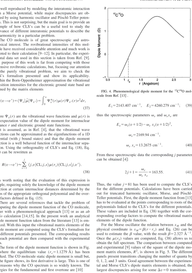
The form of the dipole moment function is shown in Fig. 4, where the equilibrium value (re⫽1.1279 Å) has been marked. The CO molecule static dipole moment is small but, as the figure shows, its first derivative is large. This is one of the reasons why the CO spectrum is so widely known. The energies for the fundamental and first overtone are关10兴
E1⫽2143.407 cm⫺1, E
2⫽4260.279 cm⫺1; 共39兲
thus the spectroscopic parameters eandexeare
Ev⫽e共v⫹1/2兲⫺exe共v⫹1/2兲2,
e⫽2169.94 cm⫺1,
e xe⫽13.2675 cm⫺1. 共40兲
From these spectroscopic data the corresponding j parameter can be obtained 关4兴:
2 j⫹1⫽ e
exe⫽
163.55. 共41兲
Thus, the value j⫽81 has been used to compute the CLS’s for the different potentials. Calculations have been carried out for truncated harmonic oscillator, Morse, and Po¨schl-Teller potentials. First, the dipole moment function from关13兴 has to be evaluated at the points corresponding to roots of the polynomials linked to the CLS’s for the different potentials. These values are included in Eq.共38兲together with the cor-responding overlap factors to compute the vibrational matrix elements of the dipole function.
For the Morse oscillator the relation between xM and the
physical coordinate is xM⫽(r⫺re) and Eq. 共26兲 can be
used to estimate the  value, with the result⫽2.327 Å⫺1. Once the (rk) values are computed, Eq. 共38兲allows us to
obtain the full spectrum. The comparison between computed and experimental关9兴values of the square of the dipole mo-ment matrix elemo-ments, R2, is shown in Fig. 5. The different panels present transitions changing the number of quanta by 0, 1, 2, and 3 units. Good agreement between the experimen-tal and Morse CLS’s dipole matrix elements is obtained, the largest discrepancies arising for some ⌬v⫽0 transitions.
In order to reflect the quality of the results obtained in Fig. 5, Fig. 6 shows the corresponding errors. The quantity plotted isv→v⬘defined as
v→v⬘⫽
Rtheor2 共v→v
⬘
兲⫺Rexpt2 共v→v⬘兲
expt共v→v
⬘兲
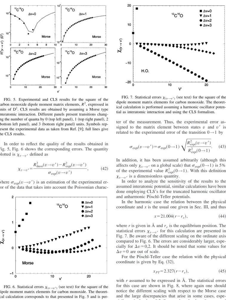
, 共42兲whereexpt(v→v
⬘
) is an estimation of the experimental er-ror of the data that takes into account the Poissoniancharac-ter of the measurement. Thus, the experimental error as-signed to the matrix element between states v and v
⬘
is related to the experimental error of the transition 0→1 byexpt共v→v
⬘
兲⫽expt共0→1兲冑
Rexpt 2 共v→v
⬘兲
Rexpt2 共0→1兲. 共43兲
In addition, it has been assumed arbitrarily 共although this affects onlyv→v⬘on a global scale兲thatexpt(0→1) is 5% of the experimental value Rexpt2 (0→1). With this definition
v→v⬘is a dimensionless quantity.
In order to analyze the sensitivity of the results to the assumed interatomic potential, similar calculations have been done employing CLS’s for the truncated harmonic oscillator and anharmonic Po¨schl-Teller potentials.
In the harmonic case the relation between the physical coordinate and x is the usual one given in Sec. III, and thus
x⫽21.004共r⫺re兲, 共44兲
where r is given in Å and reis the equilibrium position. The
statistical errors v→v⬘ for this calculation are presented in Fig. 7. Be aware of the different scaling on the ordinate axis compared to Fig. 6. The errors are considerably larger, espe-cially for ⌬v⫽0,2. It should be noted that some values for ⌬v⫽0 are out of scale.
For the Po¨schl-Teller case the relation with the physical coordinate is given by Eq.共32兲,
xPT⫽2.327共r⫺re兲, 共45兲
with r assumed to be expressed in Å. The statistical errors for this case are shown in Fig. 8, where again one should notice the different scaling with respect to the Morse case and the large discrepancies that arise in some cases, espe-cially again for⌬v⫽0,2. Some values for⌬v⫽0 are out of scale too.
FIG. 5. Experimental and CLS results for the square of the carbon monoxide dipole moment matrix elements, R2, expressed in units of D2. CLS results are obtained by assuming a Morse type interatomic interaction. Different panels present transitions chang-ing the number of quanta by 0共top left panel兲, 1共top right panel兲, 2
共bottom left panel兲, and 3共bottom right panel兲units. Symbols rep-resent the experimental data as taken from Ref.关9兴; full lines give the CLS results.
FIG. 6. Statistical errors(v→v⬘)共see text兲for the square of the dipole moment matrix elements for carbon monoxide. The theoret-ical calculation corresponds to that presented in Fig. 5 and is per-formed assuming a Morse potential as interatomic interaction and using the CLS approach.
As expected, the best results are obtained for the Morse calculations, as this potential is closer to a realistic molecular interatomic interaction for a diatomic molecule than the other two cases examined. However, this might not be the case when dealing with polyatomic molecules. For instance, it has been suggested that the bending mode in a triatomic molecule is better represented by a Po¨schl-Teller potential 关16兴. The CLS formalism could help in clarifying which kind of anharmonicity is more relevant. It can be concluded that the CLS formalism allows one to obtain analytical formulas that ease the calculations, and it is sufficiently accurate to discriminate between harmonicity and anharmonicity as well as between different types of anharmonicity 共Morse and Po¨schl-Teller兲.
V. SUMMARY AND CONCLUSIONS
In this paper the general formalism for building configu-ration localized states is presented. Their properties are ana-lyzed and analytical expressions for the matrix elements of the operators of interest, including the momentum p and a generic function of the coordinate G(x), are computed.
The CLS states are the eigenfunctions of a certain func-tion of the coordinate in the basis formed by the bound states of the appropriate one-dimensional potential. They provide a simple and numerically appropriate tool to face the problem of molecular vibrations and allow one to reach analytical expressions even for anharmonic wells.
The CLS formalism is worked out for three potentials of interest in molecular physics, providing the necessary ele-ments to build the CLS’s in each case. Finally, we have applied the formalism presented to a real case, the analysis of the 12C16O vibrational intensity spectrum. The results ob-tained through comparison of the calculations carried out with the three examples presented show the sensitivity of the formalism, at the same time reducing the numerical com-plexity of the problem and providing a valuable tool for these problems. In addition, the CLS’s may help in some numerically extensive calculations that make use of a grid of
points where the wave functions are evaluated. In particular, the Morse oscillator CLS’s could provide for these calcula-tions a very interesting alternative to the harmonic approach, as the momentum matrix elements are exact due to the quadrature employed.
ACKNOWLEDGMENTS
This work was supported in part by the Spanish DGICYT under Project No. PB98-1111. We acknowledge useful dis-cussions with F. Iachello, A. Frank, R. Lemus, and V. Szocs. This paper uses data provided by D. Goorvitch in Ref.关9兴as distributed by the Astronomical Data Center at NASA God-dard Space Flight Center.
APPENDIX A
In this appendix we show that the polynomials T v( j)( y ) introduced in Eq.共29兲are in fact orthogonal polynomials and their standardization and differential relations are deduced. The starting point is Eq. 共30兲for the Morse eigenfunctions with the redefined variable y⫽exp(xM)/(2j⫹1), bounded
be-tween zero and infinity, and the polynomials
T v
( j)共
y兲⫽yvLv(2 j⫺2v)共1/y兲. 共A1兲
It is worth noting that the polynomials T v( j)(y ) have the same coefficients as the Laguerre Lv(2 j⫺2v)( y ) but in reversed order; thus the independent term in Lv(2 j⫺2v)( y ) corresponds to the power yv inT v( j)( y ). From the orthonormality of the wave function 共30兲 the following orthogonality relation for the T v( j)( y ) polynomials can be derived:
冕
0⬁
d y y⫺2 j⫺1e⫺1/yT v( j)共y兲T v
⬘
( j)
共y兲⫽Njv␦v,v⬘. 共A2兲
Thus theT v( j)( y ) are orthogonal polynomials in the interval 关0,⬁兴 with weight function(y )⫽y⫺2 j⫺1e⫺1/yand normal-izationNjv. The values of kj and kj⫺1 can be derived in a straightforward way from the information on Laguerre poly-nomials 关7兴,
kj⫽1, 共A3兲
kj⫺1⫽ j共j⫹1兲
2 . 共A4兲
The differential relation of the T ( j) polynomials can be shown to be
g2共y兲 d dyT j
( j)共
y兲⫽g1共y兲T j
( j)共
y兲⫹g0共y兲T j⫺1 ( j) 共
y兲, 共A5兲
with
g2共y兲⫽y
兺
i⫽0
j⫺1
共⫺1兲j⫹i⫺1
冉
j⫺1i
冊
j! 共j⫺i兲!yi
⫽共j⫺1兲!yjL(1)j⫺1共1/y兲, 共A6兲
g1共y兲⫽j
兺
i⫽0
j⫺1
共⫺1兲j⫹i⫺1
冉
j⫺1i
冊
j ! 共j⫺i⫺1兲!yi
⫽j j !yj⫺1L
j⫺1
(0) 共1/y兲, 共A7兲
g0共y兲⫽
兺
i⫽0
j⫺1
共⫺1兲j⫹i⫺1
冉
j⫺1i
冊
j ! 共j⫺i⫺1兲!yi
⫽j!yj⫺1L(0)j⫺1共1/y兲. 共A8兲
APPENDIX B
In this appendix it is shown that the functions Rv( j)( y ) introduced in Eq.共35兲are in fact orthogonal polynomials and their standardization and differential relations are deduced. The starting point is Eq. 共35兲,
Rv
( j)共
y兲⫽共1⫹y2兲j/2P( jj⫺v)共z兲. 共B1兲
We use the definition of the associated Legendre function,
Pj( j⫺v)共z兲⫽共⫺1兲j⫺v共1⫺z2兲( j⫺v)/2d
j⫺vP
j共z兲
dzj⫺v , 共B2兲
where Pj(z) is the Legendre polynomial which can be writ-ten as
Pj共z兲⫽
兺
n⫽0 [ j/2]Cn( j)zj⫺2n. 共B3兲
Taking the corresponding derivatives and using the rela-tion between z and y variables z2⫽y2/(1⫹y2), Eq.共B1兲can be rewritten as
Rv
( j)共
y兲⫽共⫺1兲j⫺v
兺
n⫽0 [v/2]
Cn
( j)共j⫺2n兲! 共v⫺2n兲!y
v⫺2n共1⫹y2兲n,
共B4兲
which shows thatRv( j)( y ) is a polynomial of orderv in the variable y. Straightforward computation of the integral of two of these polynomials with weight function ( y )⫽(1 ⫹y2)⫺( j⫹1/2)gives
冕
⫺⬁ ⬁共1⫹y2兲⫺( j⫹1/2)Rv( j)共y兲Rv
⬘
( j)
共y兲d y⫽Njv␦v,v⬘,
共B5兲
where Njv⫽(2 j⫺v)!/( j⫺v)v!. It is worth noting that the
polynomial Rj( j)( y ) is orthogonal to all the others even if it cannot be normalized. The coefficients of yj inR( j)j (y ) and of yj⫺1 in R( j)j⫺1( y ) are easily obtained by using Eq. 共B4兲 and Eq.共B3兲:
kj⫽Pj共1兲⫽1, 共B6兲
kj⫺1⫽⫺Pj
⬘共
1兲⫽⫺j共j⫹1兲
2 . 共B7兲
Direct computation gives the differential relation of theR( j) polynomials,
g2共y兲 d dyRj
( j)共
y兲⫽g1共y兲R( j)j 共y兲⫹g0共y兲R( j)j⫺1共y兲, 共B8兲
with
g2共y兲⫽1⫹y2, 共B9兲
g1共y兲⫽j y , 共B10兲
g0共y兲⫽⫺1. 共B11兲
关1兴H.-L. Dai and R. W. Field, Molecular Dynamics and
Spectros-copy by Stimulated Emission Pumping 共World Scientific, Singapore, 1995兲.
关2兴M.S. Child and R.T. Lawton, Faraday Discuss. Chem. Soc. 71, 273共1981兲.
关3兴M.S. Child and L. Halonen, Adv. Chem. Phys. 57, 1共1984兲.
关4兴M. Carvajal, J.M. Arias, and J. Go´mez-Camacho, Phys. Rev. A 59, 1852共1999兲.
关5兴P.M. Morse, Phys. Rev. 34, 57共1929兲.
关6兴G. Po¨schl and E. Teller, Z. Phys. 83, 143共1933兲.
关7兴Handbook of Mathematical Functions, edited by M. Abramowitz and I. Stegun共Dover, New York, 1972兲.
关8兴M. Carvajal, J.M. Arias, and J. Go´mez-Camacho, Phys. Rev. A 59, 3462共1999兲.
关9兴D. Goorvitch, Astrophys. J., Suppl. Ser. 95, 535共1994兲.
关10兴J.M. Hure´ and E. Roueff, Astron. Astrophys., Suppl. Ser. 117, 561共1996兲.
关11兴J.M. Hure´ and E. Roueff, J. Mol. Spectrosc. 160, 335共1993兲.
关12兴C. Chackerian, Jr., D. Goorvitch, J.M. Hure´, and E. Roueff, J. Mol. Spectrosc. 165, 583共1994兲.
关13兴C. Chackerian, Jr., R. Farrenq, G. Guelachvili, C. Rossetti, and W. Urban, Can. J. Phys. 62, 1579共1984兲.
关14兴Stephen R. Langhoff and Charles W. Bauschlicher Jr., J.
Chem. Phys. 102, 5220共1994兲.
关15兴Hans-Joachim Werner, Mol. Phys. 44, 111共1981兲.
关16兴F. Iachello and R. D. Levine, Algebraic Theory of Molecules