1
Local sources identification of trace metals in urban/industrial mixed land-use areas 1
with daily PM10 limit value exceedances 2
3 4
Ignacio Fernández-Olmo* (1), Carlos Andecochea (1), Sara Ruiz (1), José Antonio 5
Fernández-Ferreras (1,2), Angel Irabien (1) 6
7
(1) Department of Chemical and Biomolecular Engineering, ETSII y T, University of 8
Cantabria, Santander, Spain 9
(2) Consejería de Medio Ambiente, Cantabria Government 10
11
*Corresponding author: 12
Ignacio Fernández-Olmo: Tel.:+34942206745; Fax: +34942201591, e-mail: 13
Carlos Andecochea: Tel.:+34942201579, e-mail: [email protected] 15
Sara Ruiz: Tel.:+34942201579, e-mail: [email protected] 16
José Antonio Fernández-Ferreras: Tel.:+34942206745, e-mail: [email protected] 17
Angel Irabien: Tel.:+34942201597, e-mail: [email protected] 18
19 20 21
*Manuscript-validated
2
Abstract 1
2
This study presents the analysis of the concentration levels, inter-site variation and source 3
identification of trace metals at three urban/industrial mixed land-use sites of the Cantabria 4
region (northern Spain), where local air quality plans were recently approved because the 5
number of exceedances of the daily PM10 limit value according to the Directive 2008/50/EC 6
had been relatively high in the last decade (more than 35 instances per year). PM10 samples 7
were collected for over three years at the Torrelavega (TORR) and Los Corrales (CORR) sites 8
and for over two years at the Camargo (GUAR) site and analysed for the presence of arsenic 9
(As), cadmium (Cd), chromium (Cr), copper (Cu), lead (Pb), nickel (Ni), titanium (Ti), 10
vanadium (V), molybdenum (Mo), manganese (Mn), iron (Fe), antimony (Sb) and zinc (Zn). 11
Analysis of enrichment factors revealed an anthropogenic origin of most of the studied 12
elements; Zn, Cd, Mo, Pb and Cu were the most enriched elements at the three sites, with Fe 13
and V as the least enriched elements. Positive Matrix Factorisation (PMF) and pollutant roses 14
(Cu at TORR, Zn at CORR and Mn at GUAR) were used to identify the local sources of the 15
studied metals. Analysis of PMF results revealed the main sources of trace metals at each site 16
as road traffic at the TORR site, iron foundry and casting industry at the CORR site and a 17
ferro-manganese alloys industry at the GUAR site. Other sources were also identified at these 18
sites, but with much lower contributions, such as minor industrial sources, combustion and 19
traffic mixed with the previous sources. 20
21
Keywords: Trace elements, Source identification, Positive matrix factorization, Inter-site 22 variation 23 24 25 26 27
3
1. INTRODUCTION 1
The levels of PM10 (suspended particulate matter with an aerodynamic diameter of less than 2
10 µm) in some European urban and industrial areas usually exceed the yearly and daily limit 3
values of 40 and 50 g/m3, respectively, set by the European Air Quality Directive 4
2008/50/EC (Querol et al., 2008; Putaud et al, 2010; European Environmental Agency, 2012). 5
Cantabria is a small coastal region located in northern Spain, where the number of 6
exceedances of the daily PM10 limit value in some urban-industrial mixed land-use areas was 7
higher than the maximum number of exceedances allowed by Directive 2008/50/EC (35 8
instances per year). This Directive states that air quality plans should be developed for zones 9
and agglomerations in which the pollutant concentrations in ambient air systematically exceed 10
the air quality target/limit values. These air quality plans must incorporate, at least, 11
information related to the origin of the pollution, including the main emission sources, the 12
total quantity of emissions from point sources, and information on pollution from long-range 13
sources. Table 1 shows the number of exceedances of the daily PM10 limit value at the 14
monitoring stations of Cantabria from 2003 to 2011. According to the exceedances primarily 15
found at the Los Corrales de Buelna, Camargo and Torrelavega (Barreda) sites from 2003 to 16
2008, three local air quality plans were developed in the Cantabria region (Consejería de 17
Medio Ambiente, Ordenación del Territorio y Urbanismo del Gobierno de Cantabria, 2007; 18
2012a;2012b). 19
The measured mass of PM depends on many sources that are not located near the receptor 20
sites, such as secondary inorganic and organic aerosols and other long-range sources 21
(Lewandowska and Falkowska, 2013; Skyllakoul et al., 2014), sea-salt aerosol (Arruti et al., 22
2011a; Lewandowska and Falkowska, 2013) and some crustal sources (Salvador et al., 2013). 23
However, the emission of particles from local sources increases the levels of PM10 and 24
micropollutants, such as trace metals and some organic compounds (Dongarrà et al., 2007); 25
the main local anthropogenic sources can be mobile (from vehicles) or stationary (residential 26
and industrial combustion and other industrial activities). Considering the number of daily 27
PM10 exceedances at the Cantabria sites (Table 1), a high contribution from local sources to 28
the PM10 levels at the sites of Camargo, Torrelavega (Barreda site) and Los Corrales de 29
Buelna may be anticipated, because the number of daily PM10 exceedances at the other sites 30
in the Cantabrian Air Quality Network is relatively low. 31
4 Trace metals are good tracers of local industrial emissions (Moreno et al., 2006); thus, the 1
source apportionment of metals in urban areas that are influenced by local industrial activities 2
can be incorporated into such air quality plans to help reduce the PM10 levels and their 3
associated toxicity. Two main groups of source apportionment techniques are usually reported 4
in the literature (Viana et al., 2008). The first group consists of source-receptor modeling by 5
means of deterministic models. From a mathematical point of view, this approach is highly 6
complex and requires reliable emission datasets from inventories or direct measurements of 7
pollutants to model the dispersion, transformation, transport and deposition of such 8
contaminants (Maes et al., 2009). The second group of models is based on the statistical 9
evaluation of the pollutants measured at receptor sites. Receptor modeling has been widely 10
applied in source apportionment studies in different environmental matrices, such as rainwater 11
(Junto and Paatero, 1994), bulk deposition (Huston et al., 2012; Fernández-Olmo et al., 2014) 12
and PM10 (Polissar et al., 1998; Almeida et al., 2006; Alleman et al., 2010). Some recent 13
reviews in the literature have addressed the use of receptor models with PM data (Reff et al., 14
2007; Viana et al., 2008). Major components, trace metals, and organic compounds are 15
usually considered in these analyses. Chemical Mass Balance (CMB), Principal Component 16
Analysis (PCA) and Positive Matrix Factorisation (PMF) are the most commonly used 17
techniques (Viana et al., 2008). PMF was developed by Paatero and Tapper (1994) as an 18
alternative to other factor analysis techniques. The major improvement of this technique is 19
that it forces all the values in the solution profiles and factor contributions to be non-negative, 20
which is more realistic than their treatment in PCA. PMF was first applied to precipitation 21
data (Junto and Paatero, 1994) and bulk wet deposition samples (Anttila et al., 1995) with the 22
aim of identifying the most important sources of ions and major elements. Later, PMF was 23
extensively applied to PM10 data for the apportionment of metals and major components 24
(Reff et al., 2007; Alleman et al., 2010). 25
Additionally, methods based on the evaluation of monitoring data, for example, correlating 26
meteorological variables, such as wind direction with levels of air pollutants, have also been 27
used (Eilers, 1991; Somerville et al., 1996), sometimes in combination with receptor 28
modelling (Yue et al., 2008; Alleman et al., 2010; Chan et al., 2011). The relationship 29
between the levels of single pollutants and the wind direction is usually reported by means of 30
pollutant concentration roses, which are polar diagrams that depict how air pollution depends 31
on wind direction (Eilers, 1991). If an ambient air quality monitoring station is markedly 32
5 influenced by the source of a measured pollutant, the corresponding pollutant concentration 1
rose will contain a peak towards the local source (Cosemans and Kretzschmar, 2002). In this 2
work, three urban-industrial mixed land-use areas located in the Cantabria region of northern 3
Spain, where local air quality plans have been established due to the number of exceedances 4
of the daily PM10 value, were selected to study the levels of trace metals and local sources. 5
Trace metals are considered good tracers of local sources and have therefore been chosen in 6
this study to assess the contribution of local anthropogenic activities by using one of the most 7
commonly employed receptor modelling techniques, Positive Matrix Factorisation (PMF). 8
9
2. MATERIALS AND METHODS 10
2.1. Study area 11
Three areas of the Cantabria region, a small coastal area located in northern Spain, which 12
have recently had local air quality plans approved due to daily PM10 level exceedances were 13
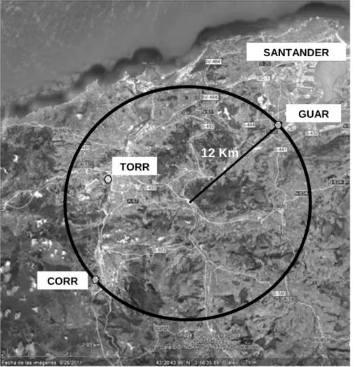
studied in this work: 14
1) In the southern part of Santander Bay, an urban station, Camargo, registered a high number 15
of daily PM10 limit value exceedances (Table 1). PM10 filters were sampled at another 16
station, Guarnizo (GUAR, 43º24'12'' N, 3º50'36'' W, 11 m.a.s.l.), which is located close to the 17
Camargo station (approximately 1 km SW) and may be considered an urban/industrial site. 18
The vicinity of Camargo is an important industrial area for iron, steel and ferromanganese 19
alloys manufacturing. 20
2) An urban/industrial station named CORR (43º15'48'' N, 4º03'51'' W, 89 m.a.s.l.) is located 21
in the town of Los Corrales de Buelna. This site had a high number of daily PM10 22
exceedances, mainly between 2003 and 2007 (Table 1). Industrial activities related to drawing 23
and iron foundry and casting are located in the southern and eastern parts of the town. 24
3) In the town of Torrelavega, a monitoring station named Barreda (TORR, 43º21'43'' N, 25
4º02'47'' W, 13 m.a.s.l.) also registered a high number of daily PM10 exceedances (Table 1). 26
TORR is an urban background site, but is also influenced by traffic and industrial sources. 27
The main industrial activities in this area include pulp and paper, and chemical plants with 28
intensive fossil fuel use. 29
6 As shown in Figure 1, the distance between the monitoring sites is short, and a circle with a 1
radius of 12 km encompasses the three sampling points. 2
3 4
2.2. Sampling and analysis 5
6
PM10 sampling was carried out in 2008 and 2009 at the GUAR site and in 2008, 2009 and 7
2010 at the TORR and CORR sites. Because the PM10 filters were collected within the 8
framework of the three local air quality plans, the sampling was carried out by the local 9
government and the number of filters, the duration of the sampling campaign and the amount 10
of air volume filtered for each sample were fixed by the technical staff of the local 11
environmental authorities. Thus, low volume samplers (2.3 m3/h) were used to collect 48 h 12
samples on quartz micro-fibre filters (47 mm diameter, Sartorius) in 2008 and 2009, and 24 h 13
samples were used in 2010. According to Directive 2004/107/EC, a minimum of 14 % time 14
coverage was used for the studied years. 15
The analysis of arsenic (As), cadmium (Cd), chromium (Cr), copper (Cu), iron (Fe), 16
manganese (Mn), molybdenum (Mo), nickel (Ni), lead (Pb), titanium (Ti), antimony (Sb), 17
vanadium (V) and zinc (Zn) in the PM10 samples was conducted in accordance with the 18
standard UNE-EN 14902:2006 (standard method for the measurements of Pb, Cd, As, and Ni 19
in the PM10 fraction of suspended particulate matter). Each filter was digested using a mix of 20
HNO3 and H2O2 in a microwave digestion system (ETHOS). The digested samples were
21
analysed by inductively coupled plasma mass spectrometry (ICP-MS) on an Agilent 7500 CE 22
with a collision/reaction cell operating in hydrogen mode to avoid matrix interferences. 23
Quality control of the analytical procedure was performed by evaluating the recovery values 24
of the analysed pollutants in a standard reference material (SRM 1649a “urban dust”). The 25
blank contribution from the filters and reagents were evaluated and subtracted from the 26
results. The element recovery obtained from SRM1649a, the average of the filter blanks and 27
the method detection limits (MDLs) are shown in Table 2. Further details about the analytical 28
methodology can be found in Arruti et al. (2010; 2011a). 29
The hourly wind data required to calculate the pollutant and wind roses were available at the 30
CORR and GUAR sites. At the TORR site, the meteorological station was located 1 km SW. 31
The meteorological and major pollutant data were supplied by the Cantabrian Air Quality 32
7 Monitoring Network. The pollutant roses were calculated from the hourly wind direction data 1
and 48 h metal concentration data using the procedure given in Cosemans and Kretzschmar 2
(2002). The computed pollutant concentration rose is a vector with a dimension equal to the 3
number of sectors used, in this case 36. 4 5 (1) 6 where: 7
j: day index for the period under investigation. 8
n: the number of days in the period for which the rose is constructed. 9
i: the wind sector index for the rose. Range of 1-36 for sectors of 10º. 10
ci: the resulting average concentration for wind sector i in all the studied period.
11
pj: the measured concentration on day j.
12
fi,j: the number of hours that the wind came from sector i on day j.
13
αj: a weight function based on the persistence of the wind vector during day j.
14 15
In this case, αj is set to the inverse of the number of wind direction bins on day j with
non-16 zero frequency, nj. 17 18 j 1nj (2) 19 20 2.3. Source apportionment 21
A comprehensive discussion of the theoretical basis of PMF can be found in the literature 22
(Paatero and Tapper, 1994; Reff et al., 2007; Hopke, 2009). Briefly, PMF solves the receptor 23
modelling equation (see equation 3), where the input ambient data matrix (e.g., concentration 24
of metals bound to PM) equals the product of two new matrices, the factor profile (F) and the 25
contribution of each source (G) plus a residual matrix (E). Thus, in matrix form, 26
X = GF + E (3)
27
which can also be written in index notation as 28 ij p k kj ik ij g f e x
1 , where i
1,n;j1,m;k
1,p (4) 29
n j j j i n j j j i j i p f f c , 1 , , 1 , 8 where n is the number of samples and m is the number of species. The coefficients of F and G 1
are calculated for a given number of factors (p). This is an optimisation problem in which the 2
objective function to be minimised is a modified error matrix (Q), which takes into account 3
the uncertainties of each measured pollutant in each sample (ij) with the constraints that each
4
of the coefficients of the G and F matrices is to be non-negative (Hopke, 2000). 5
n i m j ij p k kj ik ij g f x Q 1 1 2 1 (5) 6The global minimum of Q calculated from equation (5) is compared with the minimum value 7
of Q (Qtheoretical) obtained from equation (6):
8
Qtheoretical = nm -(n+m)p (6)
9
The uncertainties of the metal concentrations below the MDL were calculated as 5/6 MDL 10
and as 4xijfor the identified outliers. For data that was greater than the MDL, the 11
uncertainties were calculated according to equation (7): 12
ij = (MDLj2 + (dj xij)2)1/2 (7)
13
which was first used by Anttila et al. (1995) for bulk deposition samples. Equation (7) is also 14
proposed by the EPA PMF 3.0 software (US EPA, 2008), where dj is the error fraction
15
calculated from the geometric average of the relative standard deviation (RSD) for each 16
metal, which is the instrumental error associated with the measurements. Any experimental 17
value below the MDL was replaced by half of the MDL, and the geometric mean was used in 18
place of missing data and identified outliers. 19
With respect to the number of factors, three factors led to the best combination of Q values 20
and significance test results (p-value). A total of 100 random runs were used to ensure that 21
local minima were not obtained. Fpeak=0 was used in the developed models because the
22
rotation of factors from assigning different values of Fpeak did not improve the model
23
performance. 24
The following criteria were considered to select the best models: comparison between the 25
predicted and observed data through the time series, the parity plots, the significance test (p-26
9 value), the difference between the calculated Q and Qtheoretical and the physical meaning of the
1
factor profiles. 2
3
3. RESULTS AND DISCUSSION 4
3.1. Levels of trace elements 5
The mean, standard deviation, maximum, minimum and median values of the concentrations 6
of the studied trace elements are shown in Tables 3, 4 and 5 for the TORR, CORR and GUAR 7
sites, respectively. Some of the studied elements are regulated by the European Air Quality 8
Directives (As, Cd, Ni and Pb) and the annual limit/target values are given for these elements. 9
Additionally, Mn and V are also included in the guidelines of the World Health Organization 10
(WHO). These target/limit/guideline values are summarized in Table 6. 11
Tables 3, 4 and 5 show that the annual mean levels of the metals regulated by the EU (As, Cd, 12
Ni and Pb) do not exceed the EU annual limit/target values (6, 5, 20 and 500 ng/m3, 13
respectively) at any of the sites. However, some individual samples at the CORR site 14
exceeded the annual target value for Ni (i.e., 20 ng/m3): a maximum 48 h value of 52.1 ng/m3 15
was detected in 2008, but the annual mean values (4.5, 3.27, and 3.48 ng/m3 in 2008, 2009 16
and 2010, respectively) were well below the annual target value. The levels of V at the three 17
sites were well below the recommended WHO guideline (1000 ng/m3 on a 24 h basis); 18
however, the annual guideline value for Mn given in the WHO guidelines (150 ng/m3) was 19
exceeded at the GUAR site in 2008. Moreover, maximum 48 h Mn values of 515 and 587 20
ng/m3 were found in 2008 and 2009, respectively. Manganese concentrations may increase to 21
an annual average of 200–300 ng/m3 in the proximity of foundries and to over 500 ng/m3 in 22
the presence of ferromanganese alloys industries (Howe et al., 2004). The GUAR site is 23
located 1 km SW of a plant that produces ferromanganese and silicomanganese alloys. 24
The levels of the studied metals were graphically compared with values that are typically 25
observed at Spanish urban and mixed land-use sites (Querol et al., 2007) in Figure 2. 26
Additionally, Table 7 summarizes the mean metal concentrations detected in different Spanish 27
and European urban and urban/industrial mixed land-use areas. With the exception of Mn, Fe 28
and Zn, the levels of the studied metals at the CORR, TORR and GUAR sites are lower than 29
those observed in other Spanish and European cities. High levels of Mn and Zn were present 30
10 in Llodio (Spain) and Dunkerque (France), which can be explained by the presence of iron 1
and steel industries in these areas (Moreno et al., 2006; Gaudry et al., 2008). Concerning 2
Spanish urban areas, higher concentration levels of Mn and Zn relative to the range detected 3
in Spain can be clearly observed in Figure 2, mainly at the TORR and CORR sites for Zn and 4
the GUAR site for Mn. The levels of the remaining studied elements were within the range, or 5
even below the range, of those found in other Spanish urban areas. 6
At the TORR site, the highest metal concentrations were observed for Zn, Cu, Mn and Cr (see 7
Figure 2a). Although TORR is an urban/traffic mixed site, the level of Cu, a road traffic 8
tracer, is lower than that found at other urban/traffic sites, such as Palermo, Rome and Athens, 9
and industrial sites, such as Llodio, Tarragona and Huelva (see Table 7). The levels of Zn, Cu 10
and Mn were similar in the studied period. However, the Cr level at this site in 2008 was 11
clearly higher than the level in other Spanish cities, whereas its level decreased significantly 12
in 2009 and 2010;. this was attributed to the decrease in coal combustion in the industrial 13
facilities located near the TORR sampling point due to the economic crisis. A strong 14
influence of the economic crisis on the levels of trace metals associated with industrial 15
activities was observed in the first semester of 2009 in the Cantabria region in a previous 16
study (Arruti el al., 2011b). Zinc and Mn had the highest concentration levels at the CORR 17
and GUAR sites. The local industrial activities (iron foundries at CORR and a 18
ferromanganese alloys plant at GUAR) may explain the high values obtained for both 19
elements. This will be discussed further in Source apportionment section. 20
21
3.2. Inter-site variation 22
Considering the relative proximity of the three sampling sites (see Figure 1), an inter-site 23
analysis was performed to determine whether common or local sources affected the levels of 24
trace metals at the studied sites. For this purpose, two techniques were used: the coefficient of 25
divergence (COD) and the inter-site Pearson correlation coefficient for each trace element 26
(Wilson et al., 2005). For these calculations, only samples collected simultaneously were 27
considered. The COD provides information about the degree of uniformity between two 28
sampling sites for a different number of pollutants as seen in equation (8) (Wongphatarakul et 29
al., 1998): 30
11 CODjk= 1/n ((xij-xik)/(xij xik))2 n 1 i
(8) 1where xij represents the average concentration for a trace element i at sites j and k, and n is the
2
number of trace elements. Small inter-site COD values are obtained for sites with common 3
sources, whereas COD values approaching unity indicate great differences (i.e., different local 4
sources at each site). According to previous studies, sites with COD values greater than 0.2 5
are influenced by different types of sources (Wilson et al., 2005). Table 8 shows the inter-site 6
COD values for the studied period, which ranged from 0.22 to 0.37, suggesting that the three 7
sampling sites are influenced by a combination of sources. The smallest COD value was 8
obtained between the CORR and TORR sites (0.22) in 2009; in general, the lowest COD 9
values were calculated for 2009, when the economic crisis was stronger in Cantabria (Arruti 10
et al., 2011b). The decrease in COD in 2009 is attributed to the reduction in local industrial 11
activities while the common sources (mainly road traffic and domestic combustion) were 12
maintained. 13
Additionally, inter-site Pearson correlation coefficients were applied for each studied element, 14
as shown in Table 9. The highest correlations were found for Ti, V and Mo. Titanium is 15
typically found in resuspended urban soil, V is a tracer of combustion, and Mo is good tracer 16
of road traffic (Arruti et al., 2011a). However, Mn, a local industrial marker at the GUAR site 17
due to its proximity to a ferromanganese alloy plant, had low inter-site Pearson correlation 18
coefficients for TORR-GUAR and CORR-GUAR, indicating that the origin of Mn at the 19
CORR and TORR sites is not the ferromanganese alloy plant. 20
The sampling sites were also compared by analysing the enrichment factors of the trace 21
elements (EF). The procedure was based on the standardization of the measured element with 22
respect to a reference element and is shown in equation (9). Reference elements are usually 23
characterized by low occurrence variability, and the most commonly used elements are Al, Ti 24
and Fe. In this study, Ti was selected as a reference because of its relative natural abundance, 25
its even distribution in the crust and the relatively low influence of anthropogenic activities on 26
its observed levels. The reference environmental matrix was the earth's crust and the reference 27
values were obtained from Li et al (2009). 28
EFi = (Xi/Ti)sample/(Xi/Ti)crust (9)
12 In these calculations, Xi,sample and Xi,crust are the concentration in air and the average
1
concentration in the crust of element i. The EF values were calculated for all the studied 2
elements, with the exception of Sb (its crustal concentration was not available), at the three 3
sites and are shown in Figure 3. According to the EF values, the elements can be considered 4
highly enriched (EF>100), intermediately enriched (10<EF<100) and less enriched (EF<10) 5
(Berg et al. 1994). Iron was the least enriched element, followed by V and Mn at the CORR 6
and TORR sites. Although the level of Mn at the three sites was higher than the 7
corresponding range found in the Spanish urban areas (Figure 2), this element is considered 8
highly enriched only at the GUAR site. Figure 3 also shows that the most enriched elements 9
were Zn, Cd, Mo, Pb and Cu at the three sites. Chromium was also highly enriched at the 10
TORR site in 2008, but became intermediately enriched in 2009 and 2010, due to the 11
significant decrease in the concentration in air after 2008. Comparison of the EF values at the 12
three sites indicates that Cu and Mo, which are typically tracers of road traffic, were more 13
enriched at the TORR site, presumably due to the greater impact of road traffic at the TORR 14
site with respect to CORR and GUAR. 15
16
3.3. Source apportionment 17
Three factors were selected to solve the PMF models, which were able to associate more than 18
89% of the metals analysed in the PM10 samples from the three receptor sites. Figures 4, 5 19
and 6 show the source profiles obtained from the PMF analysis of the TORR, CORR and 20
GUAR sites, respectively. Chromium was excluded from the PMF analysis because the MDL 21
was high and the Cr level in many samples was below its MDL. The percentages of each 22
species among the factors are shown by square symbols (right y-axis), and the contribution of 23
each species to the concentration for each factor is given in bar charts (left y-axis). The factors 24
were sorted according to the amount of the metal concentration explained by the model. The 25
contributions of each factor at the three sites are shown in Table 10. 26
At the TORR site, Cu is the main tracer of Factor 1, followed by Fe, Sb and Mo. The 27
contribution of the first factor was approximately 55 %, which is attributed to road traffic. A 28
significant correlation between these four elements and NOx was observed at this site.
29
Although industrial and domestic combustion contribute to total NOx emissions, road traffic is
30
their major source. The highest correlations between NOx and the studied elements were
13 obtained for Fe > Mo > Sb > Cu. Copper and Sb are usually associated with the wear of 1
vehicle brakes (Thorpe and Harrison, 2008). In particular, Cu and Sb were well correlated 2
with organic carbon at the TORR site in a previous work (Moreno, 2010), and the author 3
attributed this to the local traffic around the sampling site. In addition, Mo was well correlated 4
with typical traffic markers, such as NOx and the particle count in a roadside environment
5
(Harrison et al., 2003) and total carbon (Arruti et al., 2011a). The origin of traffic-related Mo 6
has remained unclear in the literature. Molybdenum can be found in engine lubricants as 7
MoS2 (Spada et al., 2012), and incorporated into road dust through oil leakage, but it can also
8
be found in exhaust gases from oil combustion. Sjödin et al. (2010) calculated metal emission 9
factors from road traffic in Sweden and estimated that 24 % of Mo is emitted in exhaust 10
gases, 56 % is due to brake wear and 14 % is due to tyre wear. 11
The second factor is mainly composed of Pb, Cd, As and Zn and is attributed to local 12
industrial activities. In particular, a Zn sulphide ore roasting plant is located 4 km NNE of the 13
sampling site. Zinc had the highest correlation between SO2 and the studied elements. Lead,
14
As, Cd and Fe are the typical impurities found in Zn sulphide ores. Zinc and Fe had the 15
highest mass contribution to factor 2, although both metals were distributed among the three 16
factors. Finally, V and Ni, which are typically associated to combustion of liquid fuels, were 17
the main tracers of the third factor. No significant correlations were observed between Ni and 18
the major pollutants monitored at the TORR site; V was only well correlated with PM10. The 19
influence of the meteorological conditions on the levels of the studied elements was assessed 20
by analysing the wind patterns during the studied period and building and plotting pollutant 21
roses. The wind rose for the TORR site was constructed for the period 2008-2010 and is 22
shown in Figure 7 (a). The prevailing wind direction is WSW, following the direction of the 23
Besaya River towards the sea. A small contribution from the NE sector is also shown in 24
Figure 7(a), corresponding to moderate onshore breezes, mainly present in the summer. 25
Because Cu was the main tracer of the first factor, it was used to compute a pollutant rose 26
calculated from hourly wind direction data and 48 h Cu concentration data using the 27
procedure described in the experimental section. Plotting the pollutant roses on local maps 28
may help to identify the local sources of any metal. Figure 8 shows the Cu rose plotted on the 29
TORR site area. Although the wind rose clearly indicated a prevailing WSW direction, the Cu 30
rose is homogeneously distributed, which agrees with a traffic contribution from all sectors 31
around the sampling site because some motorways and main roads are located nearby. 32
14 Although three local industrial plants are located to the W/SW direction of the sampling site, 1
as shown in Figure 8, the levels of Cu do not appear to be affected by these local plants. 2
At the the CORR site, the first factor explains more than 73 % of the metal contribution, 3
showing high levels of Zn, Mn and Fe. This factor is associated with the local iron foundry 4
and casting plants, which use iron and steel scrap and pig iron as starting materials and some 5
ferromanganese alloys as alloying additions. Steel scrap usually contains high amounts of Zn. 6
The second factor is mainly composed of Pb, Cd, Cu and Sb. The concentration of Zn and Fe 7
in this factor remains noticeable. The composition of this factor is attributed to a mixed 8
contribution from traffic and local industry because Cu and Sb are usually identified as traffic 9
tracers and a local wire drawing plant that contains Zn and Pb baths is located approximately 10
750 m SE of the sampling site (see A3 in Figure 9). Finally, the third factor is associated with 11
V and Ni and is attributed to liquid fuel combustion. At the CORR site, most of the studied 12
elements were well correlated with PM10 and NOx, and only Ni did not have any significant
13
correlation with the major pollutants. 14
The wind rose calculated for the CORR site in 2008-2010 is shown in Figure 7(b). The wind 15
pattern at this site is clearly different than that found at the other sites, with a high 16
contribution from the S, SSE, N and NW sectors. The rose constructed for the main pollutant 17
detected at the CORR site (Zn) is plotted in Figure 9. The main peaks of the rose point to the 18
S, S-SE and E directions, where two iron foundries (A1 and A2) and a wire drawing plant 19
(A3) are located. The highest iron foundry located in the south direction of the sampling site 20
has a capacity of 600 t/year (see A2 in Figure 9). 21
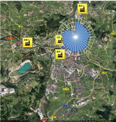
Finally, approximately 40 % of the metal contribution at the GUAR site was associated with 22
the first factor, with a high contribution from Mn and a relevant concentration of Fe. This can 23
be explained by the proximity of a ferro-manganese alloys plant (see A2 in Figure 10). Iron 24
and Mn were well correlated with PM10, SO2, NOx and CO. According to the E-PRTR
25
(Pollutant Release and Transfer Register), these major pollutants are emitted by plant A2 and 26
also by the steel plant located to the N direction (A1 in Figure 10). The profile of the second 27
factor is complex, with intermediate loadings of Cd, Pb, Cu, Ti, Mo, Sb, Fe and Zn. A mixed 28
contribution of traffic and other local industrial sources is assumed. Fe, Zn, Pb and Cd were 29
attributed to the non-integrated steel factory located 4 km to the north of the sampling site 30
(A1), and Cu, Mo and Sb are good tracers of traffic emissions. The highest correlations 31
15 between NOx and the studied elements were obtained for Mo > Cu > Fe. An industrial park
1
located upwind of the receptor point generates substantial traffic from heavy-duty vehicles 2
and may explain the high contribution of this factor (39.8 %). Finally, the last factor is mainly 3
composed of V and Ni and is attributed to liquid fuel combustion. The characteristic wind 4
pattern in the southern portion of Santander Bay is shown in Figure 7(c); the wind rose was 5
calculated at the GUAR site for the period 2008-2009. The predominant wind directions at 6
this site are SW and, to a much lower extent NE, a pattern that has been previously observed 7
(Ruiz et al. 2011): light winds blow predominantly from the SW direction in the fall and 8
winter, whereas moderate onshore breezes from the NE direction are typically observed in the 9
summer. The rose for Mn, the main pollutant at the GUAR site, was plotted on the southern 10
part of the Santander Bay map in Figure 10, together with the rose computed at another site in 11
the bay, Alto Maliaño (ALM). At the ALM site, the Mn peak points to the ferromanganese 12
alloys plant, which agrees with the high contribution of the SW sector observed in Figure 13
7(c). However, at the GUAR site the highest Mn peak also points to the ferroalloy plant, 14
although the contribution of the NE sector is much lower than that of the SW sector as shown 15
in Figure 7(c). This clearly explains the high contribution of the ferromanganese alloy plant to 16
the levels of Mn in the southern portion of the Santander Bay and explains why the highest 17
levels of Mn are observed at the ALM site, as shown in Table 7. 18
19
4. CONCLUSIONS 20
21
A study of the metal levels at three receptor points in the Cantabria region (northern Spain), 22
TORR, CORR and GUAR, where local air quality plans had been developed in response to 23
the number of exceedances of the daily PM10 values in the last decade, was presented. 24
The annual levels of most of the studied elements were lower than those found in other 25
Spanish and European urban/mixed land-use areas. The levels of Zn at the three sites and Mn 26
at the GUAR site were higher than those detected in other urban areas. Such levels of Mn and 27
Zn are only found in urban/industrial mixed land-use areas where iron and steel industries are 28
located. 29
An inter-site analysis among the three sites, which are relatively close to one another, 30
revealed that although road traffic and residential combustion are common sources of metals, 31
local industrial activities increased the inter-site coefficient of divergence (COD) and 32
16 diminished the Pearson inter-site correlation coefficient of the industrial tracers, such as Mn. 1
Moreover, according to the EF analysis, Mn was intermediately enriched at the TORR and 2
CORR sites but highly enriched at the GUAR site, which is located near a ferromanganese 3
plant. The EF analysis also revealed that Fe and V were the least enriched and Zn, Cd, Mo, Pb 4
and Cu were the most enriched elements at the three sites. The models elaborated by the EPA 5
PMF 3.0 software were able to associate more than 89 % of the metals bound to PM10 that 6
were sampled at the studied receptor points. The analysis of the PMF factor profiles, the 7
shapes of the pollutant roses of the main tracers and the previous knowledge of the studied 8
areas were used to identify the main sources of the trace elements at the three sites. At the 9
TORR receptor point, the first factor contributed 55 % of the studied trace element levels, and 10
was mainly attributed to road traffic. The main metal source at the CORR site is an iron 11
foundry and casting industry, with a much higher contribution (73 %) than the other sources. 12
An industrial source (ferromanganese alloys plant) is the most important source at the GUAR 13
site, followed closely by the second factor composed of road traffic and a steel plant. 14
This study demonstrates the important influence of local industrial sources and road traffic on 15
the levels of trace metals at the studied sites. A reduction of particle emissions from these 16
local sources will decrease the levels of such metals and PM10 and therefore help achieve the 17
goals of the EU Air Quality regulation with respect to PM10. 18
19 20 21
17
ACKNOWLEDGEMENTS 1
2
This work was supported by the Spanish Ministry of Science and Innovation (CTM2010-3
16068 and CTM2013-43904R). The authors would also like to thank the Regional 4
Environmental Department of the Cantabria Government and CIMA for providing the PM10 5 samples. 6 7 8 9
18
REFERENCES 1
2
Alleman, L.Y., Lamaison, L., Perdrix, E., Robache, A., Galloo, J.-C., 2010. PM10 metal 3
concentrations and source identification using positive matrix factorization and wind 4
sectoring in a French industrial zone. Atmos. Res. 96, 612–625. 5
6
Almeida, S.M., Pio, C.A., Freitas, M.C, Reis, M.A., Trancoso, M.A., 2006. Approaching 7
PM2.5 and PM2.5-10 source apportionment by mass balance analysis, principal component 8
analysis and particle size distribution. Sci. Total Environ. 368, 663-674. 9
10
Almeida, S.M., Freitas, M.C., Reis, M., Pinheiro, T., Felix, P.M., Pio, C.A., 2013. Fifteen 11
years of nuclear techniques application to suspended particulate matter studies. J. Radioanal. 12
Nucl. Chem. 297, 347–356. 13
14
Anttila, P., Paatero, P., Tapper, U., Jarvinen, O., 1995. Source identification of bulk wet 15
deposition in Finland by positive matrix factorization. Atmos. Environ. 29, 1705-1718. 16
17
Arruti, A., Fernández-Olmo, I., Irabien, A., 2010. Evaluation of the contribution of the local 18
sources on trace metals levels in urban PM2.5 and PM10 in the Cantabria region (Northern 19
Spain). J. Environ. Monit., 12, 1451-1458. 20
21
Arruti, A., Fernández-Olmo, I., Irabien, A., 2011a. Regional evaluation of particulate matter 22
composition in an Atlantic coastal area (Cantabria region, northern Spain): Spatial variations 23
in different urban and rural environments. Atmos. Res. 101, 208-293. 24
25
Arruti, A., Fernández-Olmo, I., Irabien, A., 2011b. Impact of the global economic crisis on 26
metal levels in particulate matter (PM) at an urban area in the Cantabria Region (Northern 27
Spain). Environ. Pollut. 159, 1129-1135. 28
29
Avino, P., Capannesi, G., Rosada, A., 2014. Source identification of inorganic airborne 30
particle fraction (PM10) at ultratrace levels by means of INAA short irradiation. Environ. Sci. 31
Pollut. Res. 21, 4527–4538. 32
33
Berg, T., Royset, O., Steinnes, E., 1994. Trace elements in atmospheric precipitation at 34
Norwegian background stations (1989-1990) measured by ICP-MS. Atmos. Environ. 28, 35
3519-3536. 36
37
Chan, Y.C., Hawas, O., Hawker, D., Vowles, P., Cohen, D.D., Stelcer, E., Simpson, R., 38
Golding, G., Christensen, E., 2011. Using multiple type composition data and wind data in 39
PMF analysis to apportion and locate sources of air pollutants. Atmos. Environ. 45, 439–449. 40
41
CIMA (Centro de Investigación de Medio Ambiente, Gobierno de Cantabria / Environmental 42
Research Center, Cantabria Government), 2010. Evaluación de la calidad del aire y analítica 43
de metales en la fracción PM10 en el Alto Maliaño /Air quality evaluation and metal analysis 44
of the PM10 fraction in Alto Maliaño. Internal Report C-077/2008. 45
46
Consejería de Medio Ambiente, Ordenación del Territorio y Urbanismo del Gobierno de 47
Cantabria (GC), 2007. Plan de Mejora de la Calidad del Aire en el municipio de Los Corrales 48
de Buelna para PM10 / Air Quality Improvement Plan for PM10 in Los Corrales de Buelna. 49
19 1
Consejería de Medio Ambiente, Ordenación del Territorio y Urbanismo del Gobierno de 2
Cantabria (GC), 2012a. Plan de Mejora de la Calidad del Aire para partículas PM10 en 3
Camargo / Air Quality Improvement Plan for PM10 in Camargo. 4
5
Consejería de Medio Ambiente, Ordenación del Territorio y Urbanismo del Gobierno de 6
Cantabria (GC), 2012b. Plan de Mejora de la Calidad del Aire para partículas PM10 en 7
Torrelavega / Air Quality Improvement Plan for PM10 in Torrelavega. 8
9
Cosemans, G., Kretzschmar, J., 2002. Pollution roses for 24h averaged pollutant 10
concentrations by regression, in: Batchvarova, E., Syrakov, D. (Eds.), Eighth International 11
Conference on Harmonisation within Atmospheric Dispersion Modelling for Regulatory 12
Purposes, Sofia, Bulgaria, 14-17 Oct. 2002, pp. 414 - 418. 13
14
Dongarrà, G., Manno, E., Varrica, D., Vultaggio, M., 2007. Mass levels, crustal component 15
and trace elements in PM10 in Palermo, Italy. Atmos. Environ. 41, 7977-7986. 16
17
Eilers, P.H.C., 1991. Penalized regression in action: estimating pollution roses from daily 18
averages. Environmetrics, 2, 25–47. 19
20
European Environmental Agency (EEA), 2012. Air Quality in Europe. 21
22
Fernández-Camacho, R., Rodríguez, S., de la Rosa, J., Sánchez de la Campa, A.M., Alastuey, 23
A., Querol, X., Gonzalez-Castanedo, Y., García-Orellana, I., Nava, S., 2012. Ultrafine particle 24
and fine trace metal (As, Cd, Cu, Pb and Zn) pollution episodes induced by industrial 25
emissions in Huelva, SW Spain. Atmos. Environ. 61, 507-517 26
27
Fernández-Olmo, I., Puente, M., Montecalvo, L., Irabien, A., 2014. Source contribution to the 28
bulk atmospheric deposition of minor and trace elements in a Northern Spanish coastal urban 29
area. Atmos. Res. 145, 80-91. 30
31
Gaudry, A., Moskura, M., Mariet, C., Ayrault, S., Denayer, F., Bernard, N., 2008. Inorganic 32
pollution in PM10 particles collected over three French sites under various influences: rural 33
conditions, traffic and industry. Water Air Soil Pollut. 193, 91-106. 34
35
Harrison, R.M., Tilling, R., Callén, M.S., Harrad, S., Jarvis, K., 2003. A study of trace metals 36
and polycyclic aromatic hydrocarbons in the roadside environment. Atmos. Environ. 37, 37
2391-2402. 38
39
Hopke, P.K., 2009. Theory and application of atmospheric source apportionment. 40
Developments in Environmental Science, 9, 1-33. 41
42
Hopke, P.K., 2000. A guide to positive matrix factorization, 16pp. 43
http://www.epa.gov/ttnamti1/files/ambient/pm25/workshop/laymen.pdf. 44
45
Howe, P.D., Malcolm, H.M., Dobson, S., 2004. Manganese and its compounds: 46
environmental aspects. Concise International Chemical Assessment Document 63. World 47
Health Organization, Geneva. 48
20 Huston, R., Chan, Y.C., Chapman, H., Gardner, T., Shaw, G., 2012. Source apportionment of 1
heavy metals and ionic contaminants in rainwater tanks in a subtropical urban area in 2
Australia. Water Res. 46, 1121-1132. 3
4
Juntto, S., Paatero, P., 1994. Analysis of daily precipitation by positive matrix factorisation. 5
Environmetrics, 5, 127-144. 6
7
Lewandowska, A.U., Falkowska, L.M., 2013. High concentration episodes of PM10 in the air 8
over the urbanized coastal zone of the Baltic Sea (Gdynia-Poland). Atmos. Res. 120, 55-67. 9
10
Li, C., Kang, S., Zhang, Q., 2009. Elemental composition of Tibetan Plateau top soils and its 11
effect on evaluating atmospheric pollution transport. Environ. Pollut. 157, 2261-2265. 12
13
López, J.M., Callén, M.S., Murillo, R., García, T., Navarro, M.V., de la Cruz, M.T., Mastral, 14
A.M., 2005. Levels of selected metals in ambient air PM10 in an urban site of Zaragoza 15
(Spain). Environ. Res. 99, 58–67. 16
17
Maes, J., Vliegen, J., Van de Vel, K., Janssen, S., Deutsch, F., De Ridder, K., Mensink, C., 18
2009. Spatial surrogates for the disaggregation of CORINAIR emission inventories. Atmos. 19
Environ. 43, 1246-1254. 20
21
Manalis, N., Grivas, G., Protonotarios, V., Moutsatsou, A., Samara, C., Chaloulakou, A., 22
2005. Toxic metal content of particulate matter (PM10), within the Greater Area of Athens. 23
Chemosphere, 60, 557-566. 24
25
Moreno, T., Querol, X., Alastuey, A., Viana, M., Salvador, P., Sanchez de la Campa, A., 26
Artiñano, B., de la Rosa, J., Gibbons, W., 2006. Variation in atmospheric PM trace metal 27
content in Spanish towns: Illustrating the chemical complexity of the inorganic urban aerosol 28
cocktail. Atmos. Environ. 40, 6791-6803. 29
30
Moreno, T., 2010. Determinación de fuentes de emisión de material particulado atmosférico 31
en Barreda (Torrelavega) / Determination of emission sources of particulate matter in Barreda 32
(Torrelavega). IDAEA, Technical Report. 33
34
Moreno, T., Pandolfi, M., Querol, X., Lavín, J., Alastuey, A., Viana, M., Gibbons, W., 2011. 35
Manganese in the urban atmosphere: identifying anomalous concentrations and sources. 36
Environ. Sci. Pollut. Res. 18, 173-183. 37
38
Paatero, P., Tapper, U., 1994. Positive matrix factorization: a non-negative factor model with 39
optimal utilization of error estimates of data values. Environmetrics, 5, 111-126. 40
41
Polissar, A.V., Hopke, P.K., Paatero, P., Malm, W.C., Sisler, J.F., 1998. Atmospheric Aerosol 42
over Alaska 2. Elemental Composition and Sources. J. Geophys. Res. 103, 19045-19057. 43
44
Qin, Y., Oduyemi, K., 2003. Chemical composition of atmospheric aerosol in Dundee, UK. 45
Atmos. Environ. 37, 93-104. 46
47
Querol, X., Viana, M., Alastuey, A., Amato, F., Moreno, T., Castillo, S., Pey, J., Rosa, J., 48
Sanchez de la Campa, A., Artíñano, B., Salvador, P., García Dos Santos, S., Fernández-49
21 Patier, R., Moreno-Grau, S., Negral, L., Minguillón, M.C., Monfort, Gil, J.I., Inza, A., 1
Ortega, L.A., Santamaría, J.M., Zabalza, J., 2007. Source origin of trace elements in PM from 2
regional background, urban and industrial sites of Spain. Atmos. Environ. 41, 7219-7231 3
4
Querol, X., Alastuey, A., Moreno, T., Viana, M., Castillo, S., Pey, J., Rodríguez, S., Artiñano, 5
B., Salvador, P., Sánchez, M., 2008. Spatial and temporal variations in airborne particulate 6
matter (PM10 and PM2.5) across Spain 1999-2005. Atmos. Environ. 42, 3964-3979. 7
8
Putaud, J.P., Van Dingenen, R., Alastuey, A., Bauer, H., Birmili, W., Cyrys, J., Flentje, H., 9
Fuzzi, S., Gehrig, R., Hansson, H.C., 2010. A European aerosol phenomenology-3: physical 10
and chemical characteristics of particulate matter from 60 rural, urban, and kerbside sites 11
across Europe. Atmos. Environ. 44, 1308–1320. 12
13
Reff, A., Eberly, S.I., Bhave, P.V., 2007. Receptor modeling of ambient particulate matter 14
data using positive matrix factorization: review of existing methods. J. Air Waste Manage. 15
Assoc. 57, 146–154. 16
17
Ruiz, S., Arruti, A., Fernández-Olmo, I., Irabien, J.A., 2011. Contribution of point sources to 18
trace metal levels in urban areas surrounded by industrial activities in the Cantabria Region 19
(Northern Spain). Proc. Environ. Sci. 4, 76-86. 20
21
Salvador, P., Artíñano, B., Molero, F., Viana, M., Pey, J., Alastuey, A., Querol, X., 2013. 22
African dust contribution to ambient aerosol levels across central Spain: characterization of 23
long-range transport episodes of desert dust. Atmos. Res. 127, 117-129. 24
25
Sjödin, A., Ferm, M., Björk, A., Rahmberg, M., Gudmundsson, A., Swietlicki, E., Johansson, 26
C., Gustafsson, M., Blomquist, G., 2010. Wear particles from road traffic - a field, laboratory 27
and modelling study. Final report. IVL, Swedish Environmental Research Institute. 28
29
Skyllakou, K., Murphy, B.N., Megaritis, A.G., Fountoukis, C., Pandis, S.N., 2014. 30
Contributions of local and regional sources to fine PM in the megacity of Paris. Atmos. 31
Chem. Phys. 14, 2343-2352. 32
33
Somerville, M.C., Mukerjee, S., Fox, D.L., 1996. Estimating the wind directions of maximum 34
air pollutant concentration. Environmetrics, 7, 231-243. 35
36
Spada, N., Bozlakera, A., Chellama, S., 2012. Multi-elemental characterization of tunnel and 37
road dusts in Houston, Texas using dynamic reaction cell-quadrupole-inductively coupled 38
plasma–mass spectrometry: Evidence for the release of platinum group and anthropogenic 39
metals from motor vehicles. Anal. Chim. Acta, 735, 1-8. 40
41
Thorpe, A., Harrison, R.M., 2008. Sources and properties of non-exhaust particulate matter 42
from road traffic: A review. Sci. Total Environ. 400, 270-282. 43
44
US EPA, 2008. EPA Positive Matrix Factorisation (PMF) 3.0 Fundamentals and User Guide. 45
US EPA Office of Research and Development. 46
47
Viana, M., Kuhlbusch, T.A.J., Querol, X., Alastuey, A., Harrison, R.M., Hopke, P.K., 48
Winiwarter, W., Vallius, M., Szidat, S., Prévôt, A.S.H., Hueglin, C., Bloemen, H., Wåhlin, P., 49
22 Vecchi, R., Miranda, A.I., Kasper-Giebl, A., Maenhaut, W., Hitzenberger, R., 2008. Source 1
apportionment of particulate matter in Europe: a review of methods and results. J. Aerosol 2
Sci. 39, 827-849. 3
4
Wilson, J.G., Kingham, S., Pearce, J., Sturman, A.P., 2005. A review of intraurban variations 5
in particulate air pollution: implications for epidemiological research. Atmos. Environ. 39, 6
6444-6462. 7
8
Wongphatarakul, V., Friedlander, S.K., Pinto, J.P., 1998. A comparative study of PM2.5 9
ambient aerosol chemical databases. Environ. Sci. Technol. 32, 3926-3934. 10
11
Yue, W., Stölzel, M., Cyrys, J., Pitz, M., Heinrich, J., Kreyling, W.G., Wichmann, H.E., 12
Peters, A., Wang, S., Hopke, P.K., 2008. Source apportionment of ambient fine particle size 13
distribution using positive matrix factorization in Erfurt, Germany. Sci. Total Environ. 39, 14
133-144. 15
16 17
23 LIST OF TABLES
1 2 3
Table 1. Number of exceedances of the daily PM10 limit value at the Cantabrian Air Quality 4
Monitoring Network stations 5
6
Table 2. Element recoveries obtained from SRM1649a, the average of filter blanks and the 7
method detection limits 8
9
Table 3. Mean (M), standard deviation (s), minimum (Min), maximum (Max) and median (m) 10
of trace metal levels at the TORR site (ng/m3) 11
12
Table 4. Mean (M), standard deviation (s), minimum (Min), maximum (Max) and median (m) 13
of trace metal levels at the CORR site (ng/m3) 14
15
Table 5. Mean (M), standard deviation (s), minimum (Min), maximum (Max) and median (m) 16
of trace metal levels at the GUAR site (ng/m3) 17
18
Table 6. Target/limit/guideline values of metals (ng/m3) 19
20
Table 7. Summary of the mean metal concentrations (ng/m3) detected in different Spanish, 21
European and non-European cities 22
23
Table 8. Coefficient of Divergence (COD) between the TORR, GUAR and CORR sites 24
25
Table 9. Inter-site Pearson correlation coefficients for the studied elements between the 26
TORR, GUAR and CORR sites 27
28
Table 10. Contribution of each factor at the studied sites 29
24 Table 1. Number of exceedances of the daily PM10 limit value at the Cantabrian Air Quality Monitoring Network stations
Year
2003(b) 2004(b) 2005(b) 2006(b) 2007(b) 2008(b) 2009(b) 2010(b) 2011(b) Daily limit value (g/m3) 60 50(a)
55 50(a) 50 50 50 50 50 50 50
Station
Minas 8 18 16 24 38 28 13 11 10 1 10
Zapatón 20 39 29 45 28 16 7 5 3 1 6
Barreda 63 117 63 92 61 92 73 39 36 11 19
Los Corrales de Buelna 61 92 58 75 44 58 45 20 9 11 17
Santander Centro 28 52 24 39 33 28 43 17 13 4 15 Santander Tetuán 31 58 24 37 23 9 27 21 12 1 8 Guarnizo 60 90 52 65 48 29 31 11 8 14 9 Camargo 82 128 88 111 59 61 66 46 25 38 28 Castro Urdiales 49 77 35 50 39 17 7 2 5 16 4 Los Tojos - - - - - - - - - 2 2 Reinosa 28 52 16 22 29 8 6 2 0 6 1
Maximum number of exceedances: 35
(a) Margin of tolerance excluded (b) Natural events not excluded
25 Table 2. Element recoveries obtained from SRM1649a, the average of filter blanks and the
method detection limits
Element Recovery (%) Filter blanks (ng/m3) Detection limit (ng/m3) As 91a 0.05b 0.03b Cd 112a 0.02b 0.01b Ni 115a 1.6b 0.9b Pb 99a 0.5b 0.5b Cu 111a 1.3b 1.1b Cr 68a 1.8b 2.3b Ti n.a 0.6b 1.2b Mn 96 a 1.2b 1.1b V 88a 0.03b 0.05b Mo n.a 0.3b 0.2b Sb 77 0.16 0.02 Fe 75 17.7 4.4 Zn 72 36.6 5.7 a Arruti et al., 2010 bArruti et al., 2011a
26 Table 3. Mean (M), standard deviation (s), minimum (Min), maximum (Max) and median (m) of trace metal levels at the TORR site (ng/m3)
2008 (N=29) 2009 (N=26) 2010 (N=52)
M s Min Max m M s Min Max m M s Min Max m
As 0.18 0.15 <LD 0.72 0.16 0.28 0.2 0.04 0.71 0.23 0.55 0.75 0.03 4.13 0.33 Cd 0.16 0.19 <LD 0.74 0.09 0.16 0.17 0.03 0.83 0.1 0.25 0.52 <LD 3 0.14 Ni 2.81 2.5 <LD 10.4 1.65 4.02 4 0.7 19.4 3.04 3.38 3.7 0.46 19.3 2.11 Pb 12.5 10.7 2.04 44.1 9.1 8.51 7.31 0.91 25.4 4.37 9.24 7.33 0.8 31.8 8.15 Cu 19.3 10.5 <LD 44.8 17.7 18.8 11.4 3.03 56.9 16.7 20.2 11.9 2.92 62.4 17.4 Cr 22.7 58.8 <LD 285 3.45 3.44 3.06 <LD 13.8 1.63 4.86 2 1.83 9.9 4.43 Ti 5.4 8.07 <LD 41.8 3.37 5.38 3.68 0.92 12.9 3.54 6.03 3.97 <LD 19.5 4.91 Mn 22.1 18.4 <LD 76.5 19.7 12.9 9.43 1.87 31.7 10.3 17.5 18.8 1.42 126 12.7 V 1.99 1.41 0.25 5.96 1.69 2.45 1.59 0.32 7.46 2.01 1.75 1.36 <LD 7 1.47 Mo 1.21 0.75 <LD 3.87 0.97 1.35 0.85 0.36 3.27 1.01 1.12 0.79 <LD 3.85 0.89 Sba 1.44 0.66 0.44 2.82 1.36 1.99 1.06 0.27 4.71 2.09 Fea 544 300 113 1,189 514 629 383 79.6 1,770 538 Zna 211 246 <LD 1154 132 354 920 <LD 6326 97.3 a Not measured in 2008 LD Limit of detection
27 Table 4. Mean (M), standard deviation (s), minimum (Min), maximum (Max) and median (m) of trace metal levels at the CORR site (ng/m3)
2008 (N=29) 2009 (N=26) 2010 (N=52)
M s Min Max m M s Min Max m M s Min Max m
As 0.4 0.43 <LD 2.08 0.29 0.32 0.25 0.08 1.14 0.25 0.4 0.36 <LD 2.43 0.34 Cd 0.26 0.54 <LD 2.75 0.08 0.14 0.1 0.01 0.41 0.11 0.13 0.11 <LD 0.66 0.11 Ni 4.5 9.35 <LD 52.1 2.07 3.27 3.51 0.93 18.8 2.27 3.48 3.25 0.68 20.3 2.48 Pb 18.8 21.5 3.25 112 11.8 12.3 11.4 1.7 45.4 7.3 12.1 13.3 0.92 92.5 9.21 Cu 7.32 6.87 <LD 28.5 4.98 6.52 4.99 1.75 23.4 4.8 7.66 5.54 1.37 32 6.31 Cr 7.38 8.8 <LD 34.8 2.87 <LD 1.18 <LD 5.03 <LD 4.87 3.25 1.63 19.4 4.09 Ti 8.1 11.1 <LD 46.9 5.7 5.82 2.52 1.14 10.4 5.64 6.04 4.52 0.84 31 5.23 Mn 32.1 28.8 <LD 134 25 20 14.5 2.64 50.6 14.6 22.3 17.8 <LD 91 17.1 V 1.53 1.51 <LD 6.28 1.07 2.1 1.34 0.47 5.45 1.73 1.35 0.84 0.19 3.33 1.16 Mo 0.82 0.86 <LD 3.41 0.51 0.88 0.8 <LD 3.26 0.54 0.43 0.36 0.06 1.45 0.38 Sba 0.5 0.36 0.05 1.84 0.41 0.63 0.42 0.09 2.26 0.52 Fea 540 439 <LD 1,452 393 562 462 5.66 2,275 476 Zna 188 159 8.38 574 112 219 183 <LD 915 188 a Not measured in 2008 LD Limit of detection
28 Table 5. Mean (M), standard deviation (s), minimum (Min), maximum (Max) and median (m)
of trace metal levels at the GUAR site (ng/m3)
2008 (N=28) 2009 (N=28)
M s Min Max m M s Min Max m
As 0.09 0.12 <LD 0.49 0.04 0.22 0.17 0.04 0.73 0.17 Cd 0.12 0.13 <LD 0.51 0.08 0.24 0.26 0.02 0.97 0.13 Ni 4.24 3.32 <LD 14.6 3.38 4.39 4.75 0.87 21.1 2.72 Pb 12.1 11.1 1.73 57.4 8.59 8.99 8.9 0.55 37.3 6.72 Cu 7.38 6.17 <LD 28.8 5.44 11.4 11 0.86 48.3 8.07 Cr 8.97 5.36 <LD 22.4 7.87 3.75 3.5 <LD 13.9 <LD Ti 5.18 3.9 <LD 23.3 4.78 4.91 3.36 0.6 13.6 4.05 Mn 160 159 6.51 515 82 118 169 1.98 587 35.6 V 2.16 1.62 0.2 7.21 1.66 2.39 1.59 0.46 5.83 2.16 Mo 0.37 0.28 <LD 1.01 0.24 0.66 0.69 <LD 2.83 0.42 Sba 0.82 0.71 <LD 2.37 0.58 Fea 426 344 <LD 1,436 353 Zna 85.4 104 9.73 531 60.1 a Not measured in 2008 LD Limit of detection
29 Table 6. Target/limit/guideline values of metals (ng/m3)
Element EU target/limit value WHO guideline value Averaging time As Cd Pb Mn Ni V 6 5 500 - 20 - - 5 500 150 - 1000 Annual Annual Annual Annual Annual 24 hours
30 Table 7. Summary of the mean metal concentrations (ng/m3) detected in different Spanish and European urban and urban/industrial areas
Type As Cd Ni Pb Cu Cr Ti Mn V Mo Sb Fe Zn
CANTABRIA
Los Corrales de Buelnaa U/I 0.38 0.17 3.7 14 7.29 5.08 6.55 25.2 1.58 0.65 0.59 574 226 Barredaa T/I 1.11 0.2 3.37 10 19.6 9.48 5.7 17.6 1.98 1.2 1.81 601 306 Guarnizoa I 0.16 0.18 4.32 10.5 9.38 6.91 5.05 139 2.28 0.51 0.82 426 85.4 Alto Maliañob I 0.63 0.81 5.01 28.6 10 3.09 - 1,071 1.85 1.2 1.34 477 341 Santanderc U 0.4 0.3 1.2 6.5 4.8 5 2.5 41.1 1.2 0.4 - - - Torrelavegad U/I 0.6 0.3 1.5 19.9 46.9 3.8 15.8 28.7 2.6 3.2 2.7 400 148 SPAIN Llodioe I 1.8 1.2 33 102 32.6 24.6 24.2 86.5 8.3 15.5 3.6 - 417 Tarragonae U/I 0.8 0.3 4.2 25.5 32.9 2.9 22.5 9.2 7.7 2.2 6.9 - 35 Zaragozaf U - - 0.8 18.7 22.8 7.7 - 24.7 6.6 - - 666 212 Huelvag I 6.2 0.7 3.7 14.4 45.3 2.3 46.5 9.6 5.3 12.2 1.6 600 47.4 Spanish rangeh U 0.3-1.6 0.1-0.7 2-7 7-57 7-88 2-8 18-83 4-23 2-15 2-5 1-11 - 14-140 EUROPE Palermo (Italy)i T 1.4 - 8 17 83 9.3 - 18 22 7 19 827 60 Dunkerque (France)j I 2.49 1.27 9.43 34 15.6 4.99 17 99 16 2.14 2.15 1,752 131 Athens (Greece)k I 6.1 3.7 15.9 71.1 43.2 14.5 - 21.1 8.6 - - - - Lisbon (Portugal)l U 0.47 - 4.2 14.6 11.1 - 29.5 6.5 11.2 - 2.6 400 36 Dundee (UK)m U - - 25 21 24 - - - 28 Rome (Italy)n U 2.28 - - - 85.3 - 177 57.1 27.7 - 7.01 - -
U: urban; I: industrial; T: traffic
aPresent study; bCIMA (2010); cArruti et al. (2011a); dMoreno et al (2011); eMoreno et al. (2006); fLópez et al. (2005); gFernández-Camacho et al. (2012); hQuerol et al. (2007); iDongarrà et al. (2007); jGaudry et al. (2008); kManalis et al. (2005); lAlmeida et al. (2013); mQin and Oduyemi (2003); nAvino et al. (2014)
31 Table 8. Coefficient of Divergence (COD) between the TORR, GUAR and CORR sites
2008 2009 2010
CODCORR-TORR 0.30 0.22 0.26
CODCORR-GUAR 0.35 0.27 -
32 Table 9. Inter-site Pearson correlation coefficients for the studied elements between the
TORR, GUAR and CORR sites
CORR-TORR TORR-GUAR CORR-GUAR
As 0.60 0.64 0.40 Cd 0.45 0.59 0.17 Ni -0.18 -0.02 -0.26 Pb 0.64 0.01 -0.08 Cu 0.49 -0.10 0.43 Cr 0.004 0.37 0.08 Ti 0.73 0.68 0.81 Mn 0.73 0.24 0.12 V 0.69 0.84 0.73 Mo 0.79 0.52 0.73 Sb 0.23 0.05 0.79 Fe 0.52 0.24 0.10 Zn 0.55 0.79 0.43
33 Table 10. Contribution of each factor at the studied sites
Site Factor 1 (%) Factor 2 (%) Factor 3 (%)
TORR CORR GUAR 55.3 73.0 40.1 25.2 16.5 39.8 19.5 10.5 20.1