Accepted Manuscript
Title: Thermal characterization of building assemblies by
means of transient data assimilation
Authors: G.M. Soret, D. L´azaro, J. Carrascal, D. Alvear, M.
Aitchison, J.L. Torero
PII:
S0378-7788(17)30967-2
DOI:
http://dx.doi.org/10.1016/j.enbuild.2017.08.073
Reference:
ENB 7902
To appear in:
ENB
Received date:
23-3-2017
Revised date:
22-8-2017
Accepted date:
24-8-2017
Please cite this article as: G.M.Soret, D.L´azaro, J.Carrascal, D.Alvear, M.Aitchison,
J.L.Torero, Thermal characterization of building assemblies by means of transient data
assimilation, Energy and Buildingshttp://dx.doi.org/10.1016/j.enbuild.2017.08.073
This is a PDF file of an unedited manuscript that has been accepted for publication.
As a service to our customers we are providing this early version of the manuscript.
The manuscript will undergo copyediting, typesetting, and review of the resulting proof
before it is published in its final form. Please note that during the production process
errors may be discovered which could affect the content, and all legal disclaimers that
apply to the journal pertain.
1
Thermal characterization of building assemblies by means of transient data assimilation
G.M. Soret1*, D. Lázaro2, J. Carrascal1, D. Alvear2, M. Aitchison3, J. L. Torero1
1 School of Civil Engineering, Building 49 Advanced Engineering Building, Staff House Road, The University of Queensland, St Lucia
QLD 4072 Australia.
2 GIDAI, The University of Cantabria, Avda. Los Castros, s/n, 39005 Santander Spain
3 Faculty of Architecture, Design and Planning, Wilkinson Building, The University of Sydney, NSW 2008 Australia.
Abstract
The quantification of the overall “R-value” of building components is commonly achieved by using numerical models which are generally validated using the standardized Hot Box test. This test set-up follows a complex methodology specifically designed to deliver only the R-value. Modern building assemblies are of a level of complexity that many times a single parameter is insufficient to improve the design of the assembly. This paper proposes a simple thermal test set-up to analyze both transient and steady state heat flow processes, allowing for effective numerical fitting of parameters that describe all internal heat flow processes. As a result, the contribution of each element of an assembly can be evaluated on its overall insulating capabilities, thereby allowing for a truly optimized design solution. Two wall systems including significant thermal bridges have been chosen to illustrate this methodology. The proposed method, not only delivers a steady state thermal assessment as reliable as the standardised Hot Box procedure, but also allows a precise quantification of internal heat flows and the capability to conduct realistic transient state thermal assessments.
Keywords: Thermal bridges; Guarded Hot Box; Small scale thermal test; Numerical modelling.
2
1. INTRODUCTIONThermal resistance value characterizes the thermal insulation properties of building envelope assemblies. R-Value is a prescriptive design parameter included in building codes in Australia and America [1, 2]. In Europe, building codes use thermal transmittance “U-values” instead, this is the inverse of the R-value [3, 4]. Both parameters quantify the insulating properties of the components of a building envelope under steady thermal conditions (Steady State). For a homogenous building component, the R-value defined by Eq. (1) is derived by solving the steady state, one-dimensional, conservation of energy equation [5]. Independent of the boundary conditions, the solution is a linear function where the slope defines the “R” (or “U”) value (Fig. 1).
𝑅𝑇= (𝑘𝐿+ℎ1
𝑇,𝑖+
1
ℎ𝑇,0) (1)
As indicated in the nomenclature section, “L” is the overall thickness of the sample, “k” the global thermal conductivity and “hT” a total heat transfer coefficient that incorporates radiation and convection. The sub-index
“i” denotes internal and the sub-index “o” external to the building.
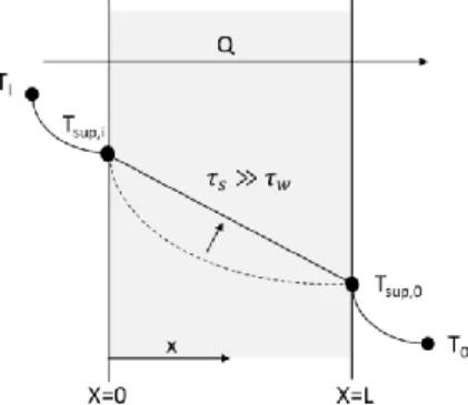
Fig. 1. Steady thermal state representation for a building assembly. A linear temperature distribution through a wall system represents the approximate result from long-term exposure to a temperature difference between the interior and exterior of the assembly. The dotted line represents a more realistic temperature distribution influenced not only by the external temperature variation but also by the material thermal inertia.
The main reason why a steady state model is used by the building industry to describe insulating capacity is because the characteristic time of a particular building assembly to reach steady conditions is generally much shorter than the period of cyclic external temperature variations (𝜏𝑆≫ 𝜏𝑊). Thermal steady conditions can only
be achieved if the assembly reaches steady state faster than the period of cyclic external temperature variations. In this sense, the characteristic time taken by a building assembly to achieve a linear temperature distribution depends on its geometry and the properties, the construction materials and the duration of the major thermal cycles. Eq. (2) presents a scaling analysis of the one-dimensional heat transfer equation using a characteristic
3
time of the cyclic external temperature variation (S) that can then be used to determine the condition needed for
a steady state approach (Eq. (3)), 𝜏𝑤= 𝐿2𝜌𝑐𝑝 𝑘 (2) 𝜕2𝑇̅ 𝜕𝑥̅2= 𝜏𝑤 𝑆 𝜕𝑇̅ 𝜕𝑡̅ 0, 𝑖. 𝑒. 𝜏𝑊 ≪ 𝜏𝑆 (3)
When the period of the temperature cycle 𝑆 is much larger than the characteristic time of the system 𝜏𝑤 then the
resulting temperature distribution is linear. This is the case when building systems thermal performance are considered to be exposed to a seasonal cyclic temperature variation defined by monthly mean values and when daily temperature variations are not significant. Under these circumstances, the thermal assessment deviation by considering pure steady conditions is low and building component insulating properties can be appropriately characterised by means of R-values. It has been noted that under these circumstances, this simplified formulation allows a conservative approach to the design of heating systems in cold climates [6, 7].
The overall R-value of building assemblies can be experimentally obtained by the standardized Hot Box experimental procedure [8, 9, 10, 11]. To date, the research community has improved the Hot Box apparatus mainly by optimising its performance and functionality [12, 13, 14]. Nevertheless, the Hot Box experimental approach remains the same, where only external data to the building system sampled is measured allowing for the calculation of the overall thermal resistance. An inherent limitation of the Hot Box procedure is that the evaluation of the thermal resistance is done after steady state has been attained. This does not allow establishing the importance of transient heat transfer effects nor to provide a comprehensive evaluation of heat fluxes when (𝜏𝑆≤ 𝜏𝑊). These assessments could be of significant values for climates where daily cycles are as important as
seasonal cycles [15].
Building assemblies often include highly thermally conductive structural elements that challenge the concept that thermal resistance can be represented by a single global R-value. This is the well-known “thermal bridge” effect that effectively reduces the R-value with respect to the ideal homogeneous system and creates a three-dimensional heat flow process. Accordingly, building designers have to rely on more detailed calculation procedures to quantify the overall R-value of building design alternatives that include the effect of thermal bridges. In this regard, standardized analytical calculation methods [16] include important simplifications that represent a significant limitation for the evaluation of the thermal performance of unlimited, or at least multiple,
4
design solutions [17]. This is particularly the case when thermal optimization needs to be incorporated as part of an overall optimization process that includes other indicators such as acoustic, structural or fire performance.
An advantage of simplified numerical calculation methods is that they can allow for the resolution of the thermal bridge three-dimensional heat flow problem, provide quantitative information, and accommodate an unlimited number of assembly design variations. Thus, numerical methods are recognized by building designers as effective assessment tools to evaluate building design alternatives [18]. Indeed, specifications to perform numerical models are standardized [19, 20, 21] enabling the definition of design geometries, design material properties and boundary conditions. In this sense, the practice of comparing particular building system R-values calculated by numerical methods with measured data from the Hot Box test has shown that numerical calculation of thermal bridges is straight forward if certain levels of overestimation due to the idealized model geometry are acceptable [22]. Nevertheless, while numerical models can reproduce transient and three-dimensional heat flow features, none of these features can be validated against the steady and one-three-dimensional Hot Box data.
Currently there is no standardized procedure for delivering detailed data on the thermal performance of building assemblies under transient thermal and three-dimensional conditions [23, 24]. Therefore, the validation of existing numerical models is not complete. A number of experimental procedures have been developed by adapting the standardized Hot Box experimental device [8]. Brown and Stephenson developed experimental procedures adapting the standardized Hot Box facility so that programmed constant, ramp or sinusoidal temperatures could be applied on building assemblies [23, 25]. More recent studies have followed similar testing approaches to analyse the influence of structural elements acting as thermal bridges including transient effects [24, 26]. In these tests measurements were performed only at both sides of a building assembly. Given that the Hot Box was never intended to provide this level of detail, these experiments, while useful, are inevitably limited. There is therefore a need to develop a testing procedure that provides validation data that includes transient and three-dimensional effects.
In addition, there is no available experimental procedure that allows the measurement and control of the heating boundary condition so that this could be varied in a systematic way to provide sufficient volume of data for the statistical analysis of the thermal characteristics of construction systems. Given that the Hot Box relies on the
5
variation of the temperature of the airflow, changing the heating condition is extremely cumbersome [23, 24, 25, 26]. Also, the heat flux through the assembly is a function of its thermal properties. Thus, heat-fluxes are very difficult to control and as a result the error between measured and calculated transient response characteristics of a building assembly can be significant, especially when thermal inertia is high [24, 26]. Similar conclusions can be found on literature regarding the standardized fire testing furnace [27].
If the objective is to optimize the design of the assembly to attain particular insulating capabilities, then the Hot Box experimental assessment approach is too coarse. The data available from the Hot Box is measured externally to the building system, does not allow defining details such as internal heat transfer paths, material imperfections, or contact resistances, and does not provide sufficient resolution to deliver three dimensional and transient assessments of construction systems. It is therefore not ideal to perform a realistic evaluation of the contribution of each component to the overall R-value. Finally, the Hot Box does not provide the capacity to vary the heat-flux in a systematic manner, a variation that is necessary for statistical validation of numerical codes.
To address these issues, this study proposes a thermal assessment procedure by means of experimental data from a simpler and more accessible thermal testing set-up that allows for temporal and spatial resolution. This method can be applied to any building envelope system geometry. Through this procedure, heat-fluxes are systematically imposed by using a radiant panel and external and internal information from the building system sampled is measured. This is a small scale thermal testing approach that provides sufficient information for data assimilation processes that can be used to populate a numerical model, allowing for an optimized thermal assessment. Traditional R-values will be used to validate the methodology against collected and existing data.
The paper is organized as follows. In section 2, the details of the proposed methodology are given. In section 3, the application of the methodology to two different systems with the same radiant panel is described, while section 4 presents the validation of the methodology versus an overall R-value measured for a system in the standardized Hot Box. In section 5, a sensitivity analysis of a certain system by applying the model defined with the methodology is included. Finally, section 6 presents the conclusions.
6
2. Materials and MethodsThe methodology proposed in this paper can be applied to any building envelope component allowing for realistic and optimised thermal assessments. Two conventional wall systems containing all relevant construction elements were built; a particular light steel frame (LSF) and a load-bearing structural insulated panel (lbSIP), details of both are presented in the case studies section (i.e. section 3). The wall assemblies studied are used for illustrating the description of the proposed method and to present two case studies applying the methodology. Overall dimensions of the building system sampled are not constrained by the testing procedure or methodology. The wall systems fabrication followed the standard manufacture practices performed by manufacturer and installer in the building industry. Moreover, a third system was used to validate the calculation of the R-Value by the proposed model. This is a different LSF system whose overall R-value was obtained from Hot Box measurements
The thermal performance assessment procedure consists of a thermal testing set-up combined with a thermal computer model of the building system sampled. The thermal test defined is simple and affordable, so that the testing procedure can be readily followed and by which a building system is monitored internally and externally. An accessible heat source is used to apply a heat load on one surface of the building system in a systematic way from ambient temperature until steady heat flow conditions within the system are attained. To illustrate the method proposed, this study uses a stainless steel 5 kW electric radiant heater with a rectangular shape and two bulbs (Infratech WD 5024 Series) that can be seen in Fig. 2a. To quantify the heat loads provided by this particular heater, a heat flux meter was used (SBG01 Hukseflux). Thermal gradients across each layer of a system are measured by a number of thermocouples located at different depths. In this study Type “T” thermocouples were used for both building systems used to illustrate the proposed method (i.e. LSF and lbSIP). Due to the poor thermal insulation of the wiring of this particular type of thermocouples, they were inserted from the unexposed surface of the building systems to avoid possible deviations in temperature measurements caused by heating the thermocouple wire (Fig. 2b). The data acquisition is done using an Agilent 34980A Multifunction data logger. Recorded measurements are compared with a computer model representing the testing approach, so that by following an inverse method best fitting numerical parameters can be obtained. As a result, a model representing realistic internal heat flow processes is obtained. The systematic variation of the
7
heating load allows obtaining sufficient data to deliver statistically valid data assimilation. The model can be finally used for the calculation of the overall R-value of the system under assessment.
2.1 The Small Scale Thermal Testing approach (SSTT)
The SSTT uses the materials and methods described in point 2. Fig. 2a shows the setup used when testing one of the wall assemblies studied (lbSIP). A steady incident heat flux is supplied onto one surface of the wall sampled at ambient conditions, until thermal steady conditions are reached within the sample cross section. This is defined when the temperature measured by all the thermocouples remains steady (Fig. 2c). The test duration is constrained by the moment those circumstances are achieved. Under steady thermal conditions the temperature gradient through the system is linear, so it was decided to locate at least two thermocouples per material layer to define the particular temperature distribution for each material layer. The thermal bridges create a three-dimensional heat transfer process within the system, where the net heat flowing and thus thermal gradients vary over the system depending on the proximity to the more conductive elements. To account for the effect of thermal bridges on the system, thermal gradients need to be measured in each layer in regions closer to and further from the thermal bridge elements. Thus, at least two aligned successions of thermocouples need to be located in the building system. Both of them have to be equidistant from the center of the radiant heat supplied by the electric heater, so that thermocouples placed at the exposed surface can receive the same heat load.
A numerical model of the test is developed to calculate the temperature distribution (Fig. 2d). By assimilating the data into the model, the temperature distributions measured can be compared with a series of numerical temperature distributions until the model input parameters can be obtained. Ultimately, these are the apparent thermal properties of each material component whose values include the effect of contact resistances and potential construction imperfections. Constants linked to the boundary conditions can also be fitted.
8
Fig. 2. View of the small scale experiment approach - lbSIP system case. a) Test set-up b) Thermocouples located in-depth from the unexposed surface c) Temperature history record d) Modelling the test to follow an inverse method.
2.1.1 Definition of the heat source and quantification of the heat flux over the exposed surface of the
system.
When a heat load is applied to a surface of a non-homogeneous building system, it appears as a three-dimensional internal heat flow process that is highlighted when the heat load increases. According to this, a particular heat load can be used to extract the desired apparent thermal properties that can be validated by applying different heat loads. This is achieved by exposing a surface of the assembly to a variety of radiant heat fluxes provided by a radiant panel. The heat flux can be modified by changing the distance (L) between the radiant panel and the exposed surface of the assembly.
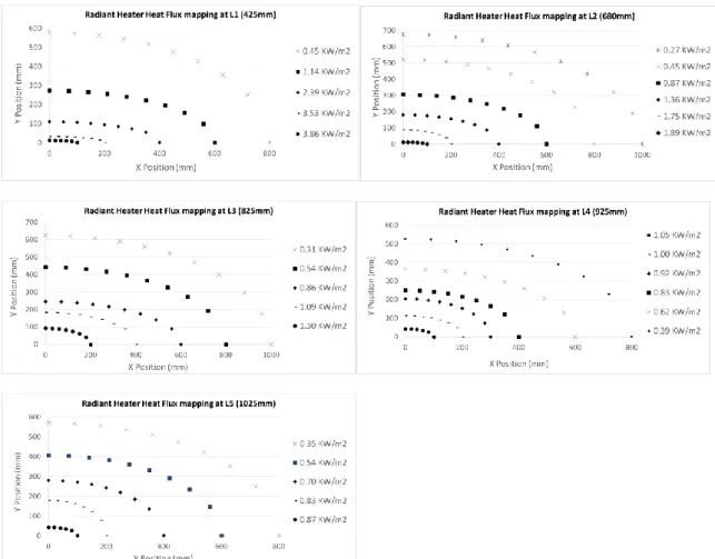
To quantify the heat flux that the building system under study is receiving, a two-dimensional heat flux load produced by the radiant panel has to be mapped at different distances (Fig. 3). The heat flux meter used in this study measured the heat intensities at different points of a two-dimensional grid representing the exposed surface of the building system. Since the heater used in this study is symmetrical with respect to its geometrical centre, it was sufficient to perform the mapping of only one quarter of the system surface. Five two-dimensional heat flux mappings were performed at 425 mm of separation (L1), 680 mm (L2), 825 mm (L3), 925 mm (L4) and 1025 mm (L5). An elliptical heat flux distribution was a good approximation of the heat-flux provided by
9
this particular heater (Fig. 4). By interpolating the heat flux values measured a more detailed heat flux mapping can be obtained to model the heat load applied on the exposed surface of the building system under study.
Fig. 3. Rectangular radiant heater: representation of the two-dimensional geometry and gradient of the radiant heat flux at three different separation distances.
Fig. 4. Heat flux mapping measured at five distances from the rectangular heater used in this study.
2.2 The numerical model
A Finite Element Model (FEM) is developed employing the thermal transient module of ANSYS Workbench V15. As mentioned, the model is firstly used together with the SSTT to define realistic model input data through an inverse procedure. In this case, the model recreates the SSTT approach. Then, the model will be adapted for the overall R-value calculation pursued.
10
2.2.1 FEM calibration from SSTTA three-dimensional geometry of the building system sampled under study is defined with all relevant construction features. Simplifications of potential geometrical complexities in a system are subjected to evaluation from the inverse method procedure.
In order to input the heat flux load on the exposed face of the model, the radiant heat flux mapping geometry obtained is applied to the geometry of the exposed layer for each separation distance. This approach is represented in Fig. (5), where the geometry of the LSF system case study is used to illustrate how the geometry of the exposed layer of a system is adapted according with the geometry of the heat flux mapping obtained. Then, the heat flux values, obtained from the radiant heater mapping, define the constant heat flux applied to each elliptical area of the exposed surface (Fig. 4).
Fig. 5. LSF building system case FEM geometry adapted to model the heat flux load received by the system from the rectangular radiant heater used in this study. .
FEM boundary conditions are obtained from the SSTT approach. The initial model temperature is the ambient temperature measured at the steady state of the SSTT. Similarly, FEM calculation time is set as the experimental time measured to reach steady conditions. A radiant heat losses boundary condition was defined for all external surfaces. According to the ANSYS radiosity solver method only grey diffuse surfaces are considered, so only emissivity values were inputs.
11
This study followed an inverse method to calculate experimentally the apparent thermal conductivity of each component of the system and convective heat losses. As a starting point of the method, a particular convective heat transfer coefficient is set to the model. The building system material properties are obtained from the literature or experimentally, and they are included in the model definition. The FEM outputs are the temperature distributions through the system to be compared with the SSTT temperature distributions measured. Matching calculated and measured temperature distributions deliver the thermal properties of the building system, including apparent thermal conductivities with the effect of construction imperfections and the particular convective heat losses coefficient for the test environment.
2.2.1.1 Equivalent thermal conductivity of air cavities.
In an air cavity, the heat is transferred by radiation and convection processes. Numerically, the air cavity can be represented as an obstruction volume with an equivalent thermal conductivity coefficient that represents a combined effect of the radiation and convection heat transfer processes. This approach can be applied to those building envelope assemblies that include air cavities.
In the literature, there are standards that provide an equivalent thermal resistance for air cavities from where equivalent thermal conductivities can be obtained and used for numerical calculations [28, 29]. As mentioned, none of the internal features of a building system can be validated against the steady and one-dimensional Hot Box data since only external data is measured. Nevertheless, the proposed SSTT allows a direct measurement of the equivalent thermal conductivity for air cavities resulting in realistic data that can be used to populate a numerical model. Thus, the experimental temperature data from three thermocouples (1, 2 and 3) is used, as represented in Fig. 6. Considering that we know the thermal conductivity of Material 2, it is possible to estimate the net heat flowing between points 2 and 3 by applying Eq. (4), where i and j belong to points 2 and 3 respectively. Considering the same net heat flow through the whole system, and the temperatures measured in 1 and 2, the equivalent air thermal conductivity coefficient can be obtained.
𝑞𝑖−𝑗= 𝑘𝑖𝑗
12
Fig.6. Location of thermocouples to estimate the equivalent thermal conductivity of an air gap layer.
2.2.2 The system overall R-value FEM calculation
Once the apparent thermal conductivities are defined, the characteristic heat flow process within the system under analysis is defined and it is followed until thermal steady state is attained. For the overall R-value calculation purpose the edge boundary conditions in the model are assumed to be adiabatic. While the heat transfer within the assembly is three-dimensional, the overall heat transfer remains one-dimensional. The FEM outputs are the surface temperatures and the net heat flowing through the system (expressed per unit area), from where R-values are calculated considering nodal mean values at exposed and unexposed surfaces. The overall surface-to-surface resistance “Rc;op” is characteristic of the system and it is not dependant of the environment and can be calculated using Eq. (5). The air-to-air resistance (R-value) is the Rc;op value adding the surface resistance values at both sides of the system as express Eq. (6).
𝑅𝑐;𝑜𝑝= (𝑇𝑒𝑥𝑡.𝑠𝑢𝑟𝑓.−𝑇𝑖𝑛𝑡.𝑠𝑢𝑟𝑓.) 𝑞 ( 𝑚2𝐾 𝑊 ) (5) 𝑅 − 𝑣𝑎𝑙𝑢𝑒 = 𝑅𝑐;𝑜𝑝+ 𝑅𝑠𝑖+ 𝑅𝑠𝑒 ; 𝑅𝑠𝑖/𝑒=ℎ1 𝑇𝑖/𝑒 (6) 3. Case studies
As mentioned, the methodology proposed in this paper can be applied to any building envelope component to achieve realistic and optimised thermal analysis. As demonstrations, the R-Value assessment was carried out on the Light Steel Frame (LSF) and on the load-bearing Structural Insultaed Panel (lbSIP), both include internal structural elements that thermally bridge the core insulating layer material and construction imperfections. For this, all SSTT are conducted using the same radiant heater and data used to describe the method proposed. Then, this study includes a quantitative comparison of the overall R-value obtained with the ideal R-value of the same system with no thermal bridges.
13
3.1 The LSF wall systemA building company provided a particular LSF wall system assembly from which the geometry has been defined. The overall dimensions of the system sample are 1200 mm in height and 900 mm in width. A cross-section of the system is shown in Fig. 7a, where it can be seen that steel stud voids are filled with 92 mm mineral wool insulation material. The external cladding is formed by 12mm plywood panel and the internal lining is a 12mm plasterboard panel. An 18mm air cavity is created by placing timber battens between the steel frame and the plywood panel. In Fig. 7b the sample is shown without the plasterboard layer to display the steel stud. Due to the characteristic anisometric nature of this LSF building assembly, this study will analyse possible differences in the insulating capabilities of the system by applying the heat flux from both directions.
Fig. 7. LSF system cross-section representation of the sample built to conduct this study. Steel stud placed in the middle of the LSF wall sample.
3.1.1 Small scale experiment set-up and data measured - LSF.
According to the procedure proposed, two successions of thermocouples are placed through the system. Fig. 8 represents the SSTT set-up where it can be seen that the thermocouples are arranged in the sample from the unexposed surface to avoid deviations in temperature measurement caused by heating the thermocouple wire. Fig. 8 shows the representation of thermocouple locations on two cross-section lines through the LSF sample, both located on the metal stud (red points) and following a line assumed to receive the lowest influence of the thermal bridge (blue points). Similar configuration is followed when the plasterboard layer is exposed by inverting the heater and the wiring location.
14
Fig 8. Small scale experiment approach when the external cladding of the system is exposed to a steady heat load.
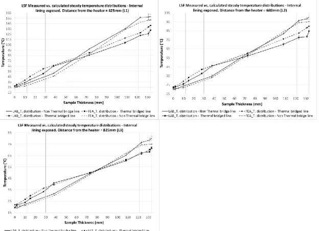
The steady state thermal conditions for this system were achieved in approximately 3 hours. Nevertheless, to ensure steady state conditions, testing time was set to 5 hours after heating of the sample commenced. At this time, the measured temperatures were collected and plotted for both cases when the system is placed at the defined distances L1, L2 and L3 from the electric radiant heater. To quantify the data accuracy a series of three tests were performed for each distance. Fig. 9 shows the representation of the cross-section temperature distribution obtained by the bench scale test when the LSF system wall is exposed to different heat loads at both the external cladding and the internal lining. Error bars indicate the standard error from mean temperatures measured where the maximum value observed for the all tests was 4.7 °C.
Fig. 9. Temperature distribution of the LSF system wall exposed to different heat loads at both the external cladding and internal lining. Grey vertical lines represent layer system interfaces
3.1.2 FEM fitting parameters: comparison of measured and calculated temperature distributions.
As mentioned, the apparent thermal conductivities and the characteristic heat losses of the system can be directly extracted from the SSTT outcome by the inverse process. The characteristic heat losses can be obtained
15
from a single test and extrapolated to the others. For obtaining apparent properties of the LSF system when the external cladding is exposed, a distance L1 was selected, and distances L2 and L3 were used for validation. For the internal lining surface exposed case, distance L3 was used to extract apparent properties and distances L1 and L2 for validation. As starting point, initial FEM material properties input data has been measured by a Hot Disk Thermal Constant Analyser for all the LSF system material components with the exception of the steel frame and the reflective foil, which have been obtained by the inverse process itself. A mean deviation between calculated and measured temperature distributions lower than 10 % appears to be good enough, so it sets the end-point of the inverse process. Air cavity equivalent thermal conductivities calculated and used by the model are included in Table 1, where it can be seen how this value changes depending on the system surface sample. The reason for this could be the fact that different LSF systems were tested for each surface and they could include different assembly faults that generates different internal radiative and convective heat transfer processes. Table 2 includes FEM fitting thermal conductivities of the LSF system for both the external cladding and internal lining surfaces exposed cases.
Table 1
Mean equivalent thermal conductivities values (W/mK) of the air cavity obtained from the SSTT series and the final mean value included in FEM. (*) First SSTT for extracting apparent properties
Mean equivalent Air Cavity thermal conductivities SSTT at 425mm (L1) SSTT at 680mm (L2) SSTT at 825mm (L3) FEM input
Internal lining exposed - Plasterboard 0.087 0.096 *0.068 0.083
External cladding exposed - Plywood *0.016 0.018 0.018 0.017
Table 2
FEM fitting thermal conductivities input values LSF Material
Thermal conductivity (W/mK)
Plywood - External Cladding 0.183
Timber Batten 0.173
Reflective Foil 2.000
Steel Frame 30.000
Mineral Wool 0.033
Plasterboard - Internal Lining 0.234
Matching mean convective heat transfer losses for system surfaces have been obtained for the SSTT for both system exposure cases (Table 3), where its dependency on the system surface temperature can be seen in Eq. (7). A mean radiant heat loss coefficient value over the system surface is calculated from modelled surface temperatures by Eq. (8). The mean total heat losses can be calculated with the Eq. (9). Comparing both hr and hc equations, it can be seen that although both coefficients depend on surface temperature, the radiation dependence is higher (i.e. exponent 4 against 1/3). For this reason, the mean total heat losses variation at the exposed surface when varying the system heat load is mainly affected by heat radiation losses. Constant
16
convection losses can be assumed under the particular testing environment. Table 4 includes ht mean values calculated from the three SSTTs. In Fig. 10 a linear correlation is established between the total heat losses and the heat flux of the tests.
ℎ𝑐 = 0.13𝑘2⁄3(𝜇𝐶η𝑝2𝑔𝛽) 1 3 ⁄ (𝑇𝑠− 𝑇𝑎)1⁄3 (7) ℎ𝑟= 𝜎𝜀(𝑇𝑠 4−𝑇𝑎4) (𝑇𝑠−𝑇𝑎) (8) ℎ𝑡= ℎ𝑐+ ℎ𝑟 (9) Table 3
FEM convection heat transfer loss coefficients (W/m2K) for each SSTT case. (*) First SSTT for extracting heat losses
SSTT at 425mm (L1) SSTT at 680mm (L2) SSTT at 825mm (L3) LSF system exposing
the external cladding
Exposed surface *14.0 14.0 14.0
Not exposed surfaces *25.0 25.0 25.0
LSF system exposing the internal lining
Exposed surface 19.0 18.0 *18.0
Not exposed surfaces 45.0 45.0 *45.0
Table 4
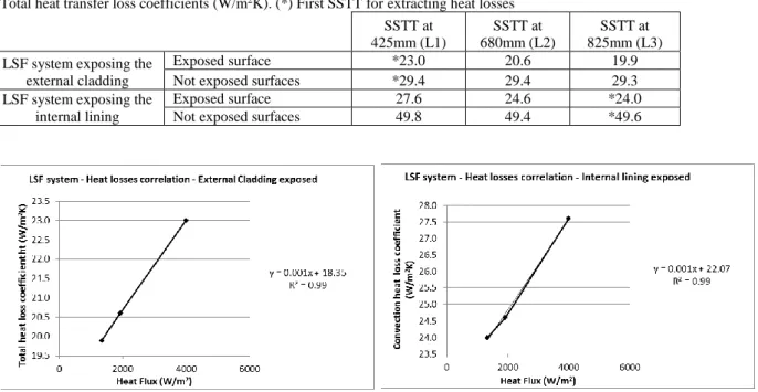
Total heat transfer loss coefficients (W/m2K). (*) First SSTT for extracting heat losses
SSTT at 425mm (L1) SSTT at 680mm (L2) SSTT at 825mm (L3) LSF system exposing the
external cladding
Exposed surface *23.0 20.6 19.9
Not exposed surfaces *29.4 29.4 29.3
LSF system exposing the internal lining
Exposed surface 27.6 24.6 *24.0
Not exposed surfaces 49.8 49.4 *49.6
Fig. 10. Total heat loss coefficients correlation for the exposed surface of both tests cases.
Fig. 11 and Fig. 12 show the corresponding fitting FEM and measured temperature distributions, for both the external cladding and internal lining surfaces exposed cases.
17
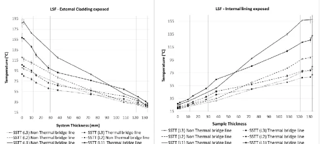
Fig. 11. Comparison of measured and calculated temperature distribution: External cladding exposed. Grey vertical lines represent layer system interfaces
Fig. 12. Comparison of measured and calculated temperature distribution: Internal lining exposed. Grey vertical lines represent layer system interfaces
18
3.1.3 LSF system overall R-value calculation – FEM Thermal Bridge influence quantification.
In order to quantify the overall resistance in both directions of heat influence on the system, the proposed methodology is followed to obtain surface-to-surface Rc;op values (Table 5). In order to obtain the Rc;op values of the equivalent homogeneous system, it has to be changed the steel stud and timber batten thermal properties into the mineral wool and air cavity thermal properties respectively. Analytical calculation of the Rc;op value following the ISO 6946:2007 [16] is included in the Table 5. Calculations are made for three SSTT heat flux cases obtaining the same characteristic Rc;op values as expected.
The effect of the thermal bridge is quantified by comparing numerical calculation for both real life (𝑅𝑐;𝑜𝑝𝑟𝑒𝑎𝑙, which
includes thermal bridge) and equivalent homogeneous cases (𝑅𝑐;𝑜𝑝ℎ𝑜𝑚.) (Table 5). The detrimental effect of thermal
bridge (Def) is calculated by applying Eq. 10.
𝐷𝑒𝑓𝑓 =
𝑅𝑐;𝑜𝑝ℎ𝑜𝑚.−𝑅𝑐;𝑜𝑝𝑟𝑒𝑎𝑙
𝑅𝑐;𝑜𝑝ℎ𝑜𝑚. (10)
In both cases the detrimental effect of the thermal bridge is approximately 70 %. Finally, to calculate air-to-air resistance values, both internal and external surface resistance values have to be defined. From the SSTT the internal surface resistance values are defined as the inverse of the heat losses at the unexposed surface of the system (Eq. (6) and Table 4). The external surface resistance value is obtained from the heat losses at the exposed surface. Table 6 shows these values together with the pursued R-values of the LSF system for both exposure cases.
Table 5
Surface-to-surface resistance values (m2K/W) numerically and analytically calculated.
LSF system - External Cladding exposed
LSF system - Internal Lining Exposed
LSF equivalent Homogeneous system – Analytical Rc;op 4.0 3.1
LSF equivalent Homogeneous system - Numerical Rc;op 4.0 3.1
LSF Real life Numerical Rc;op validated with SST 1.2 1.0
Detrimental effect of thermal bridge 71 % 67 %
Table 6
Air-to-air resistance values (m2K/W).
SSTT Mean value
FEM Rsi 0.03
FEM Rse 0.04
LSF External Cladding R-value (test conditions) 1.2
19
3.2 The lbSIP wall systemAn lbSIP wall system assembly is studied to validate the model. The overall dimensions of the system sample are 800 mm of height and 600 mm of width, and it is geometrically symmetric both vertically and horizontally. A cross-section of the system is shown in Fig. 13a. The panels are comprised of 144mm thick expanded polystyrene foam (EPS) core laminated with 12mm magnesium oxide (MgO) layers that form both the external cladding and the internal lining. It includes an MgO spline mid width (i.e. load bearing element) and edges enclosed with 33mm MgO panels. In Fig. 14b, the lbSIP assembly is shown where some panels have been removed to see better the internal components.
Fig. 13. LbSIP system sampled cross-section representation built to conduct this study.
3.2.1 Small scale experiment set-up and data measured - lbSIP.
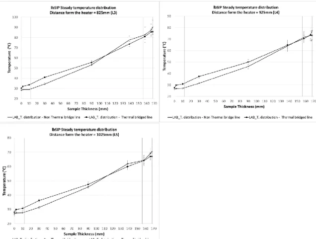
The SSTT set-up follows the procedure described for the previous LSF system. Due to the low softening temperature point of similar EPS products [30, 31, 32] the radiant heater is placed at further distances than in the LSF sample case to avoid material degradation. Thus, the measured temperatures were collected and plotted when the system is placed at the defined distances L3, L4 and L5 from the electric radiant heater. In this case, steady state thermal conditions were observed in a much longer period of time (24 hours). Again, to quantify data accuracy a series of three tests are performed for each distance. Fig. 14 shows the temperature distribution obtained for each separation distance from the heater. Error bars indicate the standard error from mean temperatures measured where the maximum value observed for the all tests was 4.4 °C.
20
Fig. 14. LbSIP system wall temperature distribution obtained. Grey vertical lines represent layer system interfaces.
3.2.2 FEM fitting parameters: comparison of measured and calculated temperature distributions.
Due to the nature of the laboratory where the SSTT series was performed, system surrounding conditions changed in relation to those SSTT performed for the LSF systems, as did matching mean convection heat transfer losses hc (Table 7). Table 8 includes ht mean values calculated from the three SSTT. A linear correlation can be established to predict the system total heat losses under any testing heat load conditions (Fig. 15).
Table 7
FEM convection heat transfer loss coefficients (W/m2K) for each SSTT case. (*)First SSTT for extracting heat losses
SSTT at 825mm (L3) SSTT at 925mm (L4) SSTT at 1025mm (L5)
lbSIP system
Exposed surface 16.0 16.0 *16.0
Not exposed surfaces 29.0 29.0 *29.0
Table 8
FEM Total heat transfer loss coefficients (W/m2K) where implicit hr values are calculated be considering the FEM
temperatures modelled at both exposed and not exposed system surfaces. (*) First SSTT for extracting heat losses
SSTT at 825mm (L3) SSTT at 925mm (L4) SSTT at 1025mm (L5)
LSF system
Exposed surface 35.6 35.2 *35
21
Fig. 15. Total heat loss coefficients correlation.
Like in the LSF testing case, thermal properties of the lbSIP system elements have been measured with the Hot Disk Thermal Constant Analyser. In contrast with the previous case, the simplicity of the lbSIP panel geometry and its precise manufacturing process results in low levels of construction imperfections, allowing a good match with the FEM geometry. Thus, measured and first calculated temperature distributions fit more accurately, resulting in a mean deviation lower than 5% (Fig. 16). So, the material properties measured initially are deemed to be the apparent properties for this case (Table 9).
Table 9
FEM fitting thermal conductivities (W/mK) input values
lbSIP Material Thermal conductivity
MgO 0.357
22
Fig. 16. Comparison of measured and calculated temperature distribution when exposing the lbSIP building system sampled. Grey vertical lines represent layer system interfaces.
3.2.3 LbSIP system overall R-value calculation – FEM Thermal Bridge influence quantification.
Table 10 shows the surface-to-surface Rc;op calculated values for the lbSIP system for both the equivalent homogeneous system and the real system, together with the quantification of the effect of the thermal bridge. The detrimental factor between real and equivalent homogeneous systems is 79 %. Similarly to the LSF system case, the air-to-air R-value is calculated accordingly, resulting in an overall R-value of 1.2 m2K/W.
Table 10
Surface-to-surface resistance values (m2K/W) numerically and analytically calculated.
LSF system - External Cladding exposed
lbSIP equivalent Homogeneous system – Analytical Rc;op 5.6
lbSIP equivalent Homogeneous system - Numerical Rc;op 5.6
lbSIP Real life Numerical Rc;op validated with SSTT 1.2
23
4. Validation of the proposed methodTraditional R-values are used in this study to validate the methodology against collected and existing data. In his thesis, Amundarain built a Guarded Hot Box apparatus [17, 33, 34] to test a particular LSF building design assembly to quantify its air-to-air thermal transmittance U-value (i.e. inverse of the R-value). This study uses the numerical model of the proposed method to calculate the overall R-value of Amundarian LSF system. In this case, no SSTT is conducted to extract numerical fitting parameters, so values from different sources are used instead. Then, both numerically calculated and Amundarin Hot Box R-value are compared.
In order to highlight the simplicity of the proposed SSTT approach a brief description of the Hot Box apparatus built by Amundarian is presented (Fig. 17).
Fig. 17. Guarded Hot Box built by Amundarain.
The standardized Guarded Hot Box test consists of placing a building system sample of a particular area “A” between a hot and cold insulated chamber. The expected measurements are the net heat flowing through the system, and the environmental temperatures at the hot and the cold chamber at steady state conditions. To take into account the Hot Box construction imperfections, a calibration factor “F” is defined by performing
24
preliminary tests with a reference material [35]. Ultimately, data measured is included in Eq. (11) to calculate the overall U-value of the system tested.
U − value = FA(TQnet
em−Tec) (11)
The net heat flowing through the system is obtained by measuring the heat input in the hot side when heat losses are minimized. To achieve this, the hot side is arranged by building a metering Box and a Guarded Box equipped with a temperature thermopile arrangement to minimize system lateral heat losses, together with a digital controller. Additionally, heating elements are included to both compensate heat losses to the hot chamber surroundings and establish the heat input to the system sampled. Furthermore, a number of active components were included in the chambers during the test to control and to measure environmental conditions. The most representatives are; a number of AC/DC fans to control air velocities within metering, guarded and cold chambers, baffle surfaces in the metering and cold chambers to achieve a uniform heat radiation process, thermocouples connected to a data logger to measure temperatures at the system sampled surface, baffle surfaces, and air in the chambers, from where chamber environmental temperatures can be obtained. Once the Hot Box apparatus arrangement is optimised and calibrated, a LSF system sample with a total area of 2.4 x 2.4 m2 was tested (Fig. 18). It was composed of two layers of plasterboard in the unexposed side (12.5 mm each) fixed to a steel stud with a web of 140 mm, filled by mineral wool of 120 mm of thickness and a density of 70 kg/m3 with air cavities at both sides of 10 mm thickness. On the other side of the steel stud there was a second layer of mineral wool of 30 mm thickness and a density of 180 kg/m3. The external surface was made of an aluminium honeycomb panel (20 mm of thickness) to which an adhesive and a render coat were applied. According to Hot Box measurements and Eq. (11) the mean experimental U-value obtained by Amundarain for his particular LSF system was 0.29 W/m2K. The net heat flow achieved by the Hot Box assembly delivers the measured mean surface temperatures at both sides of the system sample that represent the boundary conditions that can be implemented in a numerical model to define the net heat flowing through the modelled system. According to this, in his study Amundarain performed two-dimensional finite difference model calculations to compare both measured and numerically calculated U-values. Using generic material properties from literature, a numerical U-value of 0.26 W/m2K was obtained with a deviation lower than 0.04 W/m2K from the Hot Box measurements, which can be assumed as valid according to similar research studies with LSF assemblies [28].
In this study, the numerical boundary conditions considered are a heat flux load together with radiant and convective heat losses at the surfaces of the system, which define the net heat flowing through the system.
25
Together with either generic material properties or those extracted from the SSTT, mean temperatures at both exposed and unexposed system surfaces can be obtained. Together, these allow for the calculation of the overall U-value of the system including the effect of thermal bridges. In order to compare both numerical boundary conditions approaches, a numerical calculation of the Amundarian LSF system has been performed through the three-dimensional finite element model. To simplify the geometry in the FE model, the red area marked in Fig. 18 has been considered, in which dashed lines define cross-sectional boundaries where a condition of symmetry has been applied, and the continuous line is assigned an adiabatic condition. Fig. 19 shows a cross-section view of Amundarian’s multilayered LSF system developed for the model. The structural elements can be seen passing through the mineral wool insulating layer (yelow coloured lines).
Fig.18. Amundarain’s System Geometry: Front view.
Fig. 19. Amundarain’s System Geometry: Cross-section view.
An equivalent thermal conductivity for the air cavities of 0.05 W/mK is used as the mean value obtained from both LSF SSTT measurements performed in this study. The thermal conductivity coefficients considered in our model are included in Table 11. Three different sources were used in our model [17, 37, 38]. Heat loss values included in the model at both exposed and unexposed sides are those obtained from the LSF system tested when exposed to the external cladding, from which internal and external surface resistances are calculated.
26
Table 11
Amundarain’s System: Thermal conductivities.
Furthermore, a number of simulations were performed with different heat flux loads to compare the effect of the heat flux on the U-value results. Heat fluxes of 800 W/m2, 1200 W/m2 and 1500 W/m2 were chosen as they appeared to create similar net heat flow values to those considered on Amundarain’s Hot Box method. From Table 12 and 13 it can be observed that the mean U-value calculated by the proposed numerical model is very close to that obtained by the standardized Hot Box method. As expected, when including Amundarian’s material thermal properties in the FE model, the numerical U-value calculated result to be very close to that calculated by his FD model. On the other hand, it is seen that material properties from other sources from literature (Toolbox in this case) appear to fit better the Hot Box calculated U-value since deviations are even lower. A SSTT on Amundarian’s LSF system could validate numerical material properties data.
Table 12
U-value obtained by the experimental Hot Box method performed by Amundarain.
Hot Box Net HF input (W/m2) 12.67 15.35 18.43
Calibrated Hot Box U-value (W/m2K) 0.29
Table 13
U-value comparison: Hot Box method and proposed FE model.
Material properties JTonino [37] Amundarain [17] Toolbox [38]
Heat Flux Model (W/m2) 800 1200 1500 800 1200 1500 800 1200 1500
Mean net HF (W/m2) 11.00 16.13 19.79 11.00 15.80 19.42 11.64 17.02 20.86
Equivalent Uc;op FEM (W/m2K) 0.28 0.28 0.28 0.27 0.27 0.27 0.29 0.29 0.29
Equivalent Uvalue FEM (W/m2K) 0.27 0.27 0.27 0.27 0.27 0.27 0.29 0.29 0.29
DIF HOT BOX and FEM Uvalue (W/m2K) 0.02 0.02 0.02 0.03 0.03 0.03 0.01 0.01 0.01
5. Sensitivity analysis of the LSF Building system for a design change strategy.
Since the SSTT delivers experimental information for each material of the building system sampled, a realistic contribution of principal element components to the overall surface-to-surface Rc;op can be established, from which the overall air-to-air overall R-value is obtained according to particular surface resistance values. This way, building designers can rely on realistic analysis for design decision purposes. The LSF system case is used in this study to illustrate this approach.
Material k (W/K.m) [17] k (W/K.m) [37] k (W/K.m) [38]
Plasterboard 0.25 0.179 0.17
Steel Stud 60 54 54
Mineral wool LD 0.031 0.036 0.04
27
The sensitivity analysis consists in varying thermal conductivity values of each component of the LSF system to determine how each component is affecting the Rc;op of the whole system. Then, these alternative Rc;op values are compared with the existing Rc;op taken as base design. Tables 14 and 15 show how the overall Rc;op of both LSF system cases tested varies when changing thermal conductivity values of each component. Indeed the resulting apparent thermal conductivity of the air cavity is lower in the sample tested when the internal lining is exposed, so the sensitivity analysis always delivers higher Rc;op. As expected from this analysis, it can be seen that the material used for structural purposes has the biggest impact on the overall Rc;op with respect to the equivalent homogeneous system, and when selecting a material with 75% lower thermal conductivity, the overall Rc;op of the system improves by 53% closer to the ideal homogeneous system. Alternatively, the next material that could be changed is the material used to create the air cavity (i.e. timber batten) which can improve the overall Rc;op up to 45%.
Table 14
Sensitivity analysis for the LSF System – internal lining exposed case
LSF system layer kbase (W/mK) kbase+75% (W/mK) Overall Rc;op (W/m²K) kbase+75% Comparison with Rc;op Base design (1.2W/m2K) kbase-75% (W/mK) Overall Rc;op (W/m²K) kbase-75% Comparison with Rc;op Base design (1.2W/m2K) External Cladding 0.183 0.320 1.1 -7% 0.046 1.5 25% Timber Batten 0.173 0.304 1.1 -10% 0.043 1.7 45% Steel Frame 30 52.500 1.0 -16% 7.500 1.8 53% Mineral Wool 0.033 0.058 1.0 -12% 0.008 1.3 14% Internal Lining 0.234 0.410 1.1 -6% 0.059 1.4 22% Air cavity 0.017 0.030 1.1 -5% 0.004 1.3 8% Table 15
Sensitivity analysis for the LSF System – external cladding exposed case
LSF system layer kbase (W/mK) kbase+75% (W/mK) Overall Rc;op (W/m²K) kbase+75% Comparison with Rc;op Base design (1.0 m2K/W) kbase-75% (W/mK) Overall Rc;op (W/m²K) kbase-75% Comparison with Rc;op Base design (1.0 m2K/W) External cladding 0.183 0.320 1.0 -7% 0.046 1.3 22% Timber Batten 0.173 0.304 1.0 -9% 0.043 1.3 29% Steel Frame 30 52.500 0.9 -16% 7.500 1.6 53% Mineral Wool 0.033 0.058 0.9 -16% 0.008 1.2 17% Internal Lining 0.234 0.410 1.0 -8% 0.059 1.3 24% Air cavity 0.083 0.146 1.0 -5% 0.021 1.1 5% 6. Conclusions
This study proposes a novel assessment procedure to evaluate building component insulating capabilities under both thermal steady and transient thermal conditions. The assessment method proposed is achieved by means of
28
numerical models complemented by experimental data from a simple thermal testing set-up that allows for temporal and spatial resolution. This is a small scale thermal testing (SSTT) approach that provides by inverse method sufficient information for data assimilation processes that can be used to populate the numerical model. The resulting material properties define internal heat conduction characteristics that account for construction imperfections or contact resistances. Once a realistic model is achieved, it can be adapted to evaluate insulating properties such as the R-value or U-value (both inverse values). This study justifies the use of this insulating parameter for building envelope components located in those geographical locations where daily temperature variations remain low compared to large seasonal temperature variations.
A particular Light Steel Frame assembly (LSF) and a load-bearing Structural Insulated Panel system (lbSIP) have been thermally assessed by calculating the steady state overall R-value to illustrate the proposed method. The detrimental effect of thermal bridges is quantified in both cases and the effect of building construction quality on the overall insulating capabilities is discussed. Through this process the contribution of each layer component, in particular air cavities, is assessed for the LSF system case.
The overall R-value calculated with the proposed method is validated by assessing a third building assembly whose overall R-value was obtained by the standardized Hot Box apparatus. The mean U-value calculated by the model using generic material properties from literature is very close to that obtained by the standardized Hot Box method, reaching a difference of up to 0.01 W/m2K.
Thus, it is demonstrated that a numerical analysis, complemented by a simple and affordable thermal experimental approach, allows for a reliable quantification of the overall R-value of real-life building system samples as it does the standardized Hot Box test. Further, a realistic evaluation of the contribution of each component on the overall R-value is obtained, allowing for an enriched and optimized thermal assessment.
7. Nomenclature
AT Area
hT,i Internal total heat transfer coefficient hT,o External total heat transfer coefficient
29
hT Total heat transfer coefficient
ht Mean total heat losses
hc Mean convective heat transfer coefficient hr Mean radiant heat transfer coefficient
k Global thermal conductivity
L Thickness of a building system
Q Heat flow
Qnet Net heat flowing through a system R-value Thermal resistance
Rc;op Surface-to-surface resistance Rsi Internalsurface resistance Rse Externalsurface resistance RT Total thermal resistance
x Depth of a building system
𝑥̅ Depth over total thickness
T Temperature
𝑇̅ Temperature over the cyclic temperature amplitude
Ti Internal temperature
To External temperature
Tem Environmental temperature in the hot chamber at steady state conditions Tec Environmental temperature in the cold chamber at steady state conditions Tsup,i Internal surface temperature
Tsup,o External surface temperature
t Time
𝑡̅ Time over the cyclic period
ρ Density
cp Specific heat
w Characteristic time for a building system to reach steady state conditions
c Period of a cyclic temperature variation
30
g Gravitational acceleration
Air kinematic viscosity
Air dynamic viscosity
Compressibility for perfect gases
Acknowledgements
This study has been developed thanks to the funding provided by the Australian Research Council, together with the contribution of Happy Haus Pty Ltd, Hutchinson Builders Pty Ltd, Vision Developments Australia Pty Ltd and the Fire laboratory facilities at The School of Civil Engineering of The University of Queensland. The contribution of Mr. Ian Pope and Mr. Andy Wong, from The University of Queensland is also acknowledged. The authors appreciate the invaluable effort done by the partners involved in the study and the Spanish Ministry of Economy and Competitiveness for the PYRODESIGN and EVACTRAIN Project grant, Ref.: BIA2012-37890 and TRA2011-26738 respectively, financed jointly by FEDER funds.
References
[1] National Construction Code 2016 volumes [2] 2015 International Energy Conservation Code
[3] Directive 2010/31/EU of the European Parliament and of the Council
[4] Rockwool International a/s group corporate affairs the way towards nearly zero energy buildings in EU, 2012
[5] T. Bergman, A. Lavine, F. Incropera, and D. DeWitt, "Fundamentals of heat and mass transfer, 2011," USA: John Wiley & Sons. ISBN, vol. 13, pp. 978-0470, 2015.
[6] M. S. Owen and H. E. Kennedy, "ASHRAE handbook: fundamentals," SI edition, ASHRAE, 2009. [7] M. G. Davies, Building heat transfer: John Wiley & Sons, 2004.
[8] BS EN ISO 8990:1996 Thermal insulation –Determination of steady-state thermal transmission properties – Calibrated and guarded hot box
31
[10] R. Robert, P.E Zarr, A History of Testing Heat Insulators at the National Institute of Standards and Technology, Gaithersburg, MD 20899, 2001
[11] Russian GOST 26602.1-99.
[12] C.J. Schumacher, D. Ober, J. Straube, A. Grin, Development of a new Hot Box Apparatus to Measure Building Enclosure Thermal Performance, Proceedings of Buildings XII, 2013 ASHRAE
[13] C. Buratti, E. Belloni, L. Lunghi, M. Barbanera, Thermal Conductivity Measurements By Means of a New ‘Small Hot-Box’ Apparatus: Manufacturing, Calibration and Preliminary Experimental Tests on Different Materials, Int J Thermophys (2016) 37:47
[14] P. Modi, R. Bushehri, C. Georgantopoulou, L. Mavromatidis, Design and development of a mini scale hot box for thermal efficiency evaluation of an insulation building block prototype used in Bahrain, Advances in Building Energy Research, 2016
[15] S. V. Szokolay, Introduction to architectural science : the basis of sustainable design, Third edition. ed. [16] BS EN ISO 6946:2007 Building components and building elements — Thermal resistance and thermal
transmittance — Calculation method
[17] A. Amundarain, Assessment of the Thermal Efficiency, Structure and Fire Resistance of Lightweight Building Systems for Optimised Design, PhD Thesis, the University of Edinburgh, 2007
[18] BRE 443:2006, Conventions for U-value calculations
[19] EN ISO 10211-1:2007, Thermal Bridges in building construction – Heat flows and surface temperatures – Detailed calculations
[20] ISO 10077-2:2012, Thermal performance of windows, doors and shutters – calculation of thermal transmittance. Part 2: Numerical method for frames
[21] BS EN ISO 10456:2007 Building materials and products- hygrothermal properties – tabulated design values and procedures for determining declared and design thermal values
[22] J. Rose, S. Svendsen, Validating Numerical Calculations against Guarded Hot Box Measurements, Nordic Journal of Building Physics Vol.4, 2004.
[23] W. Brown and D. Stephenson, "Guarded hot box procedure for determining the dynamic response of full-scale wall specimens- Part I," in the 1993 Winter Meeting of ASHRAE Transactions. Part 1, 1993, pp. 632-642.
32
[24] K. Martin, A. Campos-Celador, C. Escudero, I. Gómez, and J. Sala, "Analysis of a thermal bridge in a guarded hot box testing facility," Energy and Buildings, vol. 50, pp. 139-149, 2012.
[25] W. Brown and D. Stephenson, "Guarded hot box measurements of the dynamic heat transmission characteristics of seven wall specimens-Part II," ASHRAE Transactions, vol. 99, pp. 643-660, 1993. [26] J. Sala, A. Urresti, K. Martín, I. Flores, and A. Apaolaza, "Static and dynamic thermal characterisation of a
hollow brick wall: Tests and numerical analysis," Energy and Buildings, vol. 40, pp. 1513-1520, 2008. [27] Maluk, C., Bisby, L., Krajcovic, M., & Torero, J. L. (2016). A heat-transfer rate inducing system (H-TRIS)
test method.Fire Safety Journal.
[28] EN ISO 10211-1:2007, Thermal Bridges in building construction – Heat flows and surface temperatures – Detailed calculations
[29] ISO 10077-2:2012, Thermal performance of windows, doors and shutters – calculation of thermal transmittance. Part 2: Numerical method for frames
[30] Knaufinsulation, Safety Data Sheet/Product Information Sheet KI_DP_306-UK, 2011 [31] Styrene Products, Inc. Expanded Polystyrene Material Safety Data Sheet (EPS MSDS)
[32] J. P. Hidalgo-Medina, Performance-Based Methodology for the Fire Safe Design of Insulation Materials in Energy Efficiency Buildings, 2015
[33] BS 874-1:1986. Methods for determining thermal insulating properties. Introduction, definitions, and principles of measurement.
[34] BS 874-3.1:1987. Methods for determining thermal insulating properties with definitions of thermal insulating terms.
[35] BS EN 13163:2001. Thermal insulation products for buildings. Factory made products of expanded polystyrene. Specification.
[36] J. Tonino, Developing a methodology to investigate the thermal performance of prefabricated housing wall panels using finite element analysis, Bachelor of Engineering Thesis, 2014, The University of Queensland
[37] The Engineering ToolBox, [online] Engineeringtoolbox.com. Available at: