Numerical validation of the complex Swift-Hohenberg equation for lasers

Numerical validation of the complex Swift-Hohenberg equation

for lasers

J. Pedrosa , M. Hoyuelos1'2'5 1, and C. Martel3

1 Departamento de Fisica, Facultad de Ciencias Exactas y Naturales, Universidad Nacional de Mar del Plata Mar del Plata, Argentina

2 Consejo Nacional de Investigaciones Cientificas y Tecnicas, CONICET, Argentina

3 Departamento de Fundamentos Matematicos, ETSI Aeronauticos, Universidad Politecnica de Madrid

Abstract. Order parameter equations, such as the complex Swift-Hohenberg (CSH) equation, offer a simplified and universal description that hold close to an instability threshold. The universality of the description refers to the fact that the same kind of instability produces the same order parameter equation. In the case of lasers, the instability usually corresponds to the emitting threshold, and the CSH equation can be obtained from the Maxwell-Bloch (MB) equations for a class C laser with small detuning. In this paper we numerically check the validity of the CSH equation as an approximation of the MB equations, taking into account that its terms are of different asymptotic order, and that, despite of having been systematically overlooked in the literature, this fact is essential in order to correctly capture the weakly nonlinear dynamics of the MB. The approximate distance to threshold range for which the CSH equation holds is also estimated.

PACS. 42.65.Sf Dynamics of nonlinear optical systems; optical instabilities, optical chaos and complexity, and optical spatio-temporal dynamics - 05.45.-a Nonlinear dynamics and chaos

1 Introduction

The complex Swift-Hohenberg (CSH) equation is an or-der p a r a m e t e r equation t h a t provides a reduced descrip-tion of a variety of systems [1], such as Rayleigh-Benard convection [2], optical p a r a m e t r i c oscillators [3-5], Cou-ette flow [6], nematic liquid crystal [7], magnetoconvec-tion [8], p r o p a g a t i n g flame front [9] and photorefractive oscillator [10,11] among others. In t h e case of lasers op-erating near peak gain (small detuning), a derivation of t h e CSH equation for class A and C lasers was obtained in [12,13], s t a r t i n g from t h e semiclassical Maxwell Bloch (MB) equations [14-18], t h a t provide a general descrip-tion of transverse p a t t e r n s in two levels, wide a p e r t u r e and single longitudinal mode lasers. For class B lasers, such as CO2 a n d semiconductor laser, CSH equations have been obtained in [19] and [20] respectively. (For an explanation of t h e classification of lasers, see Ref. [21]). Experimen-tal observations of p a t t e r n s in wide a p e r t u r e lasers were reported in, for example, [22-26] (for reviews on p a t t e r n formation in nonlinear optical systems, see [27-29]).

T h e deduction of a generic order p a r a m e t e r equation greatly simplifies t h e theoretical description of t h e sys-tem. B u t it is i m p o r t a n t t o note t h e limitation of this kind of model equations, as Cross and Hohenberg s t a t e in

their review ([1], p . 874): "it is t r u e t h a t m a n y properties of nonequilibrium systems are encountered in these equa-tions, and indeed m a n y h a r d problems (...) m a y profitably be addressed in t h e simple framework provided by these equations. However, it is only as a p e r t u r b a t i v e expansion valid in a small region near threshold t h a t t h e y provide a quantitative description of real experimental systems, and results m a y be even qualitatively misleading if applied far from threshold".

The argument of a qualitative only scope of the model

equation is usually invoked to justify the application of the

CSH equation far from threshold. The qualitative

correct-ness is difficult to be theoretically established, but, on the

other hand, the capacity to produce quantitative

predic-tions can be determined from the numerical integration of

both, the original system of Maxwell Bloch equations and

the CSH equation. The results of the comparison between

the numerical simulations of the CSH and the MB

equa-tions is what we present in the subsequent secequa-tions of this

paper. We can obtain from the simulations the relative

er-ror that introduces the approximation and estimate how

far from threshold we can increase the pump while

keep-ing a small relative error. Also, this numerical comparison

between the CSH and the MB equations provides a

con-firmation of the main result presented in [31]: that the

CSH equation for the description of the weakly nonlinear

dynamics of the system near threshold (derived in [12,13])

necessarily contains terms of different asymptotic order.

2 The complex Swift-Hohenberg equation

and its numerical phase diagram

The Maxwell-Bloch equations for a two-level single

longi-tudinal mode laser with flat mirrors are

dE

~dt

iaV

2

E-aE + aP.

dP

~dt

= -(l + in)P+(r-N)E,

ON

= -bN+\{EP + EP)

(1)

(2)

(3)

where E(x, y, t) and P(x, y, t) represent the complex

elec-tric and polarization fields, and N(x, y, t) is the real valued

field of the population inversion (the same nondimensional

formulation as in Ref. [30] is used). Parameter a > 0

is the strength of the diffraction (that we set to 1 by

scaling the space variables), a > 0 is the cavity losses,

Q is the cavity detuning (the difference between atomic

and resonance frequencies), r is the pumping

parame-ter, b > 0 is the decay rate of the population inversion,

V2 = d

2

/dx

2

+ d

2

jdy

2

is the Laplacian operator in the

plane transverse to light propagation, and the bar stands

for the complex conjugate. We will consider, as a specific

C£lS67 el

class C laser, for which a ~ 1 and 6 ~ 1.

The corresponding CSH equation was obtained

in [12,13], and a simpler derivation method, in which no a

priori relative scaling of the variables is assumed, was

in-troduced in [31]. A linear stability analysis of the Maxwell

Bloch equations shows that the lasing instability takes

place at a critical value of the pump r

c

= 1. The

assump-tions of small detuning and small distance to threshold.

are expressed through a small parameter

0 < E < 1 :

l = ^

V +

«)

£2

,

(4)

were a and LU are order 1 parameters that represent the

scaled pump and detuning respectively.

The resulting CSH equation is of the from:

4>~t = a<f> + iV2<f> - 4>\4>\2 - 2eu;V24> - e2V V , (5)

where time and space were scaled as t = ^ He

2

and

(x,y) = ^7T-(xiv)e

v^

This CSH equation is exactly the same as that

ob-tained by Lega et al. in [12,13], but with the variables

rescaled to show that it has terms of different asymptotic

order and that it is not possible to remove the small

pa-rameter e from the equation. This asymptotic

nonunifor-mity comes from the simple fact that dispersion involves

second order spatial derivatives while double diffusion has

fourth order ones and thus, in the long wave

approx-imation where higher derivatives correspond to smaller

terms, these two terms have necessarily different

asymp-totic order. This crucial fact is precisely what forced Lega

et al. [12,13] to derive the CSH expanding first up to two

orders (the first one included dispersion and the next the

double-diffusion) and then collapsing back the expansion

to get the CSH equation. But, despite of the wide use of

the CSH equation, the asymptotic nonuniformity is never

mentioned in the literature, and it was only recently

ana-lyzed in [31] where it was shown that it gives rise to two

characteristic slow scales: one associated with dispersion

#disp and a second one associated with diffusion S^s • Using

the scaling indicated above, S^isp ~ 1 and S^m ~ i/e ^ 1;

but in the original scaling of the Maxwell Bloch equation

#disp ~ l / e > 1 and S^is ~ V v ^ 3> 1, so both are long

spatial scales.

The CSH equation above has to be considered in the

close-to-threshold limit of e —> 0, and the relation between

the Maxwell Bloch and CSH solutions can be written as

E{x,y,t)

P(x,y,t)

N(x,y,t)_

=

" l "

1

0

Vb-

( * + l )

(6)

\n\«

I,

H « i ,

Traveling wave solutions of the form

</>TW

=

A/aexp(ikTw • x — ik^

w

i), with

&TW

=

I^TWI

~ 1

are approximate solutions of the CSH equation up to

O(e) corrections (this family of TW is just the result of

making the limit e —> 0 and k ~ 1 in the well known

expression of the exact TW family, see [12,13,18,32,33]).

This solution exists only for a > 0 and a linear stability

analysis shows that it becomes unstable outside the region

defined by u> > 0 and a > UJ

2

with a critical wavenumber

k

c

=

\Jujje

3> 1 [31], which corresponds to a perturbation

0.0 0.5 1.0 1.5 2.0

(O

Fig. 1. Real part of <j>, in a 2D system of size 3 x 3 with periodic boundary conditions, for different points in the region of parameter space a > 0 and UJ > 0. Each square represents an individual numerical integration of equation (5) with initial condition given by a traveling wave, with kxw = (1,1) 27r/3, plus noise of amplitude 0.02. The curve a = UJ2 is the stability limit of this kind of solution. The final time is t = 10 and s = 0.0083. The gray scale limit values are: black ~ —2.5 and white ~ 2.5.

with k x w = ( l , l ) 2 7 r / 3 plus noise of amplitude 0.02. The system has been integrated using periodic b o u n d a r y conditions in a square box of length 3. T h e mesh of Figure 1 represents t h e final states for t h e corresponding values of a and u>, for t = 10 and e = 0.0083 (each square in t h e mesh is t h e result of an individual numerical integration). To t h e right of t h e p a r a b o l a a = UJ2 the traveling wave solution becomes unstable and gives rise to another s t r u c t u r e with smaller wavelength associated with t h e diffusive terms in equation (5). Some squares of the mesh still show t h e long wavelength solution t o the right of t h e parabola, where it should be unstable. The reason is t h a t , close t o t h e stability limit, t h e unstable modes require a time greater t h a n t = 10 t o grow.

The nonlasing solution, </> = 0, is linearly unstable for a > 0 if UJ < 0, and for a > —UJ2 if u> > 0

(exhibiting again a large diffusive critical wavenumber kc = \Jujje ^> 1) [31]. T h e numerical phase d i a g r a m of Figure 2 confirms again t h e theoretical stability pre-dictions and shows t h e a p p e a r a n c e of a s t r u c t u r e with wavenumber k ~ 1/%/e 3> 1 t o t h e right of t h e stability limit given by t h e p a r a b o l a a > —UJ2. T h e initial condi-tion is Gaussian noise with amplitude 0.2, t h e final time is f = 10 and e = 0.0083.

A Fourier spectral m e t h o d has been used for t h e nu-merical integration of t h e CSH in a square box with peri-odic b o u n d a r y conditions. T h e solution is first represented

0.0 0.5 1.0 1.5 2.0 m

Fig. 2. Real part of <j> for different points in the region of parameter space a < 0 and UJ > 0. Each square represents an individual numerical integration of equation (5) with initial condition given by the nonlasing solution, 0 = 0, plus Gaussian noise of amplitude 0.2. The curve a = —UJ2 is the stability limit of the zero solution. The final time is t = 10 and e = 0.0083. The gray scale values are: black = —2.5, gray = 0, and white = 2.5.

as a t r u n c a t e d Fourier series

^£,y,t) = ][>

k

(t>

ik

-

x

.

k

Then, in t h e system of O D E ' s for t h e Fourier m o d e coef-ficients

% = (a + \k\2(2ecj - i) - e2| k |4) ^k - [4>\4>\\-at

An integrating factor is used t h a t exactly integrates the linear terms t o avoid t h e severe time step restrictions t h a t appear for large values of |k| [34], and t h e resulting system

at

with Ck = ct+ |k|2 (2eu; — i) — e2 |k|4, is finally integrated us-ing a 4 t h order R u n g e - K u t t a m e t h o d . T h e nonlinear terms are calculated in physical space using t h e 2 / 3 rule for the aliasing terms (see e.g. [34]), t h e F F T W subroutines [35] have been used t o perform t h e Fourier transforms, and we typically have used 128 x 128 Fourier modes and dt = .001 for t h e simulations presented in this section.

threshold for t h e onset of small diffusive scales, so t h a t a final time t = 10 is sufficient t o reach a s t a t i o n a r y state. Moreover, for t h e one dimensional systems t h a t are ana-lyzed in t h e next section, a final time t = 5 t u r n s out to be enough t o reach t h e s t a t i o n a r y s t a t e . A point in space a-uj closer t o a = UJ2, and t o t h e right of t h e parabola (diffusive scales), could require a larger time t o stabilize.

3 Numerical validation

We numerically check t h e accuracy of t h e CSH equation (5) as a reduced dynamics of t h e Maxwell Bloch equa-tions ( l ) - ( 3 ) . T h e difference between b o t h descripequa-tions is computed as

t = 0

E{x,y,t)

P(x,y,t)

N(x,y,t)_

-" l -" 1 0

Vb-

( * + l )

-*"">#*,£,*)

(7) Symbols 11 • 11 denote t h e Euclidian n o r m on C3N divided by VN, where N is t h e number of points of t h e discretized system. So, d is an average absolute error, t h a t , accord-ing t o t h e weakly nonlinear procedure applied t o t h e MB equations t o derive t h e CSH equation, has t o behave as d ~ e2; see equation (6).

There is a severe numerical difficulty in integrating equation (5) due t o t h e presence of two spatial scales, #disp ~ 1 a n d (5difi ~ i / e , which are very different in the relevant limit e —> 0 and should be simultaneously well re-solved. We consider a one dimensional system, with peri-odic b o u n d a r y conditions, in order t o reduce t h e size of the computations and be able t o use a greater system length t h a n would be possible in higher dimensions. We let the system evolve until t h e difference d reaches a s t a t i o n a r y value ds. For t h e p a r a m e t e r s used, a time t ~ 10 is enough to reach a s t a t i o n a r y state, and t h e corresponding maxi-m u maxi-m integration timaxi-me for t h e MB equations is t ~ 1 0 / e2. Therefore, t o check t h e asymptotic theoretical behaviour for e —> 0, we need a large number of Fourier modes and long time. T h e CSH and MB equations are integrated in a periodic I D interval using a numerical scheme com-pletely similar t o t h a t described in t h e previous section, with 1024 Fourier modes, a = b = 1, time step dt = 0.01 (di = 2dte2), space step dx = 1/1024 (dx = dx/(2e)), and e in t h e range between 0.0011 and 0.025.

The initial condition for </> is filtered Gaussian noise of amplitude 1. Since equation (5) does not include spatial scales smaller t h a n S^s ~ %/e, t h e modes with wavenum-ber greater t h a n k ~ 1/%/e are initially filtered. T h e initial condition for (E, P, N) is obtained from t h e one for </> using equation (6). In Figure 3 we show t h e real and imaginary p a r t of </> at £ = 0 and t = 5, for e = 0.0011, a = 0.5 and UJ = 2.

In order t o calculate an average relative error, we di-vide d by e, t h e typical m a g n i t u d e of t h e fields in the Maxwell Bloch equations (note t h a t </> is of order 1). In Figure 4 we plot d/e in log scale against i, for different values of e and for a = 0.5 and UJ = 2.

3

1.0

0.5

0.0

-0.5

-1.0

0.0 0.2 0.4 0.6 0..

t = 5

Fig. 3. Real (continuous line) and imaginary (dashed line) parts of 0 in a ID system of size 1 and periodic boundary conditions. Top: the initial condition given by filtered Gaussian noise. Bottom: final state for t = 5. Parameters are e = 0.0011, a = 0.5 and UJ = 2.

1.000 F

0.100 r

0.010

0.001

Fig. 4. Average relative error d/e in log scale against time t for different values of e. From top to bottom, e = 0.025, 0.018, 0.013, 0.0088, 0.0063, 0.0044, 0.0031, 0.0022, 0.0016 and 0.0011. Parameters are a = 0.5 and UJ = 2.

0.000 0.005 0.010 0.015 0.020 0.025

e

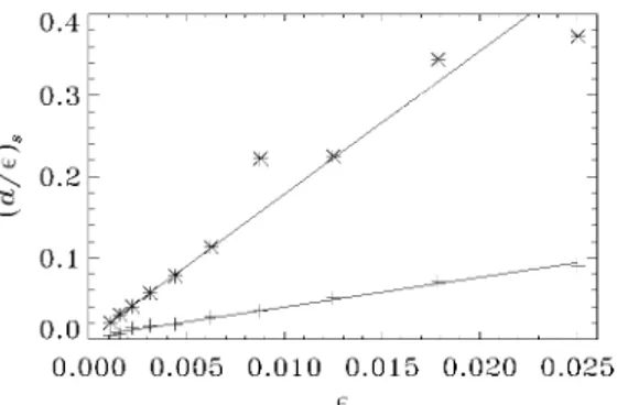
Fig. 5. Stationary relative error [d/e)s against e. Plus symbols correspond to a = 0.75, UJ = 0.5 (slope 3.6±0.1); and asterisks to a = 0.5, w = 2 (slope 18 ± 1).

t h e fact t h a t p a t t e r n s with smaller length scales appear for a = 0.5, u> = 2 (see Fig. 1).

An experimental confirmation of t h e CSH equation would require t o know a specific value of t h e appropriate distance t o threshold for which t h e equation is valid. Let us suppose t h a t t h e sought experimental confirmation has a m a x i m u m relative error of f 0% and make t h e favorable assumptions t h a t t h e Maxwell Bloch equations accurately describe t h e experiment and t h a t t h e chosen p a r a m e t e r s correspond t o a simple p a t t e r n with characteristic length equal t o S^isp ~ 1 as, for example, for a = 0.75, LU = 0.5. Then, using t h e slopes of Figure 5, we can calculate t h a t t h e distance t o threshold should not exceed r — 1 = 0.003, and t h e p u m p must be t u n e d with a relative error smaller t h a n 0.3%. For a = 0.5, u> = 2, where p a t t e r n s with diffu-sive scale (5difi ~ i / e arise, t h e situation is worse since the m a x i m u m distance t o threshold is r — 1 = 0.0006, and the relative error of t h e p u m p should be smaller t h a n 0.06%.

4 Conclusions

We performed numerical integrations of t h e Maxwell Bloch equations and t h e corresponding CSH equation, for a class C laser. T h e CSH equation gives a simplified and reduced dynamics of t h e original Maxwell Bloch equations for small detuning. C o m p a r i n g t h e results produced by b o t h set of equations, we obtain an average relative error of t h e CSH equation solutions. T h e numerical results con-firm t h e following theoretical prediction: (d/e)s ~ e, where (d/e)s is t h e s t a t i o n a r y relative error t h a t is reached for long times (the small p a r a m e t e r e is introduced in the deduction of t h e CSH equation and is directly related to the detuning and distance t o threshold). Therefore, as ex-pected, t h e CSH equation with terms of different asymp-totic order [31] is t h e appropriate envelope equation to accurately represent t h e behaviour of t h e Maxwell Bloch equations when e —> 0. T h e behaviour (d/e)s ~ e was numerically reproduced in Figure 5 where two different slopes were obtained for two points in p a r a m e t e r space a-uj. T h e plot shows t h a t , as expected, t h e difference in-creases faster for a = 0.5 and u> = 2, i.e., for t h e more complex case where small diffusive scales are present.

Note t h a t t h e fact t h a t t h e CSH gives a good approx-imation of t h e MB for small deviations from t h e lasing threshold, |r — 1| ~ e2 <C 1, does not constitute any nov-elty; this is in fact an expected result since t h e CSH is precisely derived from t h e MB in t h e e —> 0 limit. W h a t constitutes t h e main point of this paper is t h e numeri-cal confirmation t h a t this CSH contains t e r m s of different asymptotic order, see [31]. This asymptotic nonuniformity of t h e CSH has been systematically overlooked in t h e lit-e r a t u r lit-e (slit-elit-e lit-e.g., [12,13]), and it is lit-esslit-ential in ordlit-er to correctly model t h e laser dynamics near threshold.

The numerical results also allow us t o estimate the distance t o threshold range for which t h e CSH equation holds. Assuming an average relative error of 10%, t h e max-imum distance t o threshold is between 0.003 and 0.0006 for t h e p a r a m e t e r values analyzed: a = 0.75, u> = 0.5, and a = 0.5, u> = 2. T h e most restrictive value (0.0006) corre-sponds t o t h e case when t h e resulting p a t t e r n has diffusive scales (Jdifi ~ i / e ) . Although it is not unfeasable t o ex-perimentally establish such small distance t o threshold, it requires a fine t u n i n g of t h e p u m p t h a t is not usually avail-able in s t a n d a r d lasers. Another i m p o r t a n t experimental difficulty is t o obtain a wide enough b e a m for t h e p a t t e r n s to develop.

Finally, it is i m p o r t a n t t o mention t h a t , despite of the problems for setting u p an accurate laser experiment in the CSH range, t h e numerical results on this paper confirm-ing t h e validity of t h e CSH equation are interestconfirm-ing and valuable from t h e more general point of view of P a t t e r n Formation. T h e CSH equation is an envelope equation and it is universal in t h e sense t h a t its s t r u c t u r e depends only on t h e kind of instability of t h e problem and not on the particular physical problem under consideration.

This work has been supported by AECI (Agenda Espafiola de Cooperacion Internacional), Spain, under grant PCI A/6031/06. M.H. acknowledges Consejo Nacional de In-vestigaciones Cientificas y Tecnicas (CONICET, PIP 5666, Argentina) and ANPCyT (PICT 2004, N 17-20075, Argentina) for partial support. The work of C M . has been supported by the Spanish Ministerio de Educacion y Ciencia under grant MTM2007-62428, by the Universidad Politecnica de Madrid under grant CCG07-UPM/000-3177, and by the European Office of Aerospace Research and Development under grant FA8655-05-1-3040.

References

M. Cross, P. Hohenberg, Rev. Mod. Phys. 65, 851 (1993) J. Swift, P. Hohenberg, Phys. Rev. A 15, 319 (1977) S. Longhi, A. Geraci, Phys. Rev. A 54, 4581 (1996) M. Santagiustina, E. Hernandez-Garcia, M. San-Miguel, A.J. Scroggie, G.L. Oppo, Phys. Rev. E 65, 036610 (2002) S. Hewitt, J.N. Kutzt, SIAM J. Appl. Dyn. Syst. 4, 808 (2005)

P. Manneville, Theor. Comp. Fluid Dyn. 18, 169 (2004) A. Buka, B. Dressel, L. Kramer, W. Pesch, Chaos 14, 793 (2004)

A. Golovin, B. Matkowsky, A. Nepomnyashchy, Physica D 179, 183 (2003)

K. Staliunas, M. Tarroja, G. Slekys, C. Weiss, L. Dambly, Phys. Rev. A 5 1 , 4140 (1995)

K. Staliunas, G. Slekys, C. Weiss, Phys. Rev. Lett. 79, 2658 (1997)

J. Lega, J. Moloney, A. Newell, Phys. Rev. Lett. 73, 2978 (1994)

J. Lega, J. Moloney, A. Newell, Physica D 83, 478 (1995) H. Risken, K. Nummedal, J. Appl. Phys. 39, 4662 (1968) L. Narducci, J. Tredicce, L. Lugiato, N. Abraham, D. Bandy, Phys. Rev. A 33, 1842 (1986)

L. Lugiato, C. Oldano, L. Narducci, J. Opt. Soc. Am. B 5, 879 (1988)

P. Coullet, L. Gil, F. Rocca, Opt. Commun. 73, 403 (1989) P. Jakobsen, J. Moloney, A. Newell, R. Indik, Phys. Rev. A 45, 8129 (1992)

A. Barsella, C. Lepers, M. Taki, P. Glorieux, J. Opt. B: Quantum Semiclass. Opt. 1, 64 (1999)

J.F. Mercier, J. Moloney, Phys. Rev. E 66, 036221 (2002) L.M. Narducci, N.B. Abraham, Laser Physics and Laser Instabilities (World Scientific Publishing, 1988)

D. Dangoisse, D. Hennequin, C. Lepers, E. Louvergneaux, P. Glorieux, Phys. Rev. A 46, 5955 (1992)

N.R. Heckenberg, R. McDuff, C. Smith,

H. Rubinsztein-Dunlop, M. Wegener, Opt. Quant. Elect. 24, S951 (1992)

E. D'Angelo, E. Izaguirre, G. Mindlin, G. Huyet, L. Gil, J. Tredicce, Phys. Rev. Lett. 68, 3702 (1992)

A. Coates, C. Weiss, C. Green, E. D'Angelo, J. Tredicce, M. Brambilla, M. Cattaneo, L. Lugiato, R. Pirovano, F. Prati, Phys. Rev. A 49, 1452 (1994)

G. Lippi, H. Grassi, T. Ackemann, A. Aumann, B. Schapers, J. Seipenbusch, J. Tredicce, J. Opt. B: Quantum Semiclass. Opt. 1, 161 (1999)

F. Arecchi, S.B.P Ramazza, Phys. Reports 318, 1 (1999) L. Lugiato, M. Brambilla, A. Gatti, Advances in Atomic, Molecular, and Optical Physics 40, 229 (1999)

K. Staliunas, V. Sanchez-Morcillo, Transverse Patterns in Nonlinear Optical Resonators, Springer Tracts in Modern Physics (Springer-Verlag, 2003)

A. Newell, J. Moloney, Nonlinear Optics (Addison Wesley Publishing Co., 1992)

C. Martel, M. Hoyuelos, Phys. Rev. E 74, 036206 (2006) G. Oppo, G. D'Alessandro, W. Firth, Phys. Rev. A 44, 4712 (1991)

P. Jakobsen, J. Lega, Q. Feng, M. Stanley, J. Moloney, A. Newell, Phys. Rev. A 49, 4189 (1994)

C. Canuto, H. Hussani, A. Quarteroni, T. Zang, Spectral Methods in Fluid Mechanics, Springer Series in Computational Physics (Springer-Verlag, 1988)

M. Frigo, S. Johnson, FFTW (available at