Structure and stability of the equilibrium set in potential-driven flow networks

Structure and stability of t h e equilibrium set

in potential-driven flow networks

R I C A R D O R I A Z A

Abstract

In this paper we address local bifurcation properties of a family of networked dy-namical systems, specifically those defined by a potential-driven flow on a (directed) graph. These network flows include linear consensus dynamics or Kuramoto models of coupled nonlinear oscillators as particular cases. As it is well-known for consensus systems, these networks exhibit a somehow unconventional dynamical feature, namely, the existence of a line of equilibria, following from a well-known property of the graph Laplacian matrix in connected networks with positive weights. Negative weights, which arise in different contexts (e.g. in consensus models in signed graphs or in Kuramoto models with antagonistic actors), may on the one hand lead to higher-dimensional manifolds of equilibria and, on the other, be responsible for bifurcation phenomena.

In this direction, we prove a saddle-node bifurcation theorem for a broad family of potential-driven flows, in networks with one or more negative weights. The goal is to state the conditions in structural terms, that is, in terms of the expressions defining the flowrates and the graph-theoretic properties of the network. Not only the eigenvalue requirements but also the nonlinear transversality assumptions supporting the bifurca-tion motivate an analysis of independent interest concerning the rank degeneracies of nodal matrices arising in the linearized dynamics; this analysis is performed in terms of the contraction-deletion structure of spanning trees and uses several results from ma-trix analysis. Different examples illustrate the results; some linear problems (including signed graphs) are aimed at illustrating the analysis of nodal matrices, whereas in a nonlinear framework we apply the characterization of saddle-node bifurcations to networks with a sinusoidal (Kuramoto-like) flow.

1 Introduction

This paper addresses certain qualitative properties of potential-driven flows defined on net-works. From different perspectives, this kind of problems have been addressed in many application fields, which include coupled oscillators, operations research, circuit theory, elec-tronic engineering, water and gas networks, power systems, traffic networks or multiagent systems, to name but a few: cf. [2, 3, 9, 10, 11, 16, 21, 26, 27, 28, 32, 34, 37, 42, 48]. Our point of view is deliberately a general one, as we aim to explore in structural terms certain proper-ties of dynamical systems defined on networks, without focusing on specific models coming from applications; in our analysis we examine systematically the way in which the dynamical processes interact with the graph-theoretic underlying structure, looking for general results except for the fact t h a t the dynamics is assumed to be defined by a potential-driven flow. Very broadly speaking, this approach has been systematically exploited in nonlinear circuit theory in the last decade [29, 39]: our present goal is to extend somehow this perspective to the study of certain aspects of complex network dynamics, which define a very active topic research (see the works cited above and references therein). From this point of view the scope of potential applications of our results is rather wide.

Specifically, we are interested in the fact t h a t potential-driven flows systematically yield non-isolated equilibrium points. This is well-known for instance in the context of so-called consensus protocols [34, 37, 44], where lines of equilibria arise pervasively. These consensus protocols can be easily reformulated as a potential-driven flow in a network of cooperating agents: find details in Section 2. The one-dimensional nature of the equilibrium set can be understood as a consequence of the structure of the (positively) weighted Laplacian matrices arising in these models; here the positive weights reflect the fact t h a t agents cooperate in the sense that they tend to reach a common position; alternatively, this model can be seen as a redistribution system in which a flow evolves in a way such t h a t all agents asymptotically get the same quantity of a given commodity or resource.

weighted matrix-tree theorem; these results, whose origins go back to the pioneering work of Kirchhoff and Maxwell, will be placed in the appropriate context by examining additionally several related recent works [6, 9, 10, 13, 46, 47].

Potential-driven flow networks include in particular a wide family of Kuramoto models (cf. [2, 16, 23, 26, 28, 42, 45]) and we will show, specifically, that our saddle-node bifurcation characterization applies to certain networks with a sinusoidal (Kuramoto-like) flow, extend-ing some results from [16]. This, together with some additional examples concernextend-ing flows in signed graphs, can be found in Section 5. Finally, Section 6 compiles concluding remarks and lines for future research.

2 Potential-driven flows in networks

Networks will be assumed in this paper to be defined by a directed graph (or digraph) without self-loops. For the sake of simplicity we assume throughout the document that the digraph is connected and that it has at least one edge. Denoting by n and m the number of nodes and edges, respectively, define the incidence matrix A = (a¿j) G Rraxm entry wise by

(

— 1 if edge j enters node i (1)

0 if edge j is not incident with node i.

2.1 Flows

A flow on such a network is defined by a dynamical system of the form

5oX' = -Au, (2)

where 5 = (5\,..., 5n) G Era, with entries 5i G {0,1}; x = (x\,..., xn) G Era is the state

vector, with each component modelling the state of a single node, whereas u = (u\,..., um) G

Rm is a vector of flowrates. The circle o stands for the Hadamard product, so that each component within the left hand-side amounts to the product bix\ and therefore (2) reads componentwise as

Six'i = —AiU, i = 1 , . . . , n, (3)

where Ai is the i-th row of the incidence matrix A.

To fix ideas, consider a simple connected network in which a given resource (e.g. electrical charge, water, gas, a given commodity, etc.) flows among a set of n agents located at the network nodes; here "simple" means that the network has neither parallel edges nor self-loops. Let us first assume that all agents collect this commodity (this corresponds to choosing

5i = 1 for i = 1 , . . . , n), and denote the amount of the collected resource at node i by x¿.

to i). Equation (3) just expresses, with 8i = 1, that the increase x\ of the stored resource at node i equals the net flow entering the node, t h a t is, — AiU with the sign convention above.

Cases in which some Si's do vanish model situations in which some nodes do not accu-mulate the aforementioned resource, yielding problems with so-called partial storage. Both types of nodes (those with Si = 0 and with 8i = 1) may well be present in flow networks and note t h a t (3) describes the continuity equations for both. If all Si's do vanish we arrive at a widely studied framework stemming from the work of Ford and Fulkerson (cf. [5, 15]). From another perspective, the vanishing of all Si's happens naturally in electrical circuit theory, u standing in this case for the electrical current and (2) (which amounts in this context to Au = 0) expressing Kirchhoff's current law.

For the sake of simplicity, we will focus on cases with 8i = 1 for i = 1 , . . . , n. In this setting, (2) is simply

x1 = -Au. (4)

In this generality, flow networks arise in many different application fields: let us mention for example distribution networks [11, 14, 27, 43], supply chains [17], traffic networks [10, 21], power systems [9, 18], inventory systems [4, 8], etc. We do not at all attempt to be exhaustive, and references are only a small sample of a huge amount of literature. Worth mentioning are also the works [10, 27], aimed at providing very general dynamic models for network flows. Depending on the application field, other (related) models can be found in the literature. For instance, the form of (4) above assumes that the so-called node divergence di = —Am (see e.g. [10]) equals the change in the stored resource at node i; in other cases, e.g. in the presence of external supplies or demands, the right-hand side of (4) takes the form —Au + s for a (possibly time-dependent) vector s = (s\,..., sn) of supply/demands (cf. for instance [8, 10, 14, 43]). When supplies and demands are balanced we have Y17=i Si = ® a nd> using

basic properties of the incidence matrix, this makes it possible to recast the vector field above as — A(u + s) for a certain vector s, driving the system to the form (4). We refer the reader to the aforementioned papers for additional details regarding these and other flow network models.

2.2 P o t e n t i a l - d r i v e n flows

System (4) is underdetermined. The way in which the flowrates u interact with the node state variables x may be defined from different perspectives; for instance, in a game-theoretic setting the agents' strategies would define the flows, or in the framework of control theory u might be designed as to achieve a given goal. Here we will assume t h a t the flowrates u are explicitly defined in terms of the node states x by a relation of the form

u = f(ATx), (5)

where / : Rm —>• Rm is a possibly nonlinear, differentiable map which is assumed to have a diagonal structure, that is

with fj : IR —>• IR depending only on ( AT) J X ; here (AT)j is the j - t h row of AT. This means that the flowrate in edge j (connecting nodes i and k) depends only on the difference x¿ — Xk- We emphasize that, implicitly, there are two modelling assumptions here; first, the flowrate Uj on the j - t h edge depends only on an edge-supported variable Q and, second, this variable is defined from the states at the incident nodes simply as the difference Xi — Xk- The variables

x can be then thought of as a potential and hence the "potential-driven" label for these

flows: electric potential or pressure are examples in electrical circuits and water networks, respectively (see [10, 27, 32]). In the electrical circuit framework, Q = Xi — Xk is called the voltage drop or simple the voltage at the j - t h edge. Note that, by construction, the above defined variables ( verify B( = 0 for any cycle matrix B (see e.g. [5, 39]), an identity which in the electrical circuit context is Kirchhoff's voltage law and defines the dual relation of the equation Au = 0 mentioned above; in this direction, further duality relations are discussed in an abstract setting in [10].

The assumptions above transform (4) into

x' = -Af(ATx), (6)

which defines a general formulation for potential-driven flows in networks. The focus of this paper is on systems of the form (6) (and its parameterized version (27)), with the restrictions on / just mentioned.

2.2.1 Linear consensus protocols

A simple example is obtained if u is designed in order to get a fair (equal) distribution of the aforementioned commodity among all agents. This can be achieved by setting the (potential-driven) form for the flowrates u = ATx, which is just a redistribution law in which the flow from i to k equals Xi — Xk- In this setting (6) is just

x1 = -hx (7)

where L = AAT is the graph Laplacian matrix. The dynamics of (7) has been analyzed in the context of so-called consensus protocols [34, 37, 44], and the state variables x may be checked to converge to a common value which is the arithmetic mean of the initial values

x\(0),... ,xn(0). This means that the resource is indeed redistributed among all the agents in a way such that all of them asymptotically store the same quantity.

Note that the right-hand side of (7), defined by the Laplacian matrix AAT, can be un-derstood as a particular instance of the product AWAT with W = Im. Actually, the essential features of (7) are preserved if the product AAT is replaced by the weighted Laplacian matrix

Ar, and we will use the term "reduced nodal matrix" for A-W/L7; note also that in the

literature the term "nodal matrix" often refers to the latter).

Things will change in the presence of so-called antagonistic actors or contrarians, dis-playing a negative weight in their connection (see [6, 13, 46, 47] or [23, 45] in the context of Kuramoto models). Although this will be discussed in Section 3, it is worth remarking here another closely related research direction on linear consensus systems which has been recently developed [3, 33]. Given a set of agents including some antagonistic pairs, one may define the coefficient matrix of (7) in a different manner in order to retain (in a certain sense) the convergence properties of the positively weighted case; this is supported on alternative definitions of the Laplacian matrix for negatively weighted networks and signed graphs (cf.

[25] and references therein). This approach is followed in [3], where the author sets the coef-ficient matrix as L = — C + D, C being (as in the standard weighted Laplacian matrix) the weighted adjacency matrix, but now the entries of the diagonal matrix D being defined by the sum of the absolute values of the weights (whereas in the standard definition of the weighted Laplacian matrix, the weights retain their signs in the sums which define D). In signed graphs, this amounts to combining the weighted or signed adjacency matrix C with the (say, "unsigned") degree matrix D, contrary to the standard weighted Laplacian matrix where D turns out (always in the signed framework) to be equivalent to the so-called signed degree matrix (cf. [25]). This alternative notion yields the standard weighted Laplacian matrix in positively weighted networks, but allows for a nice extension of the convergence properties mentioned above to cases with negative weights; namely, the network is shown in [3] to reach a bipartite consensus, meaning that all nodes asymptotically reach the same absolute value, if and only if the graph is structurally balanced, that is, iff it admits a splitting of the nodes into two groups with all positive (resp. negative) connections occurring inside each group (resp. between both groups); moreover, the sign of the consensus value is the same within each group, and differs from one group to another. Find some very recent extensions of these results in [33]. It is important to note that, in contrast, the results addressed here for linear problems are always directed to the standard weighted Laplacian matrix.

2.2.2 Nonlinear problems, Kuramoto models

An important family of networked nonlinear dynamical systems (namely, Kuramoto-like models for coupled oscillators) defines another instance of a potential-driven flow, as detailed in what follows. It is worth emphasizing that these systems have driven much research in this area. In its original formulation [28], the Kuramoto model reads as

k <A

9 • = cui } sin(6>¿ -9j), i = l,...,n, (8)

where 6i lies on S1, u;¿ are the natural oscillator frequencies, and k is the coupling strength.

strength is the same in all edges. By relaxing these assumptions, one gets (cf. [26])

e¡ = UÍ - AtWs(AT9), i=l,...,n, (9)

where, as in (3), A¿ is the i-th row of the incidence matrix; W is a diagonal matrix whose j - t h diagonal entry is the coupling strength in the j - t h edge, and the map s just denotes the product sin x i™} x sin. Note in particular that the coupling strengths (or weights) may in some cases take negative values, as discussed in [23, 45]. By means of the linear coordinate change

Xi = 9i- cust, tus = —%=l \ i= 1 , . . . , n, (10)

n

the model (9) takes the form

x'i = üJi- AiWs(ATx), i = 1 , . . . , n, (11)

with UJi — UJi — UJg. Note that UJS = ———- is the synchronization frequency (see e.g. [16])

_ n

and that, by construction, Y17=i ^í = 0. Because of the form of the incidence matrix A, the latter can be checked to imply that the vector ÜJ = (üj\,... ,ÜJn) belongs to imA and makes it possible to recast (11) as

x1 = -A(v + Ws(ATx)), (12)

for a certain vector v which is uniquely defined in imAT. System (12) has the form depicted

in (6) and this means that Kuramoto models in arbitrary topologies and with arbitrary coupling coefficients can be written as a potential-driven network flow in the coordinate system defined by (10). Therefore, later results apply in particular to Kuramoto-like models; in this direction, with illustrative purposes we will show how the saddle-node bifurcation characterization obtained in Section 4 applies to flow networks with a sinusoidal flowrate.

3 On the equilibrium set of potential-driven flow networks

3.1 Equilibria and t h e s u b i m m e r s i o n t h e o r e m

For notational simplicity we denote by g(x) the right-hand side of (6), t h a t is,

g(x) = -Af(ATx). (13)

It is easy to check t h a t equilibria of (6) may never be isolated; indeed, provided that g(x) vanishes for a given x*, then x = x*+v also annihilates g(x) = — Af(ATx), for any v G ker AT. Note t h a t this kernel is never trivial, being one-dimensional in a connected digraph (since in this case rk A = n— 1, cf. e.g. [5, 12]). In general, we do not require / to be linear; of course, when / is a linear map the equilibrium set is a linear manifold. The problem we address in this section is the characterization of the cases in which the equilibrium set is locally a line, as it happens for (7), as well as some problems with a minimal degeneracy, namely, those in which the corank of the weighted Laplacian matrix does not exceed two; this will be used in the saddle-node bifurcation analysis of Section 4.

We will make use of the subimmersion theorem, which states that if Q is an open subset of Era, and g is a smooth mapping Q —>• W such t h a t the Jacobian matrix g'(x) has constant

rank r < p on Q, then for every y in g(Q) the set g~l(y) is a submanifold of Q with dimension n — r (see e.g. Th. 3.5.17 in [1]). The result also holds if g has constant rank r on a neighborhood of g^iy). We will use this result with g given i n ( 1 3 ) , y = 0 , p = n and r = n — 1 to characterize the problems in which the equilibrium set is a line around a given equilibrium point x* (more precisely, to rule out other nearby equilibria apart from those spanned by ker AT). The Jacobian matrix g'(x) reads as

g\x) = -Af'(ATx)AT (14)

and, since rkA = n—l,lt follows t h a t g'(x) is persistently rank deficient. Therefore, for the equilibrium set of (6) to be one-dimensional (at least locally around x*), it is enough to derive conditions guaranteeing rk g'(x*) = n — 1, since this maximum rank would necessarily be attained also on a neighborhood of x*. In order to examine the rank of g'(x*), let us denote the derivatives of the components of / at

and let W stand for the diagonal matrix with entry Wj in the j - t h diagonal position: be aware of the assumption that fj depends only on (j = (AT)jX. With this notation we have

g\x*) = -AWAT. (16)

This expression shows t h a t the Jacobian matrix g'(x*) has the structure of a weighted Lapla-cian matrix, with weights being defined by the derivatives dfj/dQ at ATx*.

3.2 P o s i t i v e w e i g h t s

If all weights Wj (that is, all derivatives dfj/dQ) are positive at ATx*, then it is a simple matter to check t h a t

Indeed, just note that AWATv = 0 implies vTAWATv = 0 and therefore ATv = 0 because of the positiveness of the diagonal matrix W. The relation depicted in (17) implies that

rkg'(x*) = rk AWAT = rk AT = n — 1 and, because of the subimmersion theorem, it follows that equilibria actually define a line near x*. This also underlies the existence of an equilibrium line in linear consensus systems such as (7).

3.3 Negative weights: non-degenerate cases

If W in (16) includes negative entries, the remarks just stated do not apply, and we may actually find potential-driven flow dynamics on connected graphs displaying higher (> 2) dimensional manifolds of equilibria. This may of course be the case even in linear problems: examples in a linear context, involving signed graphs, can be found in subsection 5.1 below. A different approach is needed to analyze the structure of the equilibrium set in digraphs with possibly negative weights. In this setting, the main result is the weighted matrix-tree theorem (see e.g. [5]), according to which the non-singularity of the reduced nodal matrix arising below can be characterized in terms of a determinantal expansion defined by the spanning trees of the (assumed connected) graph. This approach can be traced back to the work of J. C. Maxwell and, in the dual setting, to that of Kirchhoff (cf. [12, 38]). In the network context this approach has been used in [6] (see also [13, 46, 47]). Together with the subimmersion theorem, this yields a simple characterization of the cases in which equilibria locally define a line; this is stated in Proposition 1 below, where we make use of the notion of the weight of a spanning tree; this is simply the product of the weights of the tree edges.

Proposition 1. Assume that the dynamical system (6) is defined on a connected digraph.

The Jacobian matrix g'(x*) in (16) has corank one if and only if the sum of the spanning tree weights does not vanish, where the edge weights are given by (15). If this sum is not null, then the set of equilibria is a line locally around the equilibrium point x*.

Proof. The matrix AWAT in the right-hand side of (16) is a weighted Laplacian matrix, which is rank deficient since rkA = n—l. According to the weighted matrix-tree theorem, we know that this matrix actually meets the maximal rank n — 1 if and only if

det(AYWAj) ^ 0, (18)

for an arbitrary choice of a reduced incidence matrix AT, defined by any set of n — 1 rows of

A (without loss of generality, in what follows we are allowed to work e.g. with the reduced

incidence matrix Ar defined by the first n— 1 rows of A). Moreover, the determinant in (18) is known to admit a Cauchy-Binet determinantal expansion [24] of the form

det(A

WAj) = J2Tl

J> (

)

Ar stands for the reduced incidence matrix of a spanning tree. The weighted matrix-tree theorem then guarantees t h a t g'(x*) has corank one if and only if the sum of the spanning tree weights does not vanish.

Provided t h a t the non-vanishing condition (18) holds, the identity rkg'(x*) = n — 1 yields, as a direct consequence of the subimmersion theorem in the terms stated above, a

local one-dimensional structure for the equilibrium set near x*. • Proposition 1 provides a graph-theoretic characterization, in terms of the digraph tree

struc-ture, of the problems which systematically lead to lines of equilibria in potential-driven flow networks with (possibly) some negative weights. In this direction, it is worth remarking that in the network dynamics literature [46, 47] (see also [13], where a different proof of the main result in [46] is given), the vanishing requirement in the sum of tree weights (19) is implicitly reported to be responsible for the increase in the multiplicity of the null eigenvalue and, accordingly, for the loss of semidefiniteness of the Laplacian matrix beyond the so-called effective resistance obtained after recasting the network in electrical circuit terms, weights playing the role of conductances; note in this regard that Maxwell's determinantal expan-sion implicitly supports the effective resistance notion used in the aforementioned papers (see also the remarks preceding Lemma 1). In our setting, the failing of the aforementioned non-vanishing requirement in the sum of tree weights, together with the appropriate transver-sality assumptions, will be responsible for bifurcation phenomena in nonlinear problems, as detailed in Section 4.

Certainly, if all weights are positive then the sum arising in Proposition 1 is positive and therefore non-null, because all tree weights are positive. This is of course consistent with the discussion of subsection 3.2 regarding the one-dimensional nature of the equilibrium set in positively weighted networks, for which there is no need to use these tree-based tools.

3.4 N e g a t i v e w e i g h t s : m i n i m a l d e g e n e r a c i e s

Degenerate problems (defined by the singularity of the reduced nodal matrix ATWAj or, equivalently, by the vanishing of the determinantal expansion (19)) may well arise in the presence of negative weights. In this context it is important to characterize minimal degen-eracies, t h a t is, minimal rank drops in the reduced nodal matrix; this will be a key element in the saddle-node bifurcation analysis of Section 4, but also has an impact in the structure of the equilibrium set of (linear or nonlinear) potential-driven flow networks. Some problems with minimal degeneracies are characterized below, again in terms of the structure of the graph spanning trees. As usual, if M is an n x m matrix, c o r k M stands for n — rk M. P r o p o s i t i o n 2. Assume that the reduced nodal matrix ATWAj of a weighted connected di-graph is singular. Then cork(ArW/lJ) = 1 if there is an edge e for which at least one of the

following conditions hold.

(a) The sum of products of all tree weights but We, extended over the set of spanning trees which include e, does not vanish.

do not include e, does not vanish.

(c) All weights but We do not vanish and have the same sign.

Proof. The three statements are essentially a consequence of Jacobi's identity, which

ex-presses the derivative of the determinant of a (smoothly) parameter-dependent matrix as

-f- (det Mia)) = tr ((Adj M(a))^M(a)] ,

da \ da J

see e.g. [19, 31]. Provided that M(a) is a singular matrix at a given a, an elementary property of the adjoint matrix (namely, the transpose of the matrix of cofactors) says that Adj M(a) ^ 0 if and only if cork M(a) = 1. It then follows that

d

det Mia) = 0, — (det Mia)) ^ 0 => corkM(cu) = 1. (20)

da

Below we apply this result to M = ArWAj, with We playing the role of the parameter a. To do so, in the determinantal expansion (19) we group together all the terms which involve We on the one hand, and those which do not on the other. This yields

det(AYWAj) = Kl{W)We + KQ(W), (21)

where W stands for the diagonal matrix defined by all weights except We. Note that, by construction, K\(W) is the sum of products of tree weights, exception made of We, extended over the set of spanning trees which include e, whereas K0(W) is, correspondingly, the sum of products of tree weights extended over the set of spanning trees not including e. Explicit expressions for K\(W) and K0(W) will be given later (cf. Remark 2).

Item (a) then follows from (20), since (21) obviously yields d det(ArWAj)/dWe = Ki(W), and the non-vanishing assumption in item (a) (i.e. K\{W) ^ 0) implies the minimal rank drop on ArWAj. In turn, the requirement in item (b) (which can be written as KQ(W) ^ 0) actually implies the one in (a), since the singularity of ArWAj means det(ArW//lJ) = 0,

and (21) then shows that K0(W) ^ 0 necessarily implies K\(W) ^ 0 (besides We ^ 0, a condition not used at this point). Finally, under the requirement depicted in (c), K\(W) cannot vanish (and hence (a) applies again) because this coefficient is constructed as the sum of non-vanishing terms with equal signs: note that these terms are products of a fixed

number of factors, all of which have the same sign. •

Remark 1. Item (c), in which We may vanish or not, is of interest in particular when there is exactly one negative weight (i.e. when We < 0 and the remaining weights are positive). In this setting the minimal rank drop can be also derived as a consequence of the results proved in [6], characterizing the number of positive/negative/null eigenvalues of nodal matrices in terms of the number of connected components c+ (resp. c~) of the subgraphs defined by

all nodes and the edges with positive (resp. negative) weights. Specifically, for the reduced nodal matrix ArWAj, Theorem 2.10 in [6] implies that the corank is bounded above by

c+ = 1, provided that the edge with a negative weight is not a bridge (should it be a bridge,

it would enter all spanning trees and hence yield a common factor in the expansion (19); since this would be the unique negative weight, the other factor in the expansion would be positive and this would preclude the singularity of the reduced nodal matrix). We then have

n + I — c~ — c += l and the corank-one condition follows. Note, however, that item (c) as

stated above also applies to cases with We = 0, which may well bifurcation value in certain situations (cf. Section 5.2).

Remark 2. It is worth providing explicit descriptions for the coefficients K\(W) and K0(W) in (21); these expressions are not explicitly needed in the proof of Proposition 2 but will be used later (cf. Section 4). To achieve that, let us (for ease of notation and w.l.o.g.) assume that e is numbered as the first edge, so that We = W\, and split

A

=

( i

i

)

,

(22)

where Ar (resp. AT) stands for the submatrix defined by the first column (resp. the last m— 1 columns) of AT. Hence Ar describes the incidence of edge e. We may then write

AYWAj = WxÁ.Á] + ÁVWÁ¡ (23)

(recall that W\ is a scalar). Remark that the first matrix in the right-hand side is a rank-one perturbation of the second one, and let us then apply the identity

det(uvT + M) = vTAdjMu + det M (24)

(cf. e.g. [31]) with u = WXAT, vT = ÁJ, M = ÁYWÁJ to derive

det(AYWAj) = H / i ir TA d j ( irH / ir T) ir + det(ÁYWÁJ), (25)

so that

KX{W) = Á]Adj(ÁYWÁ])ÁY (26a)

KQ(W) = det(ÁYWÁJ). (26b)

These descriptions provide a way to obtain the values K\ and K0 without the need to compute the whole set of spanning trees and their weights. This will be useful for instance in the computation of the bifurcation values arising in Theorems 1 and 2.

Additionally, these expressions reflect well the contraction-deletion recursive structure of spanning trees. Specifically, the identity K0(W) = det(ArWAj) expresses the fact that the set of spanning trees which do not include the edge e in the original graph (defining

KQ(W)) is exactly the set of spanning trees of the "deleted" graph obtained after removing e, provided that this edge is not a bridge (so that this deleted graph is connected). The reduced nodal matrix of this deleted graph is ArWAj (this is easily seen once we note that Ar is the incidence matrix of the graph obtained after removing e), consistently with the expression det(ArVyAj) in the right-hand side of the identity above. This idea will be

4 Saddle-node bifurcations in networks with negative weights

We now drive our attention to a parameterized version of (6), t h a t is, to dynamical systems of the form

x' = -Af(ATx,/i), (27)

with ¡i G E and / essentially satisfying the restrictions indicated in Section 2 (details are given later). We will focus on an equilibrium x* at a given parameter value // = //*, in order to examine dynamical phenomena in cases in which not all weights (arising from the linearization of the right-hand side of (27)) are positive. Denote g(x,fj) = —Af(ATx,fi).

In this setting, local bifurcation phenomena should be expected if / has the appropriate form. Among the bifurcations of equilibria, the saddle-node bifurcation is generic (in the sense specified in [41]) in one-parameter systems displaying a simple zero eigenvalue. There-fore, it is natural to check which conditions on / may result on saddle-node bifurcations in flow network dynamics of the form (27). Needless to say, we need / to be nonlinear, and its linearization at equilibrium to depict at least one non-positive weight, since otherwise the stability transition along the equilibrium branch predicted by the classical saddle-node bifurcation theorem (cf. the original paper [41] or [20, 36]) is easily ruled out.

4.1 A single n e g a t i v e w e i g h t

A first step in this direction is Theorem 1 below, which captures minimal conditions on / yielding indeed a saddle-node bifurcation. Theorem 2 in subsection 4.2 will extend this result to a broader setting (accommodating multiple negative weights). In Theorem 1, we will work in the scenario defined by the hypotheses on the vector field / stated below, which extend the ones considered in Section 2. Without loss of generality we assume that the edge accommodating the nonlinear flowrate is the first one and, accordingly, we denote by A the first column of A, so t h a t (AT)i = AT.

(a) The flowrate f\ depends smoothly on (ATx,fi).

(b) The remaining components fj (j = 2 , . . . , m) are independent of the parameter ¡i and depend linearly on (AT)jX, t h a t is,

fj((AT)jx,fji) = Wj(AT)jx, j = 2,...,m. (28)

More precisely, in (a) we assume t h a t f\ is twice differentiable. We will denote the first scalar argument of f\ as (\ (that is, f\ = /i(Ci >/•*)); recall t h a t (\ = ATx because of the potential-driven assumption. With this notation, the first weight will be

Wl{x,li) = ^{ÁJx,li) (29)

(c) The weights Wj are positive for j = 2 , . . . , m.

In this setting, the vanishing of the determinantal expansion (19) is the key requirement in the saddle-node bifurcation result stated in Theorem 1. Besides this condition, the result follows from standard assumptions on the nonlinear component f\; notably, no requirements on the network topology are necessary (this could be different in other settings, as subsection 4.2 or the last example in Section 5 illustrate). Consistently with the nature of potential-driven flows, the bifurcation does not yield a splitting of a single equilibrium but of a line of equilibria.

T h e o r e m 1. Assume that x* is an equilibrium of (27) at a given parameter value ¡i = ¡i*. Let the hypotheses (a), (b) and (c) on the components of f stated above hold and assume, additionally, the following.

df

1. The weight WI(X*,/J,*) = ——(ATx*,fi*) satisfies the identity

^(ftvi = -=MU% = -MS, pe)

SO E

T , n

i > W¡ KfiV)'

where T0 (resp. T\) is the set of spanning trees which do not include (resp. do include)

the first edge.

2. The component f\ additionally verifies

^ (iV,¿/) ^ o, ^ (iV,//) ^ 0. (31)

Then (27) has a (locally) unique equilibrium line comprising x* at ¡i = ¡i*. This equilibrium line bifurcates into two as ¡i undergoes the value ¡i*. Both bifurcating lines are normally hyperbolic: one of them is an exponential attractor whereas the other one is unstable.

Note that the linearization of a vector field at an equilibrium which is embedded into an equilibrium line necessarily depicts a zero eigenvalue. The line of equilibria is said to be normally hyperbolic if the remaining eigenvalues are away from the imaginary axis [30]. If all the remaining eigenvalues have negative real parts, then the line of equilibria attracts exponentially nearby trajectories. This is a consequence of the Sositaisvili-Palmer theorem

[35, 40]. Indeed, the dynamics on the equilibrium line is trivial (i.e. it reads x' = 0 for a scalar variable x parameterizing the equilibrim line, which is a center manifold): according to the aforementioned theorem, the local dynamics is then topologically equivalent to the system x' = 0, y' = Hy with all the eigenvalues of H having negative real part (H is the hyperbolic part of the linearization at equilibrium). Find details in the original papers [35, 40] or e.g. in [20, 30, 36].

W2, • • •, Wm; now W\ stands for We in (21). The statement of Theorem 1 implicitly uses the fact that Ki(W) does not vanish, since it is a sum of positive terms. Additionally, the proof will make use of some auxiliary results which are stated in advance.

The first one, stated in Lemma 1, is an extension of item (c) in Proposition 2 showing that with only one non-positive weight (that is, negative or null), then not only the rank deficiency of the reduced nodal matrix is at most one but actually only one eigenvalue may eventually become negative. We emphasize that this result is essentially known in the literature: cf. the work [6] referred to in the proof but also [46, 47] and [13] (the latter references focus on the loss of definiteness of the reduced nodal matrix at the critical parameter value, but the fact that locally beyond that value only one eigenvalue becomes negative follows naturally). Recall that Ar is the reduced incidence matrix defined by the first n — 1 rows of A.

Lemma 1. Consider a nodal matrix ATWAj of a weighted connected digraph, with W = diag(W/i,..., Wm). If W\ < 0 and Wi > 0 for i = 2 , . . . , m, then ATWAj has no more than

one non-positive eigenvalue.

Proof. Note first that if W\ = 0, the identity (23) easily shows that the claim is true,

because in this case ArWAj = ArWAj, and the latter is a symmetric positive semi definite matrix (note that W = diag(W/2, • • •, Wm) is positive definite). Since the rank deficiency of the former matrix is at most one, as shown in Proposition 2, it displays at most one non-positive (actually null) eigenvalue.

In the case W\ < 0 the result follows immediately from [6, Th. 2.10], since according to this result the number of positive eigenvalues is bounded below by c~ — 1, where c~ is the number of connected components of the subgraph defined by all nodes and the edges with negative weights. In a connected graph with a single negative weight we have c~ = n— 1 and therefore the number of positive eigenvalues is not less than n — 2. Since the total number of eigenvalues of the reduced nodal matrix is n — 1, it follows that no more than one eigenvalue

may be negative or zero. •

The second auxiliary result is stated in Lemma 2 below, and will support the transversality hypotheses in the saddle-node bifurcation theorem (cf. also Remark 4 after the proof of Theorem 1). The last example in Section 5 will show that this result does not hold trivially, since (32) may not be true in problems with more than one negative weight if no additional assumptions are imposed.

Lemma 2. Consider, as above, the reduced nodal matrix ArWAj of a weighted connected

digraph, with W = diag(Wi,..., Wm), W\ < 0 and Wi > 0 for i = 2 , . . . , m. If ArWAj is

singular, then

ir i imATWAj, (32)

where Ar stands for the first column of Ar.

therefore Ajv = 0 by orthogonality. Multiplying (23) by v we then get

ÁrWÁ¡v = 0 (33)

and therefore Ajv = 0 because W is positive definite. Together with Ajv = 0, this yields Ajv = 0, which is a contradiction because v ^ 0 and the columns of A J are linearly

independent (since Ar has maximal row rank). This completes the proof. • R e m a r k 3. For later use, it is worth emphasizing the (pretty obvious) fact that (32) is

equivalent to Ajv ^ 0 for any non-vanishing vector v in the one-dimensional kernel of ATWAj, since this will be helpful in order to unravel the geometrical meaning of the second order condition involved in Theorem 1 (cf. Remark 4).

Finally, in the proof of Theorem 1 (and also in Theorem 2) we will use a reduction of the dynamics of (27) to an invariant hyperplane, as stated below.

L e m m a 3. System (27) has a family of invariant hyperplanes of the form X\ + . . . + xn = k. By setting k = k*, y¿ = x¿, i = 1 , . . . ,n — 1 and E = ( X - i + l n - i l ^ _ i ) , where 1 is the vector of 1 's in Rnxl, the dynamics on the invariant hyperplane X\ + . . . + xn = k* reads as

y> = -AJiAjEy + Alk*^). (34)

Here Ar (resp. An) stands for the first n — 1 rows (resp. the last row) of A.

Proof. This is supported on the identity 1TA = 0, which expresses the fact that the sum of all rows of the incidence matrix A vanishes. From (27) it follows that lTx' = 0, that is,

J2x'i = 0, so that conserved quantity, to be denoted by k. This defines a set of invariant hyperplanes. The dynamics on any of them is easily described by means of

the linear change of coordinates given by y¿ = xi} i = 1 , . . . , n — 1, k = After elementary computations, in the coordinates z = (y,k) the system reads

y' = -AJ(ATBz,ii) (35a)

k' = 0, (35b)

where, as defined earlier, Ar stands for the first n — 1 rows of A, and

is the matrix yielding the change of coordinates x = Bz. We have made use of the identities

•-te':)—©

Equation (35a) admits further simplification. Indeed, write

A B = [AY An) I I = [AY — Anln_1 An) ,

and note that the identity 1TA = 0 can be recast as An = — l^_1Ar. This yields

ATB = (AJ (!„_! + In-ill-!) Al) . (36)

In light of (36), the reduced system (35a) can be written on the invariant hyperplane

x\ + . . . + xn = k* in the form depicted in (34) and the claim is proved. •

For later use we emphasize that E, as defined in Lemma 3, is a symmetric positive definite matrix.

Proof of Theorem 1. The proof of Theorem 1 will make use of Proposition 2 and Lemmas

1, 2 and 3, and proceeds in three steps.

1. First we show that the reduction (34) arising in Lemma 3 has an equilibrium y* which undergoes a saddle-node bifurcation at ¡i = ¡i*. Fix k* = x\ + . . . + x*n and denote by

F(y, k*, ¡i) the right-hand side of (34), that is,

F(y, k*,fi) = -Af(AjEy + AJnk\^).

The fact that y*, defined componentwise by y* = x*, i = 1 , . . . , n — 1, is an equilibrium point of (34) follows trivially from the assumption that x* is an equilibrium of (27). We then need to check that the conditions supporting the saddle-node bifurcation theorem (cf. [20, Th. 3.4.1] or [36, Th. 1 in §4.2]) do hold for (34); namely, we need to show that

(i) Fy(y, k*, ¡i*) has a simple null eigenvalue, and no other purely imaginary eigenvalues;

iii) F,{y\k*^*) iimFy{y\k*^*)- (37)

(iii) Fyy(y*,k*,n*)vv£imFy(y*,k*,n*) (38)

do hold, being v a non-vanishing vector in kerFy(y*, k*,fi*). Subscripts are used here to denote differentiation.

Under the conditions above, Fy(y*, k*, ¡i*) takes the form

Fy(y*,k*,/i*) = -AJc(AjEy* + ATnk*, ¡i*)Aj E = -ArWAjE,

where the notation W is used to describe the diagonal matrix defined by the entries W\(x*, ¡i*) and W2, • • •, Wm given above. Except for the last factor E (which is non-singular), this matrix has the form examined in Proposition 1, and the identity (30) indicates that the determinan-tal expansion (19) vanishes (cf. (21)). This means that ArWAj and therefore Fy(y*, k*, ¡i*) have indeed a null eigenvalue. Additionally, taking the (unique) symmetric positive definite square root \JE of the (symmetric positive definite) matrix E (cf. Theorem 7.2.6 in [24]), by multiplying

by y/E from the left and ( \E\ from the right, the matrix ArWAjE is seen to be similar to

víEArWÁ¡víE. (39)

This matrix is congruent to ATWAj, which has a simple zero eigenvalue according to item (c) of Proposition 2. Therefore, this is also the case for ATWAjE, as we aimed to show. Also, the similarity to (39) precludes purely imaginary eigenvalues (other than zero).

The condition depicted in (37) (item (ii)) easily follows from Lemma 2 and the first condition in (31), once we note that the structure of / yields

FM( y * , r , ^ ) = - i r ^ ( i V , ^ ) , (40)

because only f\ depends on ¡i.

Regarding the second order condition (38) (item (iii)), we use the identity (23) and note that only W\ depends on y (actually, in the form W\ = W\(AjEy, ¡i)), so that

d

f

Fyy(y*,k*,fi*)vv = -Ar-^(ÁTx*,fi*)(ÁjEv)2 (41)

(mind that AjEv is a scalar). Using the fact that AjEv ^ 0 because Ev G kerA-W/L7

(cf. Remark 3), together with Lemma 2 and the second condition in (31), we conclude that condition (iii) is also met and therefore system (34) indeed undergoes a saddle-node bifurcation at (y*,¡j,*), as we aimed to show in the second step of the proof.

2. In item 1 above we have proved that y* experiences a saddle-node bifurcation (as ¡i varies) in the hyperplane defined by k*. This means that either for ¡i> ¡i* or ¡i < ¡i* two equilibria show up. We will generically denote both as yeq and the reader may distinguish them as yeqi and yeq2. As detailed in what follows, for ¡i close to ¡i* one of these is asymptotically stable

and the other one unstable, the latter displaying a one-dimensional unstable manifold. The linearization of F at such equilibria yeq is defined by the matrix

Fy(yeq, k*,fi) = -AJ¿Á¡Eyeq + AJnk\n)Á¡E = -ArWeqAjE,

where the notation Weq is aimed at indicating that the weight values (actually W\) depend on the equilibrium location. Following the reasoning above, the matrix ArWeqAjE only has real eigenvalues and has the same inertia as ArWeqAj. Since no weight apart from

W\ may be negative, no more than one eigenvalue of ArWeqAjE may then be negative, according to Lemma 1, and this means that the eigenvalue transition implied by the saddle-node bifurcation is necessarily a transition from the all-negative (i.e. asymptotically stable) case (mind the — sign in Fy) to a scenario with only one positive eigenvalue, as claimed above.

3. Finally, we show that for k ^ k*, equilibrium solutions y of

are, for any fi, in one-to-one correspondence with those of (34), to be denoted by yeq, via the relation

y = yeq + ^ ^ i n - i - (43)

n

Indeed, assume that y annihilates the right-hand side of (42), and write the first argument of / , using (43), as

A]E (V

+ ^^ln-i) + A\k = Á¡Etf* + tz^lAjE^

T

\ n J n

Since E = (!„_! + l ^ ^ l ^ ) and l ^ . ^ ^ i = n - 1, we get

AjEln-! = ArTlra-i + (n- l)A7lr a_! = nAjln_1}

so that (44) can be simplified to

A]Eye* + (k- fc*)4Tlra_! + ATnk. (45)

Using A^ = —Ajln-i, (45) then reads as AjEy^ + A^k*, and this first argument annihilates, for any fi, the right-hand side of (34). The reverse way proceeds exactly in the same manner to map equilibrium solutions of (34) into those of (42).

Not only the critical equilibrium (namely, y* for ¡i = ¡i*) but also the two bifurcating ones (yeq for ¡i near ¡i*) at k = k* span, as expected, a whole line of equilibria by means of the relation (43) when k varies; the reasoning above shows that both lines preserve the spectral properties discussed in item 2 of the proof for the case k = k*. Therefore, all eigenvalues are negative in one of the bifurcating branches, and all but (a positive) one are so in the other, exception made in both cases of a null eigenvalue owing to the existence of an equilibrium line. This means that both equilibrium branches are normally hyperbolic; the first one exponentially attracts nearby trajectories, because all eigenvalues (but the null one) are real and negative, and this stability property is lost in the other branch by the sign

change in one eigenvalue. This completes the proof of Theorem 1. •

Remark 4. The second order condition in item (iii) within the proof of Theorem 1 can be

given a geometrical meaning using the identity (25) (cf. Remark 2). To put it in the simplest possible setting let us ignore the dependence of Fy on parameters and on the matrix E and hence define G(y) = ATW(Ajy)Aj. As in (25), we have

det G(y) = WiK^W) + det(ÁYWÁJ),

with KiiW) = ÁjAdj(ÁrWÁJ)Ár. Note that the (scalar) coefficient of W\ does not vanish since K\(W) is not null because it amounts to a sum of positive terms. Using now the fact that W does not depend on y, it follows that the gradient of det G(y) at a certain singular point y* reads as

where V expresses the partial derivatives w.r.t. y (written as a row matrix). The expression above follows from the fact that W\ = df\/d(i depends on y via the product Ajy, and the non-vanishing of the coefficient of Aj in (46) indicates that the gradient is parallel to Aj. The fact that the kernel of ArWAj is not orthogonal to Aj (cf. Remark 3) then expresses the transversality of this kernel and the so-called singular set where the determinant vanishes, whose tangent space is orthogonal to the gradient vector. This defines the singular point

y* as a fold. This property can be actually proved equivalent to the second order condition

(iii) within the proof of Theorem 1, as can be easily checked by differentiating the identity Adj (G)G = (det G)I from elementary linear algebra.

4.2 Multiple negative weights

It is natural to inquire whether the saddle-node bifurcation phenomenon discussed above can be also characterized in a setting with multiple negative weights, possibly under additional assumptions. The answer is positive essentially under conditions (a)-(b) of Proposition 2 (cf. (c)-(d) below), which guarantee a minimal rank deficiency in the reduced nodal matrix even in the presence of multiple negative weights (a property that followed automatically in a setting with a unique negative weight, as shown in item (c) of the aforementioned Proposition). The key aspect is that the transversality assumption (32) still holds in this broader context, as shown below. Note however that Lemma 1 does no longer apply and, therefore, the bifurcation transition along the equilibrium set will be from k to k + 1 positive eigenvalues (that is, the number k of positive eigenvalues need not vanish as it did in Theorem

Theorem 2. Assume that x* is an equilibrium of (27) at a given parameter value ¡i = ¡i*,

and let the hypotheses (a) and (b) of subsection \.l hold. Assume, additionally, the following.

(c) The sum of products of all tree weights but W\, extended over the set of spanning trees including the first edge, does not vanish.

(d) The sum of products of all tree weights, extended over the set of spanning trees which do not include the first edge, does not vanish, exception made of the case in which that edge is a bridge.

Provided that the conditions in items 1 and 2 of Theorem 1 are also met, then (27) has a (locally) unique equilibrium line comprising x* at ¡i = ¡i*, which bifurcates into two as ¡i undergoes the value ¡i*. Both bifurcating lines are normally hyperbolic, and the number of negative eigenvalues in both lines differ in exactly one.

Proof. The proof follows that of Theorem 1, although we will need to check explicitly that

The conditions in (37) and (38) will follow in this setting from the fact that (32) still holds, as we show in the sequel. Note in advance that, assuming (32) not to hold, the proof of Lemma 2 applies in this context up to the derivation of (33) (namely, ATWAjv = 0) for a certain v G ker ArWAj — {0} satisfying Ajv = 0, but now the matrix W is no longer positive definite as it were in Lemma 2.

In our present framework, let us first consider the case in which the first edge is a bridge. This means that it enters all spanning trees, so that the determinantal expansion of the reduced nodal matrix reads as W\Ki(W), where the coefficient K\(W) is given by the sum arising in item (c). Since this coefficient is assumed not to vanish, the singularity of the reduced nodal matrix yields W\ = 0. The identity (23) then amounts to ArWAj = ArWAj.

Note also that, as proved in item (a) of Proposition 2, the reduced nodal matrix ArWAj (and therefore ÁrWM.J) is rank-deficient by one. On the other hand, a well-known

graph-theoretic property says that if W\ is a bridge then A J is itself rank-deficient by one, so that

ker (AYWAj) = kerir T. This means that Ajv = 0, and we then proceed as in Lemma 2.

If the first edge is not a bridge things are simpler. In this case item (d) yields a con-tradiction with the condition ArWAjv = 0 above; indeed, as indicated in Remark 2, the determinant of this matrix equals the sum arising in item (d), which is assumed not to vanish.

This way (32) holds regardless of the fact that the first edge is a bridge or not, and the

remainder of the proof then proceeds as in Theorem 1. •

5 Examples

The results of Sections 3 and 4 are exemplified below using several networked systems. The properties of nodal matrices discussed in Section 3 are applied to some signed graphs in subsection 5.1. In turn, subsections 5.2 and 5.3 include a bifurcation analysis of a problem in which the nonlinear flow is a sinusoidal one, inspired in the Kuramoto models discussed in subsection 2.2.2. The goal is to show how Theorem 1 can be exploited, and our analysis will in particular extend some results reported in [16]. Finally, the example in subsection 5.4 is aimed at motivating further study concerning the transversality requirements in the saddle-node bifurcation characterization (Theorems 1 and 2) in broader contexts.

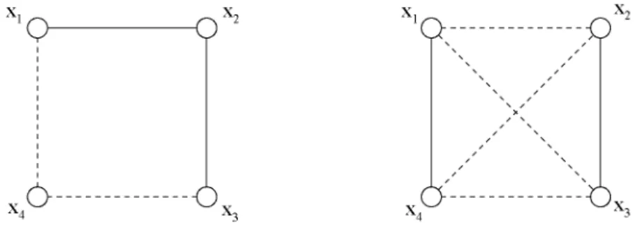
5.1 Signed graphs

Nicely simple corollaries of Propositions 1 and 2 in Section 3 hold for signed graphs, originally introduced by Harary [22]. A signed graph or s-graph is a graph (V, E) endowed with a map

E —>• { — 1,1}, that is, an assignment of either a +1 or a —1 weight to all m edges.

In this context, a flow problem which arises as a particular case of (6) is

x' = -AWATx (47)

and k, models a flow in which the adjacent agents i, k tend to increase the difference between Xi and Xk, since the flow from i to k now equals Xk — Xi (instead of x¿ — Xk, as in 2.2.1). This means that the cooperative assumption implicit in the choice of positive weights is replaced by a competitive one, the latter being described by negative weights. Such pairs of actors are sometimes called antagonistic or contrarians (see e.g. [3, 23, 33, 45]).

Contrary to the results known for (7) (or (47), with positive diagonal W), in which equilibria define a line (provided that the network is connected), the presence of negative weights may now result in higher dimensional equilibrium sets, as discussed in Section 3. The cases in which this may happen are compiled in the first item of Corollary 1 below. Minimal rank deficiencies can be also easily characterized in some cases. Since all weights are + 1 or —1, we may now define a spanning tree as positive or negative simply if its weight product is + 1 or —1, respectively, or, equivalently, if it contains an even (resp. odd) number of edges with negative weight.

Corollary 1. Let the dynamical system (47) be defined on a connected signed digraph. Then the following assertions hold.

1. The dimension of the equilibrium set is higher than one if and only if the numbers of positive and negative spanning trees coincide.

2. Provided that the requirement in item 1 holds, this dimension is exactly two if any one of the following conditions are met:

(a) There exists an edge such that the numbers of positive and negative trees including that edge are not the same.

(b) There exists an edge such that the numbers of positive and negative trees not including that edge are not the same.

(c) The signed graph has one negative weight (or one positive weight).

These results follow immediately from Propositions 1 and 2. Indeed, for the sum of weight products to vanish in a signed graph, the amount of positive trees (which are responsible for a + 1 term in the sum) must obviously match the number of negative trees (yielding a —1 in the sum). The other assertions are checked analogously in light of Proposition 2.

Simple examples illustrating the results above can be defined using the graphs shown in Figure 1. The first case, on the left of the figure, is simply a 4-cycle with two positive signs (continuous lines) and two negative signs (dashed lines). This graph has just four spanning trees, two of which are positive and the other two negative. The second example, on the right, depicts a complete graph K4 with two positive and four negative signs. According to Cayley's formula this graph has 42 = 16 spanning trees and, as detailed later, exactly half of

them are positive. This means that the dynamical system (47) should exhibit in both cases a linear manifold of equilibria with dimension greater than one.

Figure 1: Sign assignments yielding degenerate flow dynamics on (a) a 4-cycle; (b) K±. Edges with a negative sign are dashed.

In the first case, the remarks above concerning cycles Cn with even n predict a minimal rank deficiency, that is, the dimension of the equilibrium set should be two in this example. To check that in practice, we number and orientate each edge beginning on the top and according to a clockwise orientation of the cycle. Letting W = diag ( 1 , 1 , - 1 , - 1 ) , the right-hand side of (47) reads in this

-AWA* (

\

0 1 0 1

1 - 2

1 0

0 1 0 - 1

- l \ 0 - 1

2

The kernel of this matrix defines the equilibrium set and is defined by the relations

X2 — ^£4 —

Xi + £3

hence defining a two-dimensional linear manifold (a plane) of equilibria, as expected. Notice that these equilibrium points arise from a constant flow Xi — Xi+\ (i = 1 , . . . ,4, with the terminological abuse x$ = x\) which annihilates all derivatives x^, flowing in the clockwise (resp. counterclockwise) direction if x\ > X3 (resp. if x\ < X3). The equilibrium plane includes the line X\ — X2 — X3 — X4 for which the flow vanishes.

The example on the right of Figure 1 is aimed at illustrating that a higher (> 2) dimen-sional equilibrium set may actually occur. The 42 = 16 spanning trees of this signed graph

the other eight are positive; the dimension of the equilibrium set must therefore be greater than one. Moreover, one can check that the trees families arising in items (a) and (b) of Corollary 1 also have exactly the same number of positive and negative trees for any choice of an edge. In this direction, note first that Kn has 2nn~3 trees including a given edge, as a consequence of the homogeneity of Kn; indeed, in the whole set of spanning trees a total amount of n(n — l)/2 edges are distributed uniformly among nn~2 spanning trees, each one including n — 1 edges. This means that any fixed edge belongs to

(n — l)nn~2

—, rr~ = 2nn~3

n(n- l)/2

spanning trees, as claimed. It follows that there are (n — 2)nn~3 spanning trees not including a given edge. For the case n = 4 both numbers are 2 - 4 = 8.

By the symmetric sign assignment, we cover all possible cases just by choosing a positive edge and a negative edge. If we fix e.g. the positive edge on the left of the figure, the set of spanning trees including that edge are those in the first row of Figure 2, whereas the second row depicts the trees not including that edge. It is a trivial matter to check that both rows include four positive and four negative trees, ruling out (for positive edges) the hypotheses arising in items (a) and (b) of Corollary 1. The same holds for negative edges (e.g. focusing on spanning trees including the edge on the top, the trees 1, 14, 15 and 16 are negative whereas numbers 5, 6, 9 and 10 are positive).

Q - P 0

ó ó O O D O p p ó o p p O Ó -O p O O -o p -o o O P

D o

o~ a p o~ P o~ P a p a P a o o~ P a o a-o a- o--o a--o -o -o o--o o -o

Figure 2: Spanning trees of the signed-iCi example.

To compute the actual dimension of the equilibrium set we define the numbering and orientation of the edges by the sequence ((1, 2), (2, 3), (3, 4), (4,1), (1, 3), (2, 4)), which yields, with weights W = diag (—1,1, —1,1, —1, —1),

/ 1 - 1 - 1 l \ •1 1 1 - 1 •1 1 1 - 1 1 - 1 - 1 1

-AWAT

\

J

Now the equilibrium set is three-dimensional, being defined by the identity

so that in this case the rank drop in the product AWAT (and the dimension of the equilibrium set) is indeed greater t h a n two. Note that, again, these equilibrium solutions yield non-vanishing flows in the graph edges, except for those in the line X\ — X2 — 3?3 — X4.

5.2 C a s e of s t u d y : a sinusoidal flowrate

Driving the attention to the results in Section 4 let us assume t h a t , in the setting of Theorem 1, the nonlinear flowrate in the first edge takes the form

,A(Ci,/x) = u; + /xsin(Ci), (49) where a; is a fixed real constant. Note t h a t the form assumed for f\ equals the one arising

in Kuramoto models of coupled oscillators, as discussed in subsection 2.2.2. The weight in the first edge will capture not only the bifurcation parameter ¡1 but also the nonlinearity, according to (29), which yields in this case

W1( C i ^ ) = /xcos(Ci). (50)

The remaining edges are assumed to satisfy the requirements (b) and (c) in subsection 4.1, with flowrates given by (28).

The specific form of the nonlinear flowrate (49) makes it possible to guarantee the ex-istence of a bifurcating equilibrium for this flow network, by using a Lyapunov-Schmidt reduction. To simplify the discussion we will assume for the moment that the first edge (namely, the one accommodating the nonlinear flow) is not a bridge and, without loss of generality, we work in the invariant hyperplane defined by k* = 0, in the notation of Lemma 3 and Theorem 1. With the splitting shown in (22), the dynamics on this hyperplane (cf. (34)) reads as

y' = -ÁIf1(<:uti)-ÁIWÁ^Ey. (51)

Note t h a t (1 stands for the product A]Ey; this, together with equation (23), allows us to write the equilibrium conditions for (51) as —ATfi(AjEy,¡JL) + WiATAj Ey — ATWAjEy = 0 and, using Lemma 2, we split this condition in two, namely

h{Á¡Ey^) = W1ÁjEy (52a)

ATWÁ¡Ey = 0. (52b)

The former is simply the scalar equation

LV + /ism((l) = Wl(l. (53)

Note t h a t the bifurcation condition stated in the first item of Theorem 1 fixes the value of W\ = ficos(d) < 0; from elementary calculus we then conclude that the unique solution to

in (—7r/2,7r/2) yields a singular equilibrium (CÍ, /-**)• The remaining equilibrium components can be derived in a Lyapunov-Schmidt fashion from the second equation in (52), restated as

W^ÁjEy + ÁYWÁjEy = 0. (55)

We use the fact that ATWAj is nonsingular provided that the first edge is not a bridge, since

Ar has in this case full row rank and W is positive definite. The remaining components of the equilibrium Ey will come from the splitting

Ey = (AAj)-\AAj)Ey = (AVA])-\ÁVÁ] Ey + AÁjEy). (56)

Indeed, inserting this splitting into the second term of the left-hand side of (55) we get the component (AYA^)~1AYA^Ey in terms of (\ = AjEy. The example in subsection 5.3 illustrates this idea in a simpler setting.

The discussion above guarantees that a singular equilibrium indeed exists for the flow network with nonlinearity given by (49). Conditions guaranteeing that a saddle-node bifur-cation actually occurs come from Theorem 1, according to which it is enough to check the transversality conditions in (31). In our framework these are easily seen to amount to

^ O ^ s i n ( G ) . (57)

In light of (54), it is a trivial matter to check that both conditions hold provided that u ^ 0; under this assumption a saddle-node bifurcation necessarily exists. The example discussed in subsection 5.3 will be of help in order to illustrate this analysis.

Note finally that if the edge accommodating the nonlinear flowrate is a bridge, things get simpler. This is in particular the two-oscillators case considered in [16] (cf. Section 3.2 there), where a saddle-node bifurcation is reported for the parameter value ¡i = —u, with cos((i) = 0 (fi and u standing for ciu and u\, respectively, in the notation of [16]; the identity

¡i = —u follows from the condition n = 1 there). The results reported in [16] can be seen

as a particular instance of the phenomenon predicted by our previous analysis; specifically, their ad hoc conditions are now better understood in the light of Theorem 1 above: indeed, if the first edge is a bridge then it necessarily belongs to all network spanning trees, and the first item in Theorem 1 then yields W\ = 0. In light of (50) this necessarily means that either ¡i or cos((i) are null, but the vanishing of the former is ruled out by the conditions (57) emanating from the second item in Theorem 1. The condition sin(£i) = 1 then follows (mind the angle convention in [16]), and the bifurcation value ¡i = —u is finally derived in our approach by setting W\ = 0 in (53).

5.3 An example on a 3-cycle

Assume t h a t the first edge is directed from nodes 1 to 2 and accommodates a nonlinear flow defined by the flowrate depicted in (49), whereas edges 2 and 3 are directed from node 2 to node 3 and from node 3 to node 1, respectively, with the flowrates in those edges given by W2(x2 — X3) and W3(X3 — x\), both W2, W3 being positive.

System (27) reads as

x\ = —u — ¡1 sin(xi — X2) + W3(x3 — X\) (58a)

x'2 = UJ + fj,sm(x\ — X2) — W2(x2 — X3) (58b)

x'3 = W2(x2 - X3) - W3(x3 - xi) (58c)

whereas, taking k* = 0, the reduction (34) is

y[ = -uj-/ism(yl - y2) + W/ 3(-2y1 - y2) (59a)

y'2 = u + fjL sin(yi - y2) - W2(yi + 2y2). (59b)

To make computations as simple as possible we further fix W2 = W3 = 1. Note t h a t the determinantal expansion (19) yields, in a 3-cycle, the sum of products W1W2 + W1W3 + W2W3 and the critical value arising in item 1 of Theorem 1 (cf. (30)) is

W2W3 Wi =

W2 + W3

and therefore Wx = - 1 / 2 if W2 = W3 = 1.

With W2 = W3 = 1, equilibria of (59) are easily checked to satisfy the linear restriction V\ + 2/2 = 0, which makes it possible to write the scalar nonlinear equation (53) as

u + tism(2y1)+y1 = 0. (60)

The singular solutions for this scalar equation correspond to the critical value

W1=ficos(2y1) = -l/2. (61)

From (60) and (61) one easily gets the j/i-component of the singular equilibrium from (54), t h a t is,

tan(2y1) = 2(o; + y1). (62)

For any w G R , this equation has a unique solution y\ with 2y\ G (—ir/2,7r/2), which can be only written explicitly if u = 0 (in this case, and only in this case, y\ = 0). For any u, the bifurcation value can be written in terms of y\ simply as

¡j* = ^-—. (63)

P 2cos(2yí) v ;

Finally, the other component of the singular equilibrium solution is just y2 =

using the scalar reduction (60), arguments from elementary calculus (which we omit for the sake of brevity) show that a pair of equilibrium solutions do exist for ¡i less t h a n (and close enough to) //*, the latter given in (63), whereas no solution is locally displayed if ¡i > ¡i* (and always in a neighborhood of ¡i*). By contrast, if u = 0 the failing of the second condition in (57) at the origin rules out a saddle-node bifurcation but yields in this case a pitchfork bifurcation; note, indeed, that y\ = 0 is always a solution to (60) if u = 0, and that locally around ¡i* = —1/2, two additional (resp. no additional) solutions are depicted for ¡i < ¡i* (resp. ¡i > ¡i*).

5.4 O n t h e t r a n s v e r s a l i t y c o n d i t i o n ( 3 2 )

Our last example is aimed at illustrating that the transversality requirements in the saddle-node bifurcation (Theorems 1 and 2) may not be automatically met in more general settings. Specifically, we want to show that the claim in Lemma 2 (that is, the property depicted in (32)) may not be true if another weight apart from W\ becomes negative and the tree-based conditions in items (c) and (d) of Theorem 2 do not hold. To this end, consider the weighted digraph depicted in Figure 3, which is obtained after removing one edge from K±.

Figure 3: Weighted K± — {e}.

We let the edge corresponding to the NW-SE diagonal in Figure 3 be the first one, and direct it from N W to SE, and number and direct the remaining ones clockwise and beginning at the top. Some simple computations yield

/ W1 + W2 + W5 -W2

AYWAj = I -W2 W2 + W3

V -Wx -W3 Wx

By taking W2 + W3 = 0, with W2 ^ 0 ^ W3, the second column of this matrix easily shows t h a t AT = (l 0 —l) may well belong to the image of ATWAJ (so t h a t (32) is not met) even when this matrix is singular; the latter may be shown to happen e.g. if W4 + W5 = 0, since the determinant of the nodal matrix above can be easily written as

(W2 + W3)(W1W4 + W W 5 + W W 5 ) + W2W3{WA + W5). (64)

The condition Ar G imArH^4j holds here regardless of the sign of W\ and may well happen