TECHNICAL PAPER
Journal of the South african
inStitution of civil engineering
Vol 56 No 3, October 2014, Pages 77–87, Paper 1030
DR JAVIER OLIVA is a research assistant in the Department of Mechanics and Structures in the School of Civil Engineering at the Technical University of Madrid (UPM), Spain. He received his PhD from the same institute in 2011. Before joining UPM he worked as a consulting structural engineer in a private company. His research interests include structural dynamics and biomechanics. He lectures at Saint Louis University (Madrid campus), and has authored or co-authored 15 conference and scientific journal papers, and participated in several research projects with companies and administrations. Dr Oliva also collaborates with AR2V, an independent firm spesialising in the design of bridges and other structures.
Contact details:
Department of Mechanics and Structures
School of Civil Engineering, Technical University of Madrid 28040 Madrid, Spain
T: +34 91 336 5358, F: +34 91 336 5367 E: [email protected]
PROF JOSÉ M. GOICOLEA received his PhD from the University of London in 1985. Since 1993 he has been full professor in the School of Civil Engineering at the Technical University of Madrid (UPM), Spain. His research is mainly focused on structural dynamics and cardiovascular biomechanics. He has authored more than 100 conference and scientific journal papers, and has developed around 60 research projects for companies and administrations. He is Vice-President of the Spanish Society for Numerical Methods in Engineering (SEMNI), and is also a member of the General Council of the International Association for Computational Mechanics (IACM).
Contact details:
Department of Mechanics and Structures
School of Civil Engineering, Technical University of Madrid 28040 Madrid, Spain
T: +34 91 336 6761, F: +34 91 336 5367 E: [email protected]
DR PABLO ANTOLÍN is a research assistant in the Department of Mechanics and Structures in the School of Civil Engineering at the Technical University of Madrid (UPM), Spain. He received his PhD from the same institute in 2013. His research is mainly focused on structural dynamics and numerical methods, including isogeometric analysis. During his doctorate studies he taught computational mechanics in the School of Civil Engineering at UPM. He has also participated in several research projects concerning, for example, the turbulent wind effet on tall high-speed railway bridges or membrane structures. He has authored or co-authored several conference and scientific journal papers.
Contact details:
Department of Mechanics and Structures
School of Civil Engineering, Technical University of Madrid 28040 Madrid, Spain
T: +34 91 336 5358, F: +34 91 336 5367 E: [email protected]
PROF MIGUEL Á ASTIZ has more than 30 years’ experience in major bridge design. He shares his professional activity between academia, where he currently holds the Chair in Bridge Design in the School of Civil Engineering at the Technical University of Madrid (UPM), Spain, and professional practice with Carlos Fernández Casado S L, a prestigious global design firm. Prof Astiz has designed a multitude of major bridges, the River Suir cable-stayed bridge in Waterford, Ireland, being one of his most recent projects. He is President of the Spanish Scientific Association for Stuctural Concrete (ACHE).
Contact details:
Department of Mechanics and Structures
School of Civil Engineering, Technical University of Madrid 28040 Madrid, Spain
T: +34 91 336 6760, F: +34 91 336 5367 E: [email protected]
Keywords: underspanned suspension bridges, road roughness, vehicle– bridge dynamic interaction, deck vibrations, penalty method
INTRODUCTION
Structural system
In underspanned suspension bridges the ten-sioned cable system is located below the deck, and tendons are deflected by struts or braces that are connected with the girder and thus transmit the upward cable deviation forces that help to support it. Cables are anchored in the deck over abutments and piers, if piers exist. This system is more efficient in single-span or simply-supported structures; in con-tinuous bridges the under-deck cable system contribution in the negative bending regions (over piers) is very small, and tendons should be placed above the girder in those parts (Ruiz-Terán & Aparicio 2007b). This paper deals only with simply-supported bridges.
Cable forces are transferred into the deck as anchorage reactions that introduce axial compression stresses, and only verti-cal reactions appear at bearings. Cables are prestressed to neutralise permanent loads. Therefore, tendons are tensioned, the deck is compressed and bending is reduced due to the upward deviation forces in the deck.
This typology has significant advantages. In the first place, bridge cost is reduced due to the high structural efficiency. This effi-ciency in the use of materials arises from the
important contribution of the axial response compared with bending. Furthermore, because of this bending response reduction, it is possible to build more slender decks, so the advantages are not only economical, but also aesthetic. It is important to remark that, although deck height is reduced, the overall structural depth is increased due to the loca-tion of the cable system. Hence, substantial vertical clearance is required below the road for this type of bridge to be built.
Simply-supported underspanned suspen-sion viaducts can span medium distances of around 80 m that would otherwise be bridged with a multi-span solution (for example a three-span bridge with lengths 24+32+24 m and a deck height of 1.5 m). Hence this solution avoids the erection of piers, with the subsequent reduction of con-struction time and other complications. In the case of a conventional solution with one single span, the resulting structure would be much heavier. Depending on the total weight of the bridge, an underspanned suspension structure could even be lifted into place by a crane, which would significantly reduce the disturbances produced during construction. On the other hand, their inherent light-ness makes these bridges more sensitive to certain dynamic actions.
Dynamic behaviour
of underspanned
suspension road bridges
under traffic loads
J Oliva, J M Goicolea, P Antolín, M Astiz
Underspanned suspension bridges are structures with important economical and aesthetic advantages, due to their high structural efficiency. However, road bridges of this typology are still uncommon because of limited knowledge about this structural system. In particular, there remains some uncertainty over the dynamic behaviour of these bridges, due to their extreme lightness. The vibrations produced by vehicles crossing the viaduct are one of the main concerns. In this work, traffic-induced dynamic effects on this kind of viaduct are addressed by means of vehicle–bridge dynamic interaction models. A finite element method is used for the structure, and multibody dynamic models for the vehicles, while interaction is represented by means of the penalty method. Road roughness is included in this model in such a way that the fact that profiles under left and right tyres are different, but not independent, is taken into account. In addition, free software (PRPgenerator) to generate these profiles is presented in this paper.
Background
First examples of bridges with the tensioned system located below the girder are found in the nineteenth century. In the 1830s G H Dufour built the Ile aux Barques Bridge in Geneva, Switzerland, with a main span of 33.5 m (Peters 1987), and J Smith erected the Micklewood Bridge (Figure 1), a 30 m single-span structure, in Scotland (Drewry 1832). In both structures the girder rests on chains that are anchored into the deck. Chains and deck are connected to each other by vertical struts that are in compression, in contrast with the vertical tensioned elements of tradi-tional suspension bridges.
In the last quarter of the twentieth century this kind of structure started to reappear. Some authors ascribe this reappearance as having been initiated by Fritz Leonhardt’s design for the Neckar Valley Bridge in the late 1970s. Leonhardt used this solution in order to avoid pier foundations in the hillside due to soil-related problems. End piers were removed in the design stage, and first and last spans are supported by cable systems located below the girder. These cables introduce vertical reactions in the deck by means of vertical elements and thus replace the eliminated piers; Figure 2 shows one of these systems. Ruiz-Terán and Aparicio (2007b) presented a wide and exhaustive state-of-the-art study of these bridges, considering the Neckar Valley viaduct as the birth of the typology (the term
under-deck cable-stayed bridges is used by
these authors), and therefore nineteenth cen-tury structures are not included in their work. Other researchers conceive these bridges as an evolution from externally prestressed bridges in which bending behaviour is enhanced by locating tendons outside cross-section bounds. These authors call these structures
bridges with highly eccentric external tendons (Mutsuyoshi et al 2010).
Examples of simply-supported unders-panned suspension bridges can be found all over the world, for instance the Tobu and Inachus footbridges in Japan, or the Truc de la Fare road bridge in France which spans 53 m. A very exhaustive review can be found in Ruiz-Terán and Aparicio (2007b), and several examples of footbridges are explained in Strasky (2005).
In spite of the important advantages pointed out above, underspanned suspen-sion bridges are still unusual structures, and authorities remain reluctant to build them. This is due to limited knowledge about these viaducts. One of the first concerns is the shear capacity, as the girder depth is
substantially reduced, but it has been proved experimentally that the shear resistance is even higher than in conventional girders (Mutsuyoshi et al 2010). The structural behaviour of this kind of bridge was studied both analytically and experimentally in Witchukreangkrai et al (2000), Aravinthan
et al (2001), and Ruiz-Terán and Aparicio
(2007a). Some design criteria were proposed by Ruiz-Terán and Aparicio (2008) by using simply-supported 80 m span bridges.
Nowadays one of the main concerns is the lack of knowledge regarding the dynamic response of these bridges to different excita-tions. Ruiz-Terán and Aparicio (2009) dealt with the sudden breakage of stay cables due to a truck impacting with them, which was the principal reason why this solution for the
Figure 1 Micklewood Bridge (adapted from Drewry 1932)
Figure 2 Sketch of Neckar Valley Bridge end span
Figure 3 Vehicle model: (a) side view, (b) rear view
(a) Side view (b) Rear view
Y
yb γb
1.56 m 3.17 m
4.73 m 5.00 m
cs1,cs2 cs3,cs4
yfa
yra
ct1,ct2
ks1,ks2
kt1,kt2
ks3,ks4
kt3,kt4
X
yd
αb
αra,αfa
cs1,cs3 ks1,ks3 cs2,cs4 ks2,ks4
ct1,ct3
0.50 mcd kd
2.05 m
kt2,kt4 ct2,ct4
0.32 m 0.32 m
ct3,ct4 kt1,kt3
0.705 m
Kirchheim overpass in Germany, designed by Jörg Schlaich, was rejected in 1987.
Another important issue is the vibrations induced by the crossing of vehicles over the bridge. The reduction in girder depth leads to high traffic-induced accelerations. According to Ruiz-Terán and Aparicio (2010), the depth of the deck in road bridges of this kind, with short and medium spans, is governed by the serviceability limit state of vibrations. The same happens in pedestrian bridges (Tsunomoto & Ohnuma 2002). Muttoni (2002) studied the live load effects on this kind of road bridge by using static models. Ruiz-Terán and Aparicio also studied this issue in two papers (2007a; 2008) – in the 2007a study live load effects were considered by means of static models, while in the 2008 study dynamic analysis was performed with 400 kN vehicles crossing the bridge at 60 km/h (trucks were modelled as moving loads, so no dynamic interaction was taken into account).
Research aim and limitations
In this work, the dynamic response of under-spanned suspension bridges under the action
of running vehicles is analysed by means of a vehicle–bridge interaction (VBI) model. Road roughness is considered in the simulations, and differences between excitations under left and right tyres are taken into account by means of an approach presented by the authors in Oliva et al (2013a; 2013b).
The main objective of this work is to shed some light on the dynamic behaviour of these viaducts under traffic loads, as this knowledge is still limited. Important traffic-induced dynamic excitation will happen due to the extreme lightness and flexibility of this struc-tural solution. In fact, accelerations in these decks are higher than in conventional bridges.
In this study one bridge of medium length is employed as a representative exam-ple, and only one set of support conditions is considered. Double bearings are set at both abutments, and therefore torsional rotation is prevented at those points. The use of sliding supports will not have a significant influence on the results, as vertical and torsional modes will not be affected. Another solution could be the use of only one support at one abutment. Structural torsional stiff-ness would decrease significantly and hence
torsional frequencies of vibration would also be reduced. However, the low torsional rigid-ity inherent in this structural system makes this option inadvisable, and hence this solu-tion is not considered in this work.
VEHICLE–BRIDGE
INTERACTION MODELS
Vehicle
A two-axle truck is considered in this work. This vehicle model has also been used by other authors, e. g. Law and Li (2010), and is based on the H20-44 truck design loadings included in the AASHTO (1998) specifica-tions. In this study a seat is added to the truck model in order to assess the dynamic effects on the driver.
The complete model consists of three rigid bodies that represent the box and both axles, plus one DOF mass that reproduces the driver seat. The vehicle model and its eight DOFs are depicted in Figure 3. The driver seat mass (md = 80 kg) is con-nected to the vehicle body by a vertical spring (kd = 10 507 N/m) and dashpot (cd = 876 N· s/m). Driver seat properties are taken from Zuo and Nayfeh (2007). Truck model mechanical properties can be found in Zhu and Law (2002).
Structure
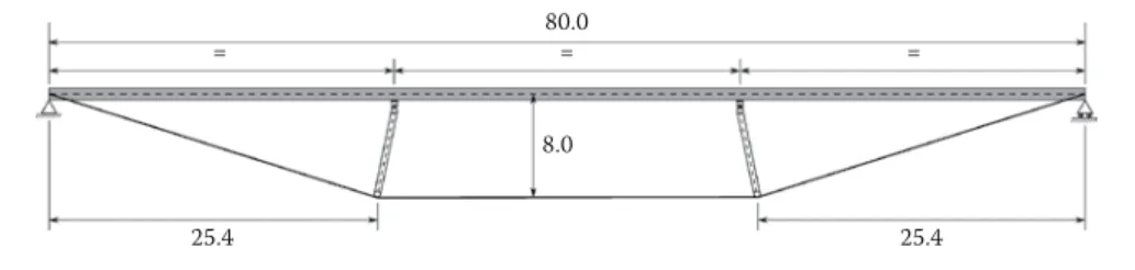
An 80 m long simply-supported under-spanned suspension viaduct is considered in this work (Figure 4), as described in Ruiz-Terán and Aparicio (2009). The cable system is anchored in the deck over the two abut-ments and is deflected by two slightly inclined steel struts. The deck is a voided concrete girder with a depth of 1 m and a total width of 13.2 m (Figure 5). Double supports are set at both abutments, hence torsional rotation is not permitted at those points.
This bridge is modelled by means of the finite element method – shells are employed to represent the deck and beams for the struts, and both kinds of elements consider shear deformation and adopt reduced inte-gration. Cables are represented by means of truss elements. Forces and displacements induced in the bridge by the crossing vehicles are small enough to adopt linear elastic behaviour in the structure. Nonstructural masses representing other dead loads, such as pavement and safety walls, are included in the model. The damping matrix is built following the Rayleigh method by setting a damping ratio of 1% for the first mode (0.78 Hz) and also for 50.0 Hz. Figure 6 shows the first bending mode of vibration (1st global mode) and the first torsion mode
of vibration (3rd global mode).
Figure 4 Sketch of bridge and main dimensions (m)
25.4 25.4
80.0
8.0
= = =
Figure 5 Bridge cross-section sketch, dimensions in metres (voids are filled over struts and on abutments)
13.2
0.40 0.17
0.25
3.0
1.0
3.0
7.2
Figure 6 Bridge first bending and torsion modes: (a) 1st bending mode (f
1 = 0.78 Hz), (b) 1st torsion mode (f
Vehicle–bridge dynamic interaction
Vehicle–bridge vertical interaction is gathered through a node-to-surface contact at each vehicle tyre, and those contacts are imple-mented by means of the penalty method. This method does not introduce additional vari-ables to the problem, and the computation is therefore faster. On the other hand, the con-straint equation is only fulfilled approximately and some penetration will be unavoidable. This penetration will depend on the penalty parameter ε. When there is no contact, no forces are added and separation is reproduced in the numerical model. The whole system is set out as a fully coupled system of equations and it is solved by direct time integration with the HHT-α method (Hilber et al 1977). This methodology has two main advantages over other fully coupled methods (Deng & Cai 2010; Yin et al 2010; Neves et al 2012): (1) modal superposition is not used for the bridge subsystem and hence structural non-linearities could be considered, and (2) vehicle tyres can lose contact with the deck surface. This separation capability is of interest in certain situations, as will be shown below.As stated before, the constraint equation is fulfilled approximately when the penalty method is employed. Hence the solution is only an approximation of the correct enforce-ment of the constraint condition obtained with the Lagrange multiplier method (Wriggers 2002). In Figure 7(a) penetration at the right rear wheel when the vehicle crosses the bridge at 110 km/h is shown when Penalty and Lagrange multiplier methods are employed; road roughness is included. As can be seen, some penetration takes place with the penalty method. However, the contact force is the same in both cases. Figure 7(b) shows the vertical reaction under the same wheel during a short period of time, in order to facilitate visualisation. It can be concluded that the penalty method leads to correct results, although some penetration is inevitable.
ROAD SURFACE DESCRIPTION
Road roughness is generally the most important source of dynamic excitation in road traffic, hence a correct definition of the road surface is a key point in vehi-cle–bridge interaction problems. When the actual profile of a particular road stretch is not needed, but a set of profiles that are representative of a certain sort of road, stochastic definitions for the generation of synthetic profiles have to be used, as for example in Deng and Cai (2010). The fact that profiles under left and right tyres are different, but not independent, is seldom considered in this kind of simulation; therefore it is assumed that the road profile is constant across the deck width. In this paper those differences are considered by means of a procedure developed by the authors and described in Oliva et al (2013a). The influence of left–right dissimilarity on road vehicle–bridge interaction dynamics has been shown in Oliva et al (2013b).In order to facilitate the generation and use of parallel profiles for other researchers,
the authors have implemented a free-to-download program (http://w3.mecanica.upm. es/prpgenerator/index.php) that creates pairs of profiles with the mentioned procedure. This simple application named PRPgenerator was developed in MATLAB© and it is
intro-duced for the first time in this paper. A brief description can be found in Appendix A.
The procedure employed in this work for considering that fact assumes hypotheses of road surface isotropy and homogene-ity. In a homogeneous and isotropic road surface every straight profile has the same statistical characteristics, independent of its direction or position. Thus, parallel profiles along the road share statistical properties, but are not the same. Given that, the cross-Power Spectral Density (Gx) of the pair of parallel profiles at a certain distance is obtained from the direct Power Spectral Density or PSD (G). The methodology is not explained here, for the sake of briefness, but it is detailed in Oliva et al (2013a; 2013b). The ISO-8608 (1995) PSD definition must be slightly modified in order to fulfil the
Figure 7 Penalty method versus Lagrange multiplier method: (a) penetration at right rear wheel, (b) contact force at right rear wheel
10
Pe
ne
tr
at
io
n (μ
m
)
8
6
4
2
0
Time (s)
5 4
3 2
1 0
Lagrange multiplier Penalty (ε = 108)
Fo
rce
(k
N
)
70 68 66 64 62 60 58 56 54 52
3.5 3.4
3.3 3.2
3.1 3.0
Time (s)
Lagrange multiplier Penalty (ε = 108)
(a) Penetration at right rear wheel (b) Contact force at right rear wheel
Figure 8 Parallel road profiles at 2.05 m
El
ev
at
io
n (m
m
)
20
–20 –15 –10 –5 0 5 10 15
180 160 140 120 100 80
60 40 20 0
Distance (m)
isotropy admissibility conditions (Kamash & Robson 1977). It must be set constant and equal to G(na) at all wave numbers below a limiting wave number na. Thus it becomes acceptable, as its integral is bounded and the function remains monotonically non-increasing. This limit is set as na = 0.01 m-1,
which is the minimum spatial frequency considered in roads (ISO-8608 1995). The PSD becomes:
G(n) =
ìïï
ïï
íï
ïïïî
G(n0) æ
ç
ènna0æç
è–2
for n ≤ na
(1) G(n0)æ
ç
ènn0
æ
ç
è–2
for n > na
where G(n) is the one-sided power spectral density for the spatial frequency or wave number n and G(n0) is the one-sided power spectral density for the reference spatial frequency n0 = 0.1 m-1. The value for G(n
0) is
prescribed by ISO-8608 (1995) as a function of the road class.
Two parallel road profiles are generated as follows (Sayers 1998):
y1(x) =
∑
Ni√
2G(ni)∆n cos(2πnix + φi) (2)y2(x) =
∑
Ni æç
è√
2G(ni)∆n cos(2πnix + φi)+
√
2(G(ni) – Gx(ni))∆n cos(2πnix + θi)æç
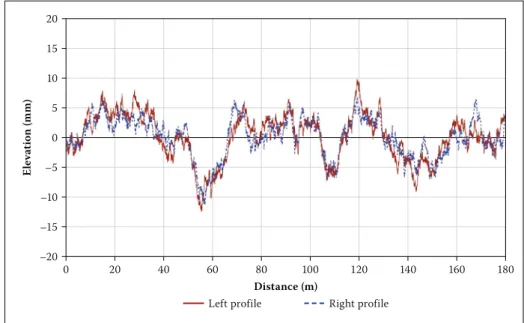
è (3)where φi and θi are two sets of random phase angles which are uniformly distributed from 0 to 2π. An example of two class A parallel profiles is depicted in Figure 8.
NUMERICAL STUDIES
For the truck and bridge presented in this section numerical simulations are used. Geometric nonlinearities can easily be considered in the proposed framework, but nonlinear effects in the considered scenarios have been shown to be negligible. Therefore, linear models are employed in this work because of the shorter computation time required. Six different running speeds were employed (30, 50, 60, 80, 110 and 120 km/h) in order to consider typical urban and highway vehicle speeds in different countries around the world. The road surface is assumed to be very good (class A, G(n0) = 16·10-6 m3)
(ISO-8608 1995), 2000 spatial frequencies between 0.01 m-1 and 10.0 m-1 are used in the
profile generation, and road irregularities are sampled every 2 cm in the longitudinal direc-tion. Ten road surfaces (A01, A02, ..., A10) are generated so that the results are statistically significant. Thus, 60 different simulations had to be performed for this part of the work (6 speeds x 10 profiles). The H20-44 vehicle crosses the structure in the right lane with its right wheels at a distance of 2.55 m from the right edge of the bridge (see Figure 9). Driving
on the right-hand side of the road is assumed in this work as it is the most common option in the world. The outcome of the study with left-hand traffic would be the same.
Results are obtained at every node on the bridge surface. These nodes are gathered in longitudinal lines whose transversal position and name are shown in Figure 9. The bridge surface is discretised with 14 elements in width and 81 elements in length, so that there are 15 longitudinal lines with 82 nodes per line.
With regard to the Serviceability Limit State of vibration in road bridges, Eurocode EN1990 (EN1990:2002/A1+AC 2010) is very vague, and no indication is given with respect to the comfort of passengers or pedestrians. With respect to footbridges it is stated that pedestrian comfort criteria for serviceability should be defined in terms of maximum acceptable acceleration of any part of the deck. The recommended maximum value for verti-cal acceleration is set as 0.7 m/s2. This limit is
adopted in this work as a limitation to pedes-trian comfort on the sidewalks of road bridges.
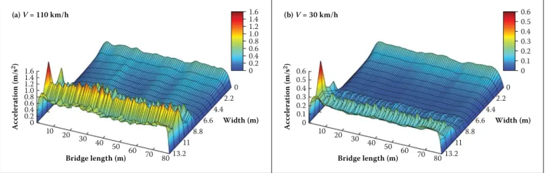
Maximum acceleration at every bridge surface node is obtained with the ten different road surfaces considered (A01, ..., A10). The mean value of those ten maxima is computed in order to get representative accelerations of the road class, instead of an absolute maxi-mum that would represent a critical situation. Figure 10 shows the mean value of maximum vertical acceleration on the whole bridge surface for vehicle speeds of 110 km/h and 30 km/h. In both cases high accelerations are found right under the vehicle path due to local vibrations. At high speeds these accelerations are significantly higher than those of the rest of the surface. At low speeds the local apexes are not so markedly protruding. Clear peaks can be noticed in the two cases near the first abutment, located precisely under the truck (between lines A7 and V4); the maximum value is in line V4, because it belongs to the cross-sectional cantilever. These first abut-ment high values are caused by the sudden entrance of the vehicle. Vertical acceleration
Figure 9 Vehicle transverse position and longitudinal lines (dimensions in m)
2.55 2.05 8.60
V6 V5 V4 A9 A8 A7 A6 A5 A4 A3 A2 A1 V3 V2 V1
Figure 10 Maximum vertical acceleration on the bridge surface: (a) V = 110 km/h, (b) V = 30 km/h
A
cc
el
er
at
io
n (
m
/s
2) 1.6
1.4 1.2 1.0 0.8 0.6 0.4 0.2 0
10 20 30 40
50 60
70 80 13.2 11
0 2.2 4.4 6.6 8.8
Bridge length (m)
Width (m) 1.6 1.4 1.2 1.0 0.8 0.6 0.4 0.2 0
A
cc
el
er
at
io
n (
m
/s
2) 0.6
0.5 0.4 0.3 0.2 0.1 0
10 20 30 40
50 60
70 80 13.2 11
0 2.2 4.4 6.6 8.8
Bridge length (m)
Width (m) 0.6 0.5 0.4 0.3 0.2 0.1 0
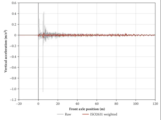
of the node located in line V4 at 1.0 m from the abutment, with V = 50 km/h and surface A01, is depicted in Figure 11 by the label Raw; high accelerations appear when each truck axle enters the bridge.
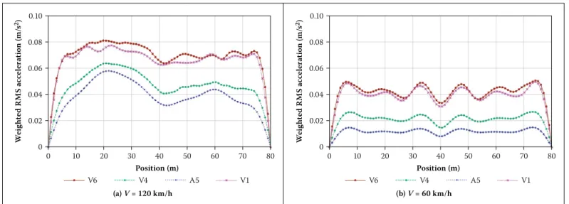
In Figure 12 maximum acceleration of some significant lines (V1, V4, V6 and A5) is depicted for 120 and 60 km/h. A peak at the beginning of V4 is easily noticable in both cases. For 120 km/h accelerations in nodes belonging to V4 are clearly the highest in the bridge, for 60 km/h local vibrations are less important and V4 accelerations are similar to those found in lines V1 and V6. Acceleration in the bridge longitudinal midline (A5) is always significantly lower than in the canti-levers, which fact indicates the relevance of torsion effects.
The Eurocode EN1990 limitation is generally fulfilled at 60 km/h, and is only
violated near the first abutment because of the very local effects of the vehicle entrance, as explained before. At high speed (120 km/h) the maximum acceleration crite-rion is not satisfied in the vehicle side canti-lever (V4–V6) all along the bridge length. It is remarkable that vertical acceleration along the bridge length is uniform for every vehicle speed, with the exception of the vehicle entrance region.
Two different standpoints exist regarding the acceleration effects on human comfort. The first considers that people are affected most by the largest peaks, and therefore maximum acceleration is limited as in Eurocode EN1990. According to the second school of thought it is assumed that the degree to which vibration may be noticed or tolerated is determined by some averaged effect over a period of time. International
standard ISO-2631-1 (1997) specifies a meth-od of evaluation of the effect of vibration on human beings by means of the weighted root-mean-square (RMS) acceleration which is defined as:
aw = 1
T
∫
T
0 aw2(t)dt (4)
where aw(t) is the weighted acceleration as a function of time and T is the duration of the vibration.
Human response to vibration is a function of frequency and therefore data must be weighted in order to give greater prominence to frequencies where humans are most sensitive. Analogue transfer functions that determine the frequency weighting are speci-fied in ISO-2631-1 (1997). Those functions are transformed into digital filters by means of bilinear transformations.
For a standing person subjected to verti-cal accelerations underneath their feet, as is the case with a pedestrian on a bridge, Wk weighting is applicable. Its parameters are given in ISO-2631-1 (1997). As an example, Figure 1 shows vertical weighted acceleration (aw(t)) in line V4 at 1.0 m from the first abut-ment; high-frequency peaks are eliminated by the frequency weighting. Reaction to vibration depends on many factors (frequency, duration of vibration, activity, age, etc), and therefore absolute limits cannot be established, only indications of likely human reactions. Some limits are given by the Department of Environment and Conservation of New South Wales in Australia (DEC 2006), but no specific values are provided for bridges. The highest admissible value in buildings is set as 0.08 m/s2. A weighted RMS acceleration of
0.08 m/s2 is also adopted in British Standard
BS 6472:1992 (1992) as a value below which there exists a low probability of adverse comment from users of residential buildings
Figure 11 Raw and weighted vertical acceleration in line V4 at 1.0 m from the first abutment,
V = 50 km/h
Ve
rt
ic
al a
cc
el
er
at
io
n (
m
/s
2)
–0.6
–0.8
–1.0
–1.2 –0.4 –0.2 0 0.2 0.4 0.6
–20 0 20 40 60 80 100 120
Front axle position (m) ISO2631 weighted Raw
Figure 12 Maximum vertical acceleration on representative longitudinal lines: (a) V = 120 km/h, (b) V = 60 km/h
A
cc
el
er
at
io
n (
m
/s
2)
1.8 1.6 1.4 1.2 1.0 0.8 0.6 0.4 0.2 0
A
cc
el
er
at
io
n (
m
/s
2)
1.8 1.6 1.4 1.2 1.0 0.8 0.6 0.4 0.2 0
Position (m)
80 70 60 50 40 30 20 10 0
Position (m)
80 70 60 50 40 30 20 10 0 0.7 m/s2
V6 V4 A5 V1 V6 V4 A5 V1
(a) V = 120 km/h (b) V = 60 km/h
during the day, with a time of exposure to vibration lower than 225 seconds (the bridge in this study is crossed by a person in approxi-mately one minute). Building limits are not directly applicable to bridges. The same value (0.08 m/s2) is defined in the German guideline
VDI 2057 (2002) as a limit above which vibra-tion is strongly perceptible by a human being. Higher values would probably be tolerated by pedestrians on a road bridge, but it seems reasonable to adopt 0.08 m/s2 as a guidance
value for human comfort on viaduct decks, although presumably conservative.
As for maximum acceleration, weighted RMS acceleration is computed for every bridge surface node with the ten different road surfaces considered, and the mean value is calculated. Figure 13 shows the mean value of the weighted RMS acceleration all over the bridge surface. First the abutment peaks and high values on the vehicle trajectory disappear, and the highest values are now obtained in the bridge edges (V1 and V6), both with high and low speeds. In Figure 14, values in some significant lines (V1, V4, V6 and A5) are depicted for 120 and 60 km/h.
Weighted RMS remains at acceptable lev-els on the whole deck surface for all vehicle speeds. It is remarkable that differences
between the left and right bridge edges, which were evident when using maximum acceleration values, almost vanish if weight-ed RMS is employweight-ed.
With respect to the Dynamic
Amplification Factor (DAF) of vertical dis-placement, the mean value of the ten cases is depicted in Figure 15 for the bridge midline (A5) considering different vehicle speeds.
High DAFy values appear and they are highly influenced by vehicle speed. DAF values as high as 1.54 are reached with V = 120 km/h near the first strut. These high values indi-cate the huge relevance of dynamic effects on this kind of structure.
Regarding vehicle vibration, Figure 16 shows vertical acceleration at the driver seat when the vehicle runs at 120 km/h with
Figure 13 Weighted RMS vertical acceleration on the bridge surface: (a) V = 110 km/h, (b) V = 30 km/h
W
ei
gh
ed R
M
S a
cc
el
er
at
io
n (
m
/s
2)
0.10 0.08 0.06 0.04 0.02 0
10 20 30 40
50 60 70 80 13.211
4.4 6.6 8.8
Bridge length (m)
Width (m) 0.09 0.08 0.07 0.06 0.05 0.04 0.03 0.02 0 (a) V = 110 km/h
2.2 0
0.01
W
ei
gh
ed R
M
S a
cc
el
er
at
io
n (
m
/s
2)
0.04 0.03 0.02 0.01 0
10 20
30 40 50 60
70 80 13.211 4.4 6.6 8.8
Bridge length (m)
Width (m) 0.09 0.08 0.07 0.06 0.05 0.04 0.03 0.02 0 (b) V = 30 km/h
2.20 0.01
Figure 14 Weighted RMS vertical acceleration on representative longitudinal lines: (a) V = 120 km/h, (b) V = 60 km/h
W
ei
gh
te
d R
M
S a
cc
el
er
at
io
n (
m
/s
2) 0.10
0.08
0.06
0.04
0.02
0 W
ei
gh
te
d R
M
S a
cc
el
er
at
io
n (
m
/s
2) 0.10
0.08
0.06
0.04
0.02
0
Position (m)
80 70 60 50 40 30 20 10 0
Position (m)
80 70 60 50 40 30 20 10 0
V6 V4 A5 V1 V6 V4 A5 V1
(a) V = 120 km/h (b) V = 60 km/h
Figure 15 Displacement Dynamic Amplification Factor in Line A5
D
isp
la
cem
en
t D
A
F
1.8
1.6
1.4
1.2
1.0
0.8
0.6
0.4
0.2
0
Position (m)40 50 60 70 80
30 20
10 0
profile A07. The vertical response of the vehicle on the bridge and on a rigid road is compared under the same road surface condi-tions in order to assess the bridge flexibility influence. The results in Figure 16 show that bridge deflection has an effect on the driver seat.
For vertical vibrations on the seat surface, Wk weighting is also used (ISO-2631-1 1997). Figure 17 shows the mean value of weighted RMS acceleration on the driver seat consid-ering the ten surfaces – results on the bridge and on a rigid road are compared. The incre-ment is very small (maximum of 4%), and it can therefore be concluded that the bridge flexibility influence on driver comfort is of no significant relevance.
Effects of pothole presence
The eventual presence of a pothole of consid-erable size is considered by adding a 50 cm long and 5 cm deep defect on road surface A01, located in the midspan and affecting both vehicle sides. Tyre contact is lost in the pothole and high reactions appear when it is regained (Figure 18). The wheel–bridge separation capabilities of the interaction model are necessary for a correct simulation of this scenario. This behaviour produces very high accelerations in the bridge surface (Figure 19); even at low speeds, higher values are beyond 6.5 m/s2 when V = 50 km/h.
Road quality influence
Profiles of different road classes (A or Very Good, B or Good, and C or Medium) are employed in order to assess road class influ-ence in the dynamic behaviour of the deck. Profiles of different road classes are related by a scale factor:
yB(x) = yA(x) [G(n0)]B
[G(n0)]A (5)
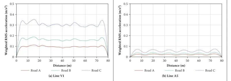
Thus B and C surfaces can be obtained by multiplying A pairs of profiles by 2 and 4 respectively. Profile A10 is employed in this section and the vehicle speed is set as 110 km/h. Maximum vertical acceleration at lines V1 and A5 is depicted in Figure 20. As can be seen, road quality has significant influence on the deck vibration, and the increase in maximum vertical acceleration is of relevance. The Eurocode limit is not reached in the midline (A5), but is exceeded in line V1 with road level B.
Road class also has influence in the weighted RMS acceleration (Figure 21) – val-ues increase when road quality declines, and exceed 0.08 m/s2 manifestly in line V1 with
road classes B and C. In the midline (A5) weighted RMS acceleration also increases, but values remain acceptable.
Figure 16 Driver seat vertical acceleration on the bridge and on the road with A07 road surface (V = 120 km/h)
Ve
rt
ic
al a
cc
el
er
at
io
n (
m
/s
2)
–1.2 –0.6 –0.8 –1.0 –0.4 0.2
0 –0.2 0.4 1.0 0.8 0.6 1.2
Front axle position (m)
0 10 20 30 40 50 60 70 80
Bridge Rigid road
Figure 17 Weighted RMS acceleration on the driver seat – bridge vs rigid road
W
ei
gh
te
d R
M
S a
cc
el
er
at
io
n (
m
/s
2)
0.14
0.12
0.10
0.08
0.06
0.04
0.02
0
120 110 100 90
80 70 50
40 30
Vertical speed (km/h) 60
Bridge Rigid road
Figure 18 Vertical reaction under left tyres with a pothole on the road (V = 50 km/h)
Re
ac
tion
(k
N
)
140
120
100
80
60
40
20
0
Front axle position (m)
50 48
46 44
42 40
38 36
1st axle == Pothole 2nd axle == Pothole
CONCLUSIONS
Vehicle-induced dynamics in under spanned suspension bridges were studied in this paper. Analyses were performed by means of a fully coupled vehicle–bridge dynamic inter-action model. The vehicle was represented
through a multibody system (MBS); the bridge was modelled with the finite element method (FEM), and interaction was gathered by means of contacts with a penalty formula-tion. The fully coupled system equations were solved by direct integration in time.
Penetration inherent in the penalty method was shown to have no effect on the relevant results against the Lagrange multiplier method, where restriction is perfectly satis-fied and no penetration takes place.
Road roughness was considered in such a way that the fact that profiles in the left and right tyres were different, but not independent, were taken into account. In order to facilitate their consideration, a parallel road profiles generation programme
(PRPgenerator) was developed by the
authors, and this is available on the web for free download as a standalone application.
A very good road class (A) was considered in the study (ISO-868 1995). Vertical accel-eration peaks appeared directly under the vehicle path due to local vibrations. Absolute maximum values arose near the first abut-ment because of sudden vehicle entrance. The Eurocode EN1990:2002/A1+AC (2010) maximum acceleration criterion was generally fulfilled on the deck surface during truck runs at urban speeds (50–60 km/h). With highway speeds (110–120 km/h) this limitation was not satisfied in the vehicle proximity, but on the rest of the deck it was. Frequency weighting
Figure 19 Deck maximum vertical acceleration with a pothole in x = 40 m (V = 50 km/h)
A
cc
el
er
at
io
n (
m
/s
2)
7
6
5
4
3
2
1
0
Position (m)
80 70
60 50
40 30
20 10
0
0.7 m/s2
V6 A5
Figure 20 Maximum acceleration with different road classes (V = 110 km/h): (a) Line V1, (b) Line A5
A
cc
el
er
at
io
n (
m
/s
2)
2.0 2.0
A
cc
el
er
at
io
n (
m
/s
2)
1.5
1.0
0.5
0
1.5
1.0
0.5
0 80
70 60 50 40 30 20 10
0 0 10 20 30 40 50 60 70 80
Distance (m) Distance (m)
0.7 m/s2 0.7 m/s2
Road A Road B Road C Road A Road B Road C
(a) Line V1 (b) Line A5
Figure 21 Weighted RMS acceleration with different road classes (V = 110 km/h): (a) Line V1, (b) Line A5
W
ei
gh
te
d R
M
S a
cc
el
er
at
io
n (
m
/s
2) 0.5 0.5
W
ei
gh
te
d R
M
S a
cc
el
er
at
io
n (
m
/s
2)
0.3
0.2
0.1
0
0.3
0.2
0.1
0 80
70 60 50 40 30 20 10
0 0 10 20 30 40 50 60 70 80
Distance (m) Distance (m)
Road A Road B Road C Road A Road B Road C
(a) Line V1 (b) Line A5
(ISO-2631-1 1997) reduced the high frequency peaks on acceleration histories, and the largest weighted RMS values were not found in the vehicle path but on both bridge edges. In addi-tion, differences between left and right viaduct edges were negligible. Weighted RMS values were low enough to be tolerated on the whole deck surface for every vehicle speed.
Significant differences were found between the bridge longitudinal midline and edges. Accelerations were clearly higher on the edges due to the excitation of the deck torsion. Therefore it would be convenient to locate sidewalks along the deck longitudinal midline, if possible, or set vehicle lanes near that line in order to reduce the excitation of this rotation.
Road class has an evident influence on pedestrian comfort. Hence, good con-struction and maintenance are of great importance in this kind of viaduct due to its dynamic sensitivity. The presence of a sig-nificant pothole could induce very high deck accelerations. Therefore, careful conserva-tion is important. With respect to vehicle behaviour, bridge flexibility causes additional vibration in the driver seat. However, the effect of the additional acceleration on driver comfort is very small – the maximum increase of the weighted RMS acceleration on the driver position was only 4%.
ACKNOWLEDGEMENTS
This work was motivated by lectures given by Dr Ana María Ruiz-Terán (Imperial
College London) at the Technical University of Madrid. The authors wish to acknowl-edge this source of inspiration. The aid of the Ministerio de Ciencia e Innovación of the Spanish government through sub-programme INNPACTO and project
VIADINTEGRA (Ref IPT-370000-2010-012)
is greatly appreciated. The authors are grateful also for support provided by the Technical University of Madrid, Spain.
APPENDIX A (
PRPgenerator
)
PRPgenerator is a simple-to-use and free
application that generates pairs of parallel road profiles. It has been implemented in Matlab© and is available as stand-alone
software. The program uses Power Spectral Density definition from ISO-8608 (1995) and assumes the homogeneity and isotropy of the road surface. PRPgenerator has been developed by the Computational Mechanics Group of the School of Civil Engineering at the Technical University of Madrid (UPM). Its theoretical background can be found in Oliva et al (2013a; 2013b), and the application is presented for the first time in this paper. It computes cross-Power Spectral Density and coherence function for parallel profiles and generates profiles with the total length, sam-ple distance and number of spatial frequencies specified by the user. Different road classes can be considered and any vehicle width may be used. Figure 22 shows the main and only window of the application.
REFERENCES
AASHTO (American Association of State Highway and Transportation Officials) 1998. LRFD Bridge design
specifications. Washington DC: AASHTO.
Aravinthan, T, Matsui, T, Hamada, Y & Shinozaki, H 2001. Structural analysis of Torisaki River Park bridge – An innovative PC bridge with large eccentric external tendons. Proceedings, 11th Symposium on
Development in Prestressed Concrete, pp 49–54.
BS 6472 1992. Guide to evaluation of human exposure
to vibration in buildings. London: British Standards
Institution.
DEC (Department of Environment and Conservation, New South Wales) 2006. Assessing vibration: A
technical guideline. Sydney, Australia: DEC.
Deng, L & Cai, C S 2010. Development of dynamic impact factor for performance evaluation of existing multi-girder concrete bridges. Engineering
Structures, 32: 21–31.
Drewry, C S 1832. A memoir on suspension bridges. London: A and R Spottiswoode.
EN 1990. 2002/A1+AC 2010. Eurocode – Basis of
structural design. Brussels: European Committee for
Standardization (CEN).
Hilber, H M, Hughes, T J R & Taylor, R L T 1977. Improved numerical dissipation for time integration algorithms in structural dynamics. Earthquake
Engineering and Structural Dynamics, 5: 283–292.
ISO-2631-1 1997. Mechanical vibration and shock – Evaluation of human exposure to whole body
vibration – Part 1: General requirements. Geneva:
International Organization for Standardization (ISO). ISO-8608 1995. Mechanical vibration – Road surface
profiles – Reporting of measured data. Geneva:
International Organization for Standardization (ISO).
Kamash, K M A & Robson, J D 1977. Implications of isotropy in random surfaces. Journal of Sound and
Vibration, 54: 131–145.
Law, S & Li, J 2010. Updating the reliability of a concrete bridge structure based on condition assessment with uncertainties. Engineering
Structures, 32(1): 286–296.
Mutsuyoshi, H, Hai, N D & Kasuga, A 2010. Recent technology of prestressed concrete bridges in Japan.
Proceedings, Joint IABSE-JSCE Conference on
Advances in Bridge Engineering-II, Amin, A F M S, Okui, Y & Bhuiyan, A R (Eds), Dhaka, Bangladesh. Muttoni, A 2002. Brücken mit vorgespannter
stahlunterspannung. Stahlbau, 71(8): 592–597. Neves, S G M, Azevedo, A F M & Calçada, R 2012. A
direct method for analyzing the vertical vehicle– structure interaction. Engineering Structures, 34: 414–420.
Oliva, J, Goicolea, J M, Astiz, M A & Antolín, P 2013a. Fully three-dimensional vehicle dynamics over rough pavement. Proceedings of the ICE – Transport, 166(3): 144-157.
Oliva, J, Goicolea, J M, Astiz, M A & Antolín, P 2013b. Relevance of a complete road surface description in vehicle–bridge interaction dynamics. Engineering
Structures, 56: 466–476.
Peters, T F 1987. Transitions in engineering – Guillaume Henri Dufour and the early 19th century cable
suspension bridges. Basel, Switzerland: Birkhäuser
Verlag.
Ruiz-Terán, A M & Aparicio, A C 2007a. Parameters governing the response of under-deck cable-stayed bridges. Canadian Journal of Civil Engineering, 34: 1016–1024.
Ruiz-Terán, A M & Aparicio, A C 2007b. Two new types of bridges: Under-deck cable-stayed bridges and combined cable-stayed bridges – The state of the art. Canadian Journal of Civil Engineering, 34: 1003–1015.
Ruiz-Terán, A M & Aparicio, A C 2008. Structural behaviour and design criteria of underdeck cable-stayed bridges and combined cable-cable-stayed bridges. Part 1: Single-span bridges. Canadian Journal of
Civil Engineering, 35: 938–950.
Ruiz-Terán, A M & Aparicio, A C 2009. Response of under-deck cable-stayed bridges to the accidental breakage of stay cables. Engineering Structures, 31: 1425–1434.
Ruiz-Terán, A M & Aparicio, A C 2010. Developments in under-deck and combined cable-stayed bridges.
Proceedings of the Institution of Civil Engineers (UK)
– Bridge Engineering, 163: 67–78.
Sayers, M W 1998. Dynamic terrain inputs to predict
structural integrity of ground vehicles. Ann Arbor,
MI: University of Michigan Transportation Research Institute.
Strasky, J 2005. Stress ribbon and cable-supported
pedestrian bridges. London: Thomas Telford.
Tsunomoto, M & Ohnuma, K 2002. Self-anchored suspended deck bridge – Pedestrian bridge of Tobu
recreation resort. National Report – Recent works on
prestressed concrete structures, Osaka, Japan: Japan Prestressed Concrete Engineering Association. VDI 2057 (2002). Human exposure to mechanical
vibrations – Whole-body vibration. Düsseldorf,
Germany: Association of German Engineers. Witchukreangkrai, E, Mutsuyoshi, H, Aravinthan, T &
Watanabe, M 2000. Analysis of the flexural behavior of externally prestressed concrete beams with large eccentricities. Transactions of the JCI (Japan
Concrete Institute), 22: 319–324.
Wriggers, P 2002. Computational contact mechanics. New York: Wiley.
Yin, X, Fang, Z, Cai, C S & Deng, L 2010. Non-stationary random vibration of bridges under vehicles with variable speed. Engineering Structures, 32: 2166–2174.
Zhu, X Q & Law, S S 2002. Dynamic load on continuous multi-lane bridge deck from moving vehicles. Journal
of Sound and Vibration, 251: 697–716.
Zuo, L & Nayfeh, S A 2007. H2 optimal control of