The effect of boundary conditions in the numerical solution of 3-D thermoelastic problems

(1)

The effect of boundary conditions in the numerical

solution of 3-D thermoelastic problems

JUAN JOSÉ ANZA and ENRIQUE ALARCÓN

INTRODUCTION

After the extensive research on the capabilities of the Boundary Integral Equation Method produced during the past years the versatility of its applications has been well founded. Maybe the years to come will see the in-depth analysis of severa) conflictive points, for example, adaptive integration, solution of the system of equations, etc. This line is clear in academic research.1-6

In this paper we comment on the incidence of the manner of imposing the boundary conditions in 3-D coupled problems. Here the effects are particularly magni-fied: in the first place by the simple model used (constant elements) and secondly by the process of solution, i.e. first a potential problem is solved and then the results are used as data for an elasticity problem. The errors add to both processes and small disturbances, unimportant in separated problems, can produce serious errors in the final results.

The specific problem we have chosen is especially inter-esting. Although more general cases (i.e. transient, 7• 8) can

be treated, here the domain integrals can be converted into boundary ones and the influence of the manner in which boundary conditions are applied will reflect the whole importance of the problem.

THE STATIONARY THERMOELASTIC PROBLEM

As is well known the general thermoelastic problem is represented by a set of coupled differential equations that have to be simultaneously solved in arder to obtain the field of temperatures and the field of stresses and strains inside the body under study.

If it is possible to assume a stationary situation the problem can be solved in two steps; in the first one a Poisson type equation

Q (J •• +-==0

'11

Ao

(1)

describes the field of temperatures. He re

fJ(x,y,

z) ==

field of temperatures

Q(x,y, z)

==

intensity of heat emission

A.

0

=

material conductivity constant

When () is obtained, the Duhamel's analogy allows the solution of the problem by solving an equivalent problem (Fig. 1 ):

(A.+

J.!)

u,· ..

+

J.IU¡ .. +X;=

o

in

n

,}l ,JJ

a;¡n¡ = l¡ in

anl

(2) U¡= U¡ in aQ2

an

=

an,

u an

2UR

when R is a set of zero measure.

t¡

Figure 1

tractions tÍ

body torces

x;·

displacements uj

stress es a j¡

equivalent tractions equivalent body torces displacements stresses

E ex

')'=

1-2v

t¡

=

rj + ')'f!n¡ X¡= Xj-')'8 ¡

u¡=

u¡ '

a¡¡= aj¡ + ')'06¡¡

As is well known the representation formula for problem (1) is:

f

a...¡;

c(x) fJ(x) + - (x, y) fJ(y) ds(y)

an

=

f

l/l(x, y):: (y) ds(y)-

f

¡J¡(x, y) V2(J dv(y)

an

1 l/l{x, y)=

-4rrr(x, y)

(3)

n

=

unit normal vector, O~ c(x) ~ 1 while that corre-sponding to problem (2) is:

c;¡(x) u;(x)

+

f

T¡;(x, y) u¡(y) ds(y)

an

·'

=

J

U¡;(x, y) t;(y) ds(y) +

J

X;U¡;(x, y) dv(y)

an

O ~ e;¡ ~ 1 i ,j

=

1 , 2, 3 and the integral kernels are defined by

1

(4)

U¡;(x,y)= [(3-4v)ó;¡+r ;r ¡]e¡

I6rrG(1-v)r(x,y) ' '

i,j= 1,2,3

T¡;(x,y)

=

-

1

2

{ar

[(l-2v)ó;¡+3r ;r

¡]}

8rr(l-v)r (x,y)

an

. .

(2)

When the volume forces are exclusively due to thermal effects it is possible to write9

-11 ( 4) as:

c;¡U¡(x)

+

f

T¡;(x, y) u¡(y) ds(y)

where

a.n

=

J

U¡;(x,y)t¡(y)ds(y)-r

J

W,¡(x,y)

a.n

ae

J

X

011 (y) ds(y)

+'Y

fJ(y) W,¡;(x, y) 11¡ ds

a.n

- rm

J

W(x, y) n¡ ds

a.n

i,j=

1,2,3

r

=

Ecx/l-2v

V2₈

_=m

W;

=

(1-2v) (1

+

v) re¡/8rrE(I-v)

e¡ being the unit vector in the coordina te direction 'i'.

THE BIEM - CONST ANT ELEMENTS

(5)

(6)

The discretisation of the previous equations as well as the geometry of the boundary domain leads to the system of equations typical of this method.4' 12 In our case we have

chosen the simplest approach, i.e. the boundary is substi-tuted by a series of N plane triangles defined by sets of three points contained on the real surface. Moreover the evolution of tractions and displacements is assumed as constant throughout every boundary element, and the values associated to a selected point inside it, for instance its centre of gravity.

The equations corresponding to problem (1) are:

N N ae(xk) c¡fJ(x¡)

+

L

Aike(xk)

=

L

Blk

-k=t k=l

an

A1k

=

J

a¡J; (x_1,y) ds(y)

an

a.nk

B1k =

f

¡J;(x1, y) ds(y)

a.nk

x1 centre of gravity of element l

l,k=1,2, ... ,N

(7)

In a problem with boundary conditions of the Dirichlet type, the coefficients of the system uf equations to be solved are the B1k type, while conversely, for Neumann conditions, they are the A type. In a Newton (or Robín) problem, there is a linear combination of both Al k and Blk,

while in a mixed problem there are sorne of the Alk type and others of the B1k type.

In a pure Neumann problem it is necessary to add one condition because the solution is undetermined. Usually this is done by fixing the value of the potential in a point and in this sense it can be said that the problem has been transformed into a mixed type one.

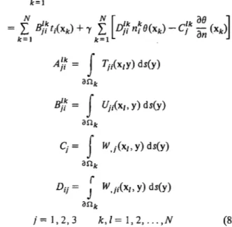
:Similarly the elastic problem can be formulated as follows:

N

c¡1u¡(x1)

+

L

AJ~

u;(xk) k=l

AJ~

=

J

T¡;(x1y) ds(y)

a.nk

BJ~

=

J

U¡¡(x1, y) ds(y)

a.nk

C¡

=

f

W,¡(x1, y) ds(y)

a.nk

r

D;¡

=

J

w,¡;(x1, y) ds(y)

a.nk

j

=

1, 2, 3 k,l=I,2, ... ,N (8)

As with the potential case it is possible to define pure problems controlled by

A

or

B

coefficients, as well as linear combinations and mixed conditions. For the same reason it is not possible to solve a problem in which all boundary conditions are defined as tractions because the displace-ments contain rigid body displacedisplace-ments. To solve this difficulty sorne convenient displacements are fixed in arder to obtain the kinematic determinacy of the body, and in this sense the problem is usually transformed into a mixed type one.

EXAMPLES

In arder to analyse the results a computer program de-scribed elsewhere9 _{was written for a UNIVAC 1108} com-puter. In aH cases material constants were chosen as:

V= 0.25

¡;.=1

ex::::! (9)

and problems selected so that a closed-fom1 solution was available to compare results.

Figure 2 shows the discretisation used to model a piece of a thick-walled cylinder submitted to an interior tempera-ture of 100° and an exterior one of 20°. Dueto the sym-metry the normal displacements in the four plane faces are zero, as well as the corresponding fluxes.

(3)

y

/ ,

1

}

IJ/ /

fJ

.1

~

1

/ 1

/y

1 .'

1 i

\ 11

1

\ 18° \ 1 /

<o/

\ 1,\,,

1 \l,\1/

1 11/

\1/

\ 1¡

\1/

X

\l¡

~--~

Figure 2

120 Temp.lnterior= 100 Temp. Exterior= 20

100

80

60

40

20 - Analytical Solution . Temperature

o~~--~2--~3~-L4--~5~~6--~7~-8~~9~-1~0~11

Radius

Figure 3

700

600

Cylinder 1 (Thermoelastic Case)

Temp. Interior = 100 Temp. Exterior= 20

500

400

300

200

- Analytical Solution

100 • Displacement

2 3 4

Figure 4

Table 1

5 6 7 8 9 10 11

Radius

Radial disp1acement Radial displacement

Radius Theoretical Comp. Radius Theoretical Comp.

4 242.07 242.61 7.5

4.5 308.72 298.20 8

5 364.27 349.98 9

6 450.66 425.13 9.5

6.5 484.28 457.26 10

7 412.77 482.46

100

60

20

-20

-60

-100

-140

2 3

-180 - Analytical Solution

-220

-260

. Normal Tension

+ Tangential Tension O Radial Tension

Figure•5

Table 2

Radial stress Hoop stress

Radius Theor. Comp. Theor. Comp.

4.5 -121.49 -104.11

5 -24.67 -42.11 -82.33 -74.46 6 -29.18 -45.11 -24.76 -23.41

6.5 -2.68 -0.01

7 -25.47 -45.50 16.39 14.74

7.5 33.11 33.90

8 -18.18 -24.94 47.96 39.44 9 -9.37 -15.94 73.43 66.90

9.5 84.51 87.64

536.80 503.08 556.90 521.82 586.86 549.07 597.36 558.93 605.20 561.93

11

Axial stress

Theor. Comp.

(4)

700

600

500

400

300

200

100

- Analytical Solution • Displacement

2 3 4 5 6 7 8 9 10 11

Figure 6

100

60

20

-20

-60

-100

-140

-180

-220

-260

Focus of Constant Heat

2 3

- Analytical Solution . Normal Tension

+ Tangential Tension o Radial Tension

Figure 7

Table 3

Radial displacement

Radius

Radial displacement

Radius Theoretical Comp. Radius Theoretical Comp.

4 290.23 276 7.5 44 7.35 412

4.5 295.19 275 8 491.73 454

5 306.68 286 9 597.78 547

6 346.85 320 9.5 659.89 604

6.5 375.01 347 10 728.37 664

7 408.49 376

Table 4

Radial stress Hoop stress Axial stress

Radius Theor. Comp. Theor. Comp. Theor. Comp.

4.5 111.81 103 -19.1 -19.4

5 22'5 7.65 87.47 79 -34.92 -29

6 29'63 20.25 43.79 36 -71.55 -64

6.5 22.75 21 21 -81

7 28'62 1.72 1.59 -5.76 -114.84 -103

7.5 -19.97 -19 -138.98 -127

8 22'5 9.13 -42.14 -43 -164.79 -147

9 12'71 10.63 -88.84 -84.5 -221.40 -199

9.5 -113.56 -90 -252.20 -216

of view of accuracy in the determination of stresses it is worth examining this problem which manifests itself even in such a simple example.

· As was suggested above the symmetric conditions here are imposed by annealing rows and columns associated with the corresponding degrees of freedom, and this process can affect the conditioning of the matrix.

In Figs. 6 and 7 and Tables 3 and 4 the same effects are observed.

Here the problem is a bit different and corresponds to the case in which the cylinder is full of source heat points uniformly distributed. The temperature has the form:

8

=

kr2

k=l

(10)

and the governing equation is:

V2₈

₌

4k (11)

Taking k

=

1 it is seen that although the temperature is well approximated, the displacements (Fig. 6) present sorne deviation which is accentuated again in the radial stresses (Fig. 7 and Table 4).

To observe the influence that the imposition of boundary conditions has in the matrix, the very simple example of Fig. 8 has been solved for .different temperature distributions. It is assumed that the hexahedron is fixed in the unseen faces by spheres constraining the normal dis-placements, and this conditioning destroys the general symmetry of the matrix and introduces a new one with respect normal to the main diagonal. Even assuming a con-stant temperature of say 100° the obtained displacements are in error and this effect is more pronounced when the temperature is assumed to follow the linear law

8 =

40x

(12)

The disp1acements are then (stresses are zero everywhere ):

z

Figure 8

X 2

u =40-2

v

=40xy

w

=

40xz

(13)

(5)

Table 5

Displacement u Displacement v Displacement w

Element

number Theor. Comp. Theor. Comp. Theor. Comp.

9 5 -15 10 13 60 90

10 20 -16 40 37 120 124

11 80 41 80 63 240 199

12 125 93 50 35 300 232

33 180 158 60 30 300 203

34 180 174 120 68 240 158

35 180 158 240 158 240 158

36 180 126 300 200 300 200

37 180 193 60 32 60 32

38 180 190 120 71 120 71

39 180 174 240 157 120 68

40 180 158 300 202 60 30

Table 6

Displacement u Displacement v Stress 3

Element

. number Theor. Comp. TI1eor. Comp. Theor. Comp.

9 -41.66 -37.51 nil -1.23 166.66 180 10 -66.66 -62.51 nil -1.03 233.33 242.42 11 -66.66 -62.52 ni! 1.04 366.66 357.57 12 -41.66 -37.51 nil 1.24 433.33 420

Displacement v Displacement w Stress 1

33 nil -3.39 nil 3.39 -300 -298.88

34 nil -2.07 ni! 2.07 -300 -304.68

35 nil 2.07 ni! 2.07 -300 -304.68

36 nil 3.39 ni! 3.39 -300 -296.88

37 nil -3.39 nil -3.39 -300 -296.88

38 nil -2.07 nil -2.07 -300 -304.68

39 ni] 2.07 nil -2.07 -300 -304.68

40 nil 3.39 nil 3.39 -300 -296.88

But the computed results are in error as shown in Table S. In order to show that the kernel of the error líes in the induced asymmetry the Jatter exarnple was run assuming that every face is constrained by spheres, that is, that the normal displacements are zero in the six faces. The theo-retical stresses are now:

ax

=

-300

(

400 )

ay= Gz = -

J

X+ 100 Ci (14)

while the displacements are:

( 100 )

u=

3 x2- lOOx et

v=w=O

Table 6 shows how far the results are better now, although sorne errors are still present.

The problems seen previously can be eliminated auto-matically when there is symmetry in the geometry and symmetric or antisymmetric load conditions.13

• 9 Assuming, for instance, the hexahedron case, where there is a spherical symmetry of the displacement distribution, the values of movement as well as of its derivatives are fixed in one of its octants. In the system of equations the number of un-knowns are reduced by grouping the integration constants A;¡ and B;¡ in every common variable u¡ or t¡ corresponding to one specific element and the other seven symmetric ones. In this way the problem can be solved by discretising

only the three exterior faces of an octant; and the same conclusíons can be drawn for the antisymmetric case.

Of course the idea ís also useful in potential problems for antisymmetric cases.

To see the effectiveness of the procedure the hexahed-ron example was solved again with the reduced díscretisa-tion of Fig. 9 (hidden faces are not necessary now). The variation of the temperature is assumed constant with val u e 1 00°C.

In Table 7 selected values are presented showing the improvement obtained over the previous results.

Another curious phenomenon has been observed when treatíng convectíve (Robin-Newton) conditions. The sample problem was done on the cylinder of Fig. 2 wíth the following set of data:

Bext

=

20°C (ambient) eint

=

1 00°C (ambient)

k

= :\

0

=

31 kcal/h. m °C

Severa) cases were run for a convective problem wíth severa) combinatíons of the film coefficient. Maintaining the interior temperature at 1 00°C and the exterior one at 20°C, those combinations were:

(1) hint

=

hext

=

1.200 kcal/h .1112 °C

z

y

Figure

9,

Table 7

Ele- Displacement u Displacement v Displacement w

ment

No. Theor. Comp. Comp. Theor. Comp. Comp. Theor. Comp. Comp.

S p S p S p

1 50 49.3 41.8 50 49.3 41.8 300 29Q.4 272 2 100 98.6 87.9 100 98.6 87.9 300 289.4 275.2 3 200 198.1 185.8 100 98.7 88.1 300 286 275.1 4 250 244.1 231.2 50 47.9 41.9 300 285 272.8

(6)

(2) ltint

=

8 kcal/h

.rn

2

°C hext

=

1.200 kcal/h .m2 oC (3) hint

=

8 kcal/h. m2 °C

hext

=

8 kcal/h. m2 °C

The first one produced a reasonable agreement between the theoretical and computed values, the second produced errors of the order of

5%

at the interior face while the rest was correct and the third produced disparate negative radial temperatures.

As the coefficient h/k is in this case very low

h 0.0008

- = - - =

0.0026

k 0.31

the first idea was to scale the final matrix in order to elimi-nate the possible bad conditioning. We tried:

( 1) The classical change

(2)

(3)

(4)

x=D~

or

1

D··=·-11 k·· 11

D;¡ =O

The scaling of the columns corresponding to the low

h values in order to produce values of the same order in all of them.

The change of variables from absolute to relative ( differences between opposite faces) val u es, as is usually done with nearly rigid finite elements. The solution of the system by the MCG method.

In a11 cases we got small differences but very bad results, showing that the system was correctly solved. Then we decided to explore the possibility of a quasi-Neumann problem; the reason is that, as h is very low, the coefficient which affects the B values is smaller and then the influence of B is nil in comparison with the A values. Then we decided to fix the value of the correct temperature at a point obtaining immediately reasonable results (Fig. 1 O (3)). The negative values modified by a constant were of the same order of precision. But it can be seen (Fig. 10 (2)) that the general trend of the temperature evolution along the radius is inverted with respect to the correct one, which

~akes

it difficult to suggest a correction for a general situation.

We decided also to explore the refinement of the coeffi-cients A and B by a more careful computation by sub-dividing the elements. In this case we again obtained bad results, but oscillating around a nearly constant value (Fig. 10 (4)); that is, the nature of the problem is clearly seen again.

Finally, we tested the equilibrium condition along the faces

(15)

obtaining large errors.

In conclusion, when solving a Newton (Robin) problem it is necessary to test the condition

J

q da befo re the results are confirmed. A close inspection of the results can show the reference potential level, but in general, it would be better to incorpora te ( 15) as an additional equation in the manner indicated, for instance, by Symm14 (Fig. 10 (1 )).

lnt. Temp.

4

52

50

48

46

44

42

40

8

7

o

-36 -37 -38 -39

4

14

5 6

__3---1

52

48

46

44

40

20

Ext. Temp.

8

7

7 8 9 10 Radius

-36 37 -38 -39

(1) Theoretical distribution and linear least squares solution. (2) Direction solution without any precaution.

(3) Solution after fixing temperature at point 56. (4) Direct solution after constants refinement. (5) Solution by direct establishment of flux condition.

Figure JO. Temperature evolution along the radius

CONCLUSIONS

The accurate imposition of boundary conditions is essential if reliable results are to be obtained with BIEM. In this sense constant three-dimensional elements are especially sensitive to 'flexura!' type actions, quasi-Neumann prob-lems and symmetry conditions.

The recommended procedure of fixing points12 to simu-late symmetry can induce bad results and then it seems better to use the automatic technique described elsewhere13 to incorporate those conditions.

In some Robin problems the boundary conditions may induce quasi-Neumann problems. The recourse to fiXing a point is then inapplicable because the true temperature is unknown. The solution is to establish an 'equilibrium' condition as proposed by Symm 14 _{although this means a}

special subroutine (Linear Least Squares method) to salve the problem. As Fig. 10 (5)) shows, roughly accurate results can be obtained by substituting one equation by the 'equilibrium' conditions without any additional work.

Fina1ly, the inaccuracies detected long ago15 _{when 3-D} BIEM with constant elements is applied to 'flexural' problems, can be solved in the same way by enforcing the equilibrium conditions as supplementary equations as described above for the Robin problem.

References

(7)

2 Benltez, F. Forrnulation ofboundary integral-equations method in three-dimensiona1 elastop1asticity. (In Spanish.) Thesis E.T.S.I.I., Madrid, 1981

3 Martín, A. et al. Mixed elements in the boundary theory, 2nd Seminar on Rece11t Advances in Boundary Elements Method,

Southampton, C.M.L. Publications, 1980

4 Brebbia, C. Boundary Elements Metlzod for Engineers, Pentech

Press, London, 1978

5 Pilkey, W. and Shaw, R. et al. Innovative Numerical Analysisfor the Engineering Sciences, Univ. Press of Virginia, 1980

6 Brebbia, C. Boundary elements methods. Proc. of tlze 3rd Int. Sem., lrvine, California, Springer Verlag, 1981

7 Wrobel, L. C. and Brebbia, C. A. Axisymmetric-potential problems. Proc. of the 2nd lnt. Sem. on Recent Advances in Boundary Element Metlzods, Southampton, March 1980

8 Roures, V. Boundary element method in transient heat transfer. To be published in Computers and Structures.

9 Anza, J. The Boundary Element Method in the theory of thermoelasticity. (In Spanish.) Thesis, E.T.S.I.I., Madrid, 1981

10 Danson, D. J. A boundary e1ement formulation of problems· in linear isotropic elasticity with body forces, 3rd Int. Sem. for Boundary Element Method, lrvine, Springer Ver lag, 1981

11 Rizzo, F. and Shippy, D. Tlze Boundary Element Method in Thermoe/asticity. De11elopments in Boundary Element Methods. Ed. by Banerjee, P. K. and Butterfield, R., Applied

Science Publishers, 1979

12 Alarcón, Martín, A. and París, F. Boundary elements in poten-tia) and elasticity theory, Computers and Structures, 1979,

1 O, 351, Pergamon Press

13 Lacha!, J. C. and Watson, J. O. Effective numerical treatment of boundary integral equations: a formulation for three-dimensiona1 elastostatics, bu. J. for Num. Methods in Engin· eering, 1976, 10,991

14 Symm, G. T. The Robín problem for Laplace equation, 2nd lnt. Sem. on Recent Ad1•ances in Bounda1y Element Methods,

Southampton, C.M.L. Publications, 1980 · 15 Cruse, T. A. Numerical solutions in three-dimensional

elasto-statics, Int. J. Solids Structures, 1969, 5, 1259, Pergamon