Energy consumption and intensity of toll highway transport in Spain

(1)

Energy consumption and intensity of toll highway transport

in Spain

P.J. Pérez-Martínez

a,⇑

, R.M. Miranda

b a

Universidad Politécnica de Madrid, ETSIM-Grupo en Economía Sostenible del Medio Natural, C/Ramiro de Maeztu s/n, 28040 Madrid, Spain b

Universidad de São Paulo, Escuela de Artes, Ciencias y Humanidades, Av. Arlindo Béttio, 1000 Ermelino Matarazzo, CEP 03828-000 São Paulo, Brazil

Keywords: Energy efﬁciency Highway sections Spanish tolled highways Trafﬁc conditions

a b s t r a c t

We estimate the energy consumption of toll highway transport on a number of Spanish roads. Regression parameters are balanced according to coefﬁcients from an empirical analysis based on survey data by vehicle type. The mean energy consumption and subse-quent CO2emissions on the toll highway sections are estimated as 1895 MJ/h/lane-km and

0.15 tCO2eq./h/lane-km, values that increase to 2644 and 0.22 when energy and carbon

emissions of transport infrastructure are considered based on the life cycle energy con-sumption for toll highway construction and use. If the energy intensity of infrastructure construction is allocated to the users according to trafﬁc, it is much higher for motorcycles than for cars, and is signiﬁcantly lower for articulated trucks than for vans.

1. Introduction

Energy savings through reduction of road transport demand on highways has traditionally focused on external cost ame-lioration related mostly to CO2and pollutant emissions; decreasing the energy intensity (EI) has generally been less

ex-plored. However, the importance of EIis currently increasing, and there are some studies focused on the monitoring of energy and environmental transport impacts per service unit offered. These studies are based on the development of trans-port sustainability, life cycle analysis (LCA) and intensity indicators. For instance, the material input per service unit (MIP) measures the potential for reducing energy and environmental impacts of transport per unit of product or service offered, thus serving as a transport intensity indicator.

Modal absolute energy consumption depends to a large extent on the amounts transported; be it passengers or tons. Activity data and energy consumption are used to analyze the intensity because it is determined by the energy required to move a vehicle and way its capacity is used. The energy required is determined by its fuel consumption, transport con-ditions, and vehicle characteristics. The use of its capacity depends upon occupancy and its load, its use, and the distribution of vehicles types in a ﬂeet as a whole.

2. Data and methodology

Traffic on the 2928 km of Spain’s high-capacity network toll highways in 2007 was 25,074 million vehicle-km, with an average daily flow (AADT) of 23,462. The Spanish Road Traffic Survey (SRTS) provides data on vehicle fleet distribution

(MFO, 2009a): 76.2% of the trafﬁc is cars, 12.8%, trucks, 1.4% buses, 8.4% vans, and 1.2% motorcycles. The trafﬁc data

origi-nates from permanent monitoring stations on sections of some Spanish toll highways and we focuses on toll roads because

(2)

these are less used and thus offer a larger margin for improving their energy efficiency and it is easier to define suitable pol-icies to reduce energy consumption and emissions. We consider the case of 202 sections in 2007, 1869 km in length, involv-ing 19,837 million-vehicle-km and carryinvolv-ing 35,002 vehicles per day. Micro-level traffic parameters, such as AADT, percentage of HDVs (p-HDV), mean speed (

v

) and annual average hourly traffic (AAHT) per lane are examined. The sections average 2.3 lanes in each direction with passenger cars dominating the traffic flow at 29,384 vehicles per day average over working days and weekends. HDVs account for about 14.3% of traffic, although significantly less on weekends.Table 1

contains details.

The method used to estimate the energy consumption and CO2emissions from the highways is similar to that used by the

Spanish Ministry of Environment (MMA, 2009) for the national emission inventory (NEI), and based on the EU Corinair report

(EMEP/CORINAIR, 2009). Vehicle category and fuel consumption data for 2007 (MFO, 2009a) is used, combined with the

per-manent road freight sample survey (PRFSS), the road transport passenger survey (MFO, 2009b) and fuel-efﬁciency data from the Copert model (Ntziachristos and Samaras, 2000). The Corinair fuel consumption factors (f), is adapted to Spanish trafﬁc conditions on toll highways, driving standards and fuel characteristics to estimate energy consumption and CO2emissions.

The energy consumption and CO2emissions of a toll highway sectionkare estimated using:

Ek¼

X

i

X

j

fi;jNCVjAAHTi;j ð1Þ

Ck;i¼Ek;i;jCEFj ð2Þ

whereEkis the energy consumption of sectionk, expressed in mega-joules (MJ = 106J) per hour and lane kilometre (MJ/h/ lane-km);fi,jis the fuel consumption factor of vehicle typeiusing energy sourcej, in grams of oil equivalent per vehicle-kilo-metre (goe/vehicle-km);NCVjis the net caloriﬁc value of fuelj, in MJ per goe (MJ/goe);AAHTi,jis the trafﬁc of vehicle typei using energy sourcej, in vehicles per hour and per lane (vehicle/h/lane);Ckare the CO2emissions of sectionk, in tons of CO2

equivalent (tCO2eq.) per hour and lane kilometre (tCO2eq./h/lane-km), andCEFjis the carbon emission factor for fuelj, in tons of CO2equivalent per tera-joule (TJ = 1012J, tCO2eq./TJ). Fuel consumption available in grams of gasoline and diesel per

hour lane-km (goe/h/lane-km), are converted into energy units (mega-joules, MJ) using the fuel’sNCV. Analogously, CO2

emissions are estimated in tons of CO2from energy consumption through theCEF.1

Uncertainties in the estimation of energy consumption and CO2emissions can be addressed by an appropriate allocation

of activity and fuel data across types of road vehicles (Kühlwein and Friedrich, 2005). Therefore, appropriate country-speciﬁc Corinair fuel consumption factors must be used. Based on the distribution of the Spanish ﬂeet (by vehicle type and age), tech-nology of vehicles (EURO emission standards) and engine capacity, the mean consumption factors from the Copert model were weighted. These factors characterise the mean energy consumption of vehicles and are related to vehicle operation speed (

_v

). The weighting parameters used in the estimation of the consumption factors are summarised inTable 2for all age groups and engine capacities (LDVs) and for all age groups, load capacities and load factors (HDVs).

Consumption factors depend on vehicle speed (

v

); the slope coefficient, which measures the percentage effect of the slope of the highway section (s), and the roughness coefficient, which measures the effect of the international roughness index (r) in mm/m. Fuel consumption increases assandrincrease.Park and Rakha (2006)looking at slope effects on the fuel con-sumption of Californian vans in a free flow scenario and at a constant speed of 64 km/h found an increase in fuel consump-tion of 140% when the slope increased increases from 0% to 6% (from 68.1 to 163.5 goe/km).Boriboonsomsin and Barth

(2009)found a similar relationship. At a constant speed of 96 km/h, an increase in section slope of 6% results in a 138.3%

Table 1

Trafﬁc ﬂow parameters for Spanish toll highways (2007).Source:Ministry of Public Works.

Trafﬁc parameter Symbol Mean SD Min Max Median CV Units

Annual average daily trafﬁc AADT 35,002 31,936 2,516 150,513 23,074 91 veh/day

Annual average hourly trafﬁc per lane AAHT 560 402 46 1,816 454 72 veh/h/lane

Trafﬁc density D 5.76 5.81 0.41 49.7 4.08 101 veh/km/lane

Average travel speed v 106.2 10.2 36.5 111.9 111.0 10 km/h

% AADT in the peak-hour k 0.07 0.00 0.06 0.08 0.07 6 %

% Peak-hour trafﬁc in the peak direction d 0.56 0.04 0.51 0.67 0.55 8 %

Number of lanes per direction g 2.3 0.5 2.0 4.0 2.0 21 lanes

Hourly volume gasoline cars AAHT car g 119 91 11 419 89 77 veh/h/lane

Hourly volume diesel cars AAHT car d 287 220 26 1,015 215 77 veh/h/lane

Hourly volume vans AAHT van 57 47 3 235 45 82 veh/h/lane

Hourly volume motorcycles AAHT motorcycle 6 12 0 87 2 212 veh/h/lane

Hourly volume articulated heavy vehicles AAHT art. truck 54 40 1 160 48 74 veh/h/lane

Hourly volume rigid vehicles AAHT rig. truck 36 27 1 139 33 75 veh/h/lane

Hourly volume buses AAHT bus 2 2 0 9 1 81 veh/h/lane

Proportion of heavy duty trafﬁc p 14.3 8.2 1.5 43.0 14.0 57.1 %

1_The_NCV_and_CEF_{values used are from}_{Schipper (2009)}_{: 0.036 MJ/goe (gasoline), 0.039 MJ/goe (diesel), 86 tCO}

(3)

increase in gasoline car consumption from 42.1 to 100.4 goe/km. The Copert model also measures the effect of slope on energy consumption by HDVs.

In terms of the influence of highway surface on energy consumption,Cenek (1994)finds that a decrease inrfrom 5.7 to 2.7 results in a 4% reduction in fuel consumption by LDVs, whileBurguess and Choi (2003)find a 10% potential improvement inrand a subsequent 3% reduction in fuel consumption by LDVs in the UK. Road pavement has only a minor effect because all highway sections have bituminous surfaces. Depending on speed, we assume that a 5% increase in the slope of the high-way results in a 50–160% increase in consumption by LDVs and a 60–220% by HDVs. The effect of roughness of the pavement on consumption is much lower; a 5–15% increase for LDVs and a 6–20% for HDVs.

Calculation of theEIof Spanish toll highways during the exploitation phase is based on data on the construction of the transport infrastructures and data on the use of vehicles. TheEIof toll highway transport sectionk, vehicleiand fuelj, expressed in MJ per vehicle-km (MJ/vehicle-km), is estimated using:

EIk;i;j¼ Xk

1

AADTkpi;j365c

vk

!

þYi;j

1

c

vi

;j

" #

ð3Þ

whereXkis the intensity of infrastructurek(MJ/km),AADTkis the annual average daily trafﬁc on toll highway sectionk (vehi-cles/day),pi,jis the percentage of average daily trafﬁc related to vehicle typeiusing fuel technologyj,cvkis the life cycle of infrastructurek(30 years),Yi,jis the intensity of vehicleiand fuelj(MJ/vehicle) andcvi,jis the life cycle of vehicleiusing fuelj (270103_{gasoline and diesel car kilometres, 400}

103_{diesel van kilometres and 1000}

103_{truck kilometres). The mean}

value of infrastructure intensity is assumed to be 28.1106_{MJ per kilometre (}_{González Díaz and García Navarro, 2009}_{). The}

equation has two parts: the infrastructure’s life cycle energy consumption divided by the trafﬁc during the road’s service life of 30 years and the vehicles’ life cycle energy consumption divided by the number of kilometres driven. The second part re-lates to vehicle consumption factors (fi,jin MJ per vehicle-km) whereYis deﬁned by multiplyingfi,j,NCVjandcvi,j, and relates to Eqs.(1) and (2). The parameter estimates are calculated for each section.

Dividing Eq.(3)by the number of passengers and freight tonnage transported, Eq.(4)gives MJ per passenger-km or ton-km (MJ/p-km, MJ/t-km):

EI k;i;j¼

EIk;i;j foi;j

ð4Þ

wherefoi,jis the occupancy rate or load factor ofiandj, assuming an average capacity utilisation for motorcycles, cars and buses of 1.2, 1.9 and 18 passengers. The average tonnages transported of vans, rigid trucks and articulated trucks are 0.5, 4.5 and 7.2 tons (MFO, 2009b).

Finally, the aggregateEIof toll highway sectionkis estimated in mega-joules per transport unit (tu) kilometre (MJ/tu-km, tu: passenger-km: ton-km) using:

EI k¼ X i X j pi;jEI

k;i;j ð5Þ

Table 2

Summary table including weighting parameters used in fuel consumption factor estimation.

Vehicle type Technology (EURO) Engine capacity (l), GVW (t) Loading factor (no units)

LDVs

Gasoline cars After EURO I (66.0%) <1.4 l (46.8%) –

1.4–2 l (41.8%) >2 l (11.4%)

Diesel cars EURO IV (31.8%) <2 l (88.7%) –

EURO III (32.3%) EURO II (26.2%)

Diesel vans After EURO I (80.6%) – –

Motorcycles Prev. EURO I (38.5%) <0.25 l (<50%) –

Four times (90.6%)

HDVs

Articulated trucks After EURO II (62.7%) <28 t (56.9%) Full load (38.5%)

28–40 t (31.8%) Half load (38.5%)

>40 t (11.3%) Empty (22.9%)

Rigid trucks After EURO II (62.7%) <12 t (23.5%) Full load (37.5%)

28–40 t (28.8%) Half load (37.5%)

28–40 t (25.2%) Empty (25.0%)

28–40 t (19.0%) >40 t (3.5%)

Buses After EURO II (59.4%) <18 t (56.9%) Full load (34.5%)

>18 t (11.3%) Half load (34.5%)

Empty (31.0%)

(4)

wherepi,jis the percentage of vehicle typeiusing fueljwhen the infrastructure is allocated according to trafﬁc volume by vehicle type (tu is 1 passenger-km and 1 ton-km).

3. Results

Estimates of mean energy consumption and CO2emissions broken down by vehicle type are calculated using data from

different sources. The mean energy consumption and subsequent CO2emissions on the toll highway sections are estimated

to be 1895 (±1215) MJ/h/lane-km and 0.15 (±0.10) tCO2eq./h/lane-km; the numbers in parentheses represent the

uncertain-ties estimated by the standard deviation of the mean. These values increase to 2644 and 0.22 when energy and carbon emis-sions of the transport infrastructure are considered; about 28% of energy is attributed to infrastructure construction and maintenance. The mean energy consumption broken down by vehicles categories is 345 MJ/h/lane-km for gasoline cars, 672 for diesel cars, 292 for vans, 116 for motorcycles, 707 for articulated trucks, 387 for rigid trucks and 124 for buses. Freight vehicles, with an average of 1386 MJ/h/lane-km, have the greatest energy consumption and CO2emissions.

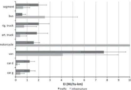
EIestimates by vehicle type are calculated using Eqs.(4) and (5)(Fig. 1) and broken down by trafﬁc and transport infra-structure use. Large differences in averageEIin terms of mega-joules consumed per tu-km can be seen between vehicles. The calculations suggest Spain’s tolled highway sections require 2.6 MJ/tu-km; 0.6 infrastructure and 2.0 trafﬁc use of energy, varying between 1.4 for diesel cars, and 29.1 for motorcycles. Similarly, in aggregate, gasoline car and diesel van transport requires between 1.6 and 11.8 MJ/tu-km; values are similar to those found inSaari et al. (2007)andPérez-Martínez and

Sor-ba (2010).

Considering traffic use, as expected, mass passenger modes consume less energy per transport unit than private transport, while for freight transport articulated trucks consume much less energy per tu-km than vans. But there are large variation in energy consumption per transport unit, depending on vehicle and fuel type; buses haveEIvalues similar to those for trucks and gasoline cars have values of over 1.6 MJ/tu-km. Considering combined traffic and infrastructure use, the most inefficient modes using gasoline and diesel technologies are motorcycles and diesel vans, due to their low load factors. Considering only infrastructure use, motorcycles, vans and buses consume more energy per transport unit due to low AAHTs. Differences inEI

between passenger and freight transport modes are similar for gasoline- and diesel-powered vehicles.

In terms of statistical significance, ANOVA test confirm significance of the meanEIand that theEIestimates for the twos slope differ and increase with slope. Similarly, the energy consumption estimates for the toll highway sections for the 10% and 30% level of HDVs show an increasing and highly significant trend. Significant differences between vehicle types, section energy consumption, andEIestimates are also observed. Sensitivity analysis of the input parameters defining energy con-sumption in Eq.(1)andEIin Eq.(3)show that increasing the input parameters by 20% results energy consumption increases significantly by 13.3%, 12.7% and 8.6%, while increasing the input parameters by 20%,EIincreases by 9.3%, 7.0%, 6.3% and 5.8%.

4. Conclusions

The paper has examined the energy consumption and interurban toll highway transport in Spain. The energy intensities of the 202 sections studied carry 79.1% of trafﬁc on the country’s toll highways but relatively little trafﬁc compared with free

(5)

highways;EIvalues for cars are many times lower than those for motorcycles. The energy intensity of buses is signiﬁcantly higher than that of cars because of the greater infrastructure resources required. Equally, while theEIvalues for articulated trucks are signiﬁcantly lower than those for rigid trucks, the values for vans are many times higher likely because of capacity variations across the vehicle types. Regarding the various road sections most of the differences found inEIare due to the highways’ slopes.

References

Boriboonsomsin, K., Barth, M., 2009. Impacts of road grade on fuel consumption and carbon dioxide emissions evidenced by use of advanced navigation

systems. Transport. Res. Rec. 2139, 21–30.

Burguess, S.C., Choi, M.J., 2003. A parametric study of the energy demands of car transportation. Transport. Res. Part D 8, 21–36.

Cenek, P.D., 1994. Rolling Resistance Characteristics of New Zealand Roads. Transit New Zealand Research Report PR3-001, Wellington.

EMEP/CORINAIR, 2009. Emission Inventory Guidebook, third ed., September 2009 Update. Technical Report. European Environment Agency, EEA, Copenhagen.

González Díaz, M.J., García Navarro, J., 2009. Criteria and methodology for an indicator of energy applied to motorways. Presented at 2nd International Conference Ravage of the Planet 2009, Cape Town.

Kühlwein, J., Friedrich, R., 2005. Trafﬁc measurements and high-performance modelling of motorway emission rates. Atmos. Environ. 39, 5722–5736.

MFO, 2009a. Trafﬁc Map, Transport and Postal Services 2008. Ministry of Development, Publications Centre, General Technical Secretariat, Madrid. MFO, 2009b. Monitoring of Road Passenger Transport and Continuing Survey of Road Freight Transport 2008. Publications Centre, General Technical

Secretariat, Ministry of Development, Madrid.

MMA, 2009. Inventory of Greenhouse Gases in Spain-Edit 2009, Summary of Results. General Environmental Quality Branch, Ministry of Environment, Madrid.

Ntziachristos, L., Samaras, Z., 2000. COPERT III Computer Programme to Calculate Emissions from Road Transport. European Environment Agency,

Copenhagen.

Park, S., Rakha, H., 2006. Energy and environmental impacts of roadway grades. Transport. Res. Rec. 1987, 148–160.

Pérez-Martínez, P.J., Sorba, I., 2010. Energy consumption of passenger land transport modes. Energy Environ. 21, 577–600.

Saari, A., Lettenmeier, M., Pusenius, K., Hakkarainen, E., 2007. Inﬂuence of vehicle type and road category on natural resource consumption in road transport.

Transport. Res. Part D 12, 23–32.