Temporal self-imaging effect for periodically modulated trains of pulses

Temporal self-imaging effect for periodically

modulated trains of pulses

S. Tainta, M. J. Erro, M. J. Garde, and M. A. Muriel

Abstract: In this paper, the mathematical description of the temporal

self-imaging effect is studied, focusing on the situation in which the train of pulses to be dispersed has been previously periodically modulated in phase and amplitude. It is demonstrated that, for each input pulse and for some specific values of the chromatic dispersion, a subtrain of optical pulses is generated whose envelope is determined by the Discrete Fourier Transform of the modulating coefficients. The mathematical results are confirmed by simulations of various examples and some limits on the realization of the theory are commented.

References and links

1. L. K. Oxenlowe, H. Ji, M. Galili, M. H. Pu, H. Hu, H. C. H. Mulvad, K. Yvind, J. M. Hvam, A. T. Clausen, and P. Jeppesen, "Silicon photonics for signal processing of Tbit/s serial data signals," IEEE J. Sel. Top. Quantum Electron. 18(2), 996-1005 (2012).

2. S. J. B. Yoo, R. P. Scott, D. J. Geisler, N. K. Fontaine, and F. M. Soares, "Terahertz information and signal processing by RF-photonics," IEEE Tran. Terahertz Sci. Technol. 2(2), 167-176 (2012).

3. P. J. Delfyett, I. Ozdur, N. Hoghooghi, M. Akbulut, J. Davila-Rodriguez, and S. Bhooplapur, "Advanced ultrafast technologies based on optical frequency combs," IEEE J. Sel. Top. Quantum Electron. 18(1), 258-274 (2012).

4. A. E. Willner, O. F. Yilmaz, J. A. Wang, X. X. Wu, A. Bogoni, L. Zhang, and S. R. Nuccio, "Optically efficient nonlinear signal processing," IEEE J. Sel. Top. Quantum Electron. 17(2), 320-332 (2011).

5. R. S. Tucker and K. Hinton, "Energy consumption and energy density in optical and electronic signal processing," IEEE Photonics J. 3(5), 821-833 (2011).

6. J. W. Goodman, Introduction to Fourier Optics (Roberts and Co., 2005).

7. A. M. Weiner, "Femtosecond optical pulse shaping and processing," Prog. Quantum Electron. 19(3), 161-237 (1995).

8. A. M. Weiner and A. M. Kan'an, "Femtosecond pulse shaping for synthesis, processing, and time-to-space conversion of ultrafast optical waveforms," IEEE J. Sel. Top. Quantum Electron. 4(2), 317-331 (1998). 9. B. H. Kolner, "Space-time duality and the theory of temporal imaging," IEEE J. Quantum Electron. 30(8),

1951-1963 (1994).

10. A. Papoulis, Systems and Transforms With Applications in Optics (McGraw-Hill, 1968).

11. S. A. Akhmanov, A. P. Sukhoruk, and A. S. Chirkin, "Nonstationary phenomena and space-time analogy in nonlinear optics," Sov. Phys. JETP-USSR28, 748 (1969).

12. E. B. Treacy, "Optical pulse compression with diffraction gratings," IEEE J. Quantum Electron. 5(9), 454^158 (1969).

13. B. H. Kolner and M. Nazarathy, "Temporal imaging with a time lens," Opt. Lett. 14(12), 630-632 (1989). 14. C. V. Bennett and B. H. Kolner, "Principles of parametric temporal imaging - Part I: System configurations,"

IEEE J. Quantum Electron. 36, 430-437 (2000).

15. C. V. Bennett and B. H. Kolner, "Principles of parametric temporal imaging - Part II: System performance," IEEE J. Quantum Electron. 36, 649-655 (2000).

16. R. Salem, M. A. Foster, A. C. Turner, D. F. Geraghty, M. Lipson, and A. L. Gaeta, "Optical time lens based on four-wave mixing on a silicon chip," Opt. Lett. 33(10), 1047-1049 (2008).

17. J. van Howe and C. Xu, "Ultrafast optical signal processing based upon space-time dualities," J. Lightwave Technol. 24(7), 2649-2662 (2006).

18. M. A. Foster, R. Salem, and A. L. Gaeta, "Ultrahigh-speed optical processing using space-time duality," Opt. Photon. News 22(5), 29-35 (2011).

20. A. V. Mamaev and M. Saffman, "Selection of unstable patterns and control of optical turbulence by Fourier plane filtering," Phys. Rev. Lett. 80(16), 3499-3502 (1998).

21. M. A. Muriel, J. Azaña, and A. Carballar, "Real-time Fourier transformer based on fiber gratings," Opt. Lett. 24(1), 1-3 (1999).

22. J. Azana and M. A. Muriel, "Real-time optical spectrum analysis based on the time-space duality in chirped fiber gratings," IEEE J. Quantum Electron. 36, 517-526 (2000).

23. R. Salem, M. A. Foster, A. C. Turner-Foster, D. F. Geraghty, M. Lipson, and A. L. Gaeta, "High-speed optical sampling using a silicon-chip temporal magnifier," Opt. Express 17(6), 4324-4329 (2009).

24. K. Goda and B. Jalali, "Dispersive Fourier transformation for fast continuous single-shot measurements," Nat. Photonics 7(2), 102-112 (2013).

25. J. Azana, N. K. Berger, B. Levit, and B. Fischer, "Spectro-temporal imaging of optical pulses with a single time lens," IEEE Photon. Technol. Lett. 16(3), 882-884 (2004).

26. R. Salem, M. A. Foster, and A. L. Gaeta, "Application of space-time duality to ultrahigh-speed optical signal processing," Adv. Opt. Photon. 5(3), 274-317 (2013).

27. S. Thomas, A. Malacarne, F. Fresi, L. Poti, and J. Azana, "Fiber-based programmable picosecond optical pulse shaper," J. Lightwave Technol. 28(12), 1832-1843 (2010).

28. J. Azaña, "Design specifications of time-domain spectral shaping optical system based on dispersion and temporal modulation," Electron. Lett. 39(21), 1530-1532 (2003).

29. C. Wang and J. P. Yao, "Chirped microwave pulse generation based on optical spectral shaping and wavelength-to-time mapping using a Sagnac loop mirror incorporating a chirped fiber Bragg grating," J. Lightwave Technol. 27(16), 3336-3341 (2009).

30. H. Chi and J. Yao, "All-fiber chirped microwave pulses generation based on spectral shaping and wavelength-to-time conversion," IEEE Trans. Microwave Theory 55(9), 1958-1963 (2007).

31. Y. Park, T. J. Ahn, J. C. Kieffer, and J. Azaña, "Optical frequency domain reflectometry based on real-time Fourier transformation," Opt. Express 15(8), 4597-4616 (2007).

32. H. F. Talbot, "Facts relating to optical science no. IV," Philos. Mag. 9, 401-407 (1836).

33. L. Rayleigh, "On copying diffraction gratings and on some phenomenon connected therewith," Philos. Mag. 11(67), 196-205 (1881).

34. M. V. Berry and S. Klein, "Integer, fractional and fractal Talbot effects," J. Mod. Opt. 43(10), 2139-2164 (1996).

35. M. S. Chapman, C. R. Ekstrom, T. D. Hammond, J. Schmiedmayer, B. E. Tannian, S. Wehinger, and D. E. Pritchard, "Near-field imaging of atom diffraction gratings: the atomic Talbot effect," Phys. Rev. A 51(1), R14-R17(1995).

36. J. Wen, Y. Zhang, and M. Xiao, "The Talbot effect: recent advances in classical optics, nonlinear optics, and quantum optics," Adv. Opt. Photon. 5(1), 83-130 (2013).

37. T. Jannson and J. Jannson, "Temporal self-imaging effect in single-mode fibers," J. Opt. Soc. Am. 71, 1373-1376(1981).

38. J. Azaña and M. A. Muriel, "Temporal Talbot effect in fiber gratings and its applications," Appl. Opt. 38(32), 6700-6704 (1999).

39. J. Azaña and M. A. Muriel, "Temporal self-imaging effects: Theory and application for multiplying pulse repetition rates," IEEE J. Sel. Top. Quantum Electron. 7(4), 728-744 (2001).

40. J. Azaña and L. R. Chen, "General temporal self-imaging phenomena," J. Opt. Soc. Am. B 20(7), 1447-1458 (2003).

41. D. Pudo and L. R. Chen, "Tunable passive all-optical pulse repetition rate multiplier using fiber Bragg gratings," J. Lightwave Technol. 23(4), 1729-1733 (2005).

42. J. Caraquitena and J. Marti, "High-rate pulse-train generation by phase-only filtering of an electrooptic frequency comb: Analysis and optimization," Opt. Commun. 282(18), 3686-3692 (2009).

43. J. Caraquitena, Z. Jiang, D. E. Leaird, and A. M. Weiner, "Tunable pulse repetition-rate multiplication using phase-only line-by-line pulse shaping," Opt. Lett. 32(6), 716-718 (2007).

1. Introduction

Photonic Signal Processing [1-5] is becoming today one of the most active research topics in optics and photonics, as all-optical processing offers a better performance for high-speed signals than electronic alternatives. Many well-established techniques for optical processing are based on volume optics, employing schemes that combine the diffraction of optical beams propagating through free space, thin lenses and prisms. This area of optics is highly developed and is usually known as Fourier Optics [6-8]. However, volume optics presents several drawbacks associated to the use of bulk optical components, which have to be carefully aligned and occupy a large space.

the formal equivalence of the mathematics that govern the paraxial diffraction of beams propagating through free space and the dispersion in time of narrowband pulses through dielectric media. Although this duality was already described in the late 1960s, it has been mainly in the last two decades when it has started showing its full potential, especially after the extension of the duality to include the "time lens", that is, the equivalent in the temporal domain to a conventional spatial thin lens [13-16]. Since then, scientists have developed numerous photonic processing systems, using integrated and robust optical waveguide components [17-20]. Among these proposals, the Optical Fourier Transform and the temporal self-imaging effect have gained a special attention as candidates for the processing of single optical pulses and optical trains of pulses.

In many signal processing applications based on Fourier optics, the ability to generate the Fourier transform and its inverse for a given signal are essential for the operation of the system. In space optics, a simple approach to obtain the Fourier transform of an object is the use of Fraunhofer diffraction. The basic idea is that far-field diffraction of an object produces the formation of its Fourier transform in the transverse space [6]. This scheme can be replicated in the time domain by simply passing a time-limited waveform through a highly dispersive medium, mapping the spectral information of the signal to the time domain. The proposal of this real-time Fourier transformer, also known as frequency-to-time converter, was made by Muriel et al. [21, 22] who were the first to use a chirped Fiber Bragg Grating as the dispersive device. The realization of the Fourier transform by means of a dispersive medium in the optical domain has found several applications, such as the realization of temporal magnification systems, causing the waveform to be stretched in time and allowing thus the single-shot characterization of ultrafast waveforms [23-26]. In combination with electro-optic modulation, this setup can also perform the temporal and spectral shaping of optical pulses [27-31].

Temporal self-imaging is another popular development of temporal optical processing systems. The Talbot effect or self-imaging effect is a near-field diffraction effect that was first reported by H. F. Talbot in 1836 [32]. When a coherent plane wave is passed through or reflected by a ID or 2D periodic object, an exact image of the object can be observed at regular distances [33-36]. Also, sub-images of the object can be observed at shorter distances where, depending on the distance, a certain reduction of the image size is presented. As the spatial Talbot effect is a diffractive effect, an equivalent outcome occurs when a periodic signal, such as a train of optical pulses, is passed through or reflected by a dispersive medium. This result is known as temporal Talbot -or temporal self-imaging effect. Being first proposed and demonstrated by Jannson et al. [37] and generalized in [38-40], it has been broadly studied and has gained a special interest for the multiplication of the repetition rate of an optical train [41-43].

section 4 numerical simulations that show the validity of the proposal are presented and some of its possible applications for the processing of optical trains of pulses are outlined. Finally, a summary of the most important results is provided in Section 5.

2. Temporal self-imaging effect for modulated pulses

In this section, the temporal self-imaging effect when the train of optical pulses at the input of the system has been previously modulated will be studied. As hypothesis, it will be assumed that a train of optical pulses with equal phase and amplitude has been modulated by a complex signal, c(t). Thus, the complex envelope of this signal, x(t), is given by:

x{t) = c{t)Yja{t-kT0) (1)

where a(t) is the individual shape of each pulse, T0 is the repetition period and c(t) is the

complex modulating signal and, in consequence, applies a different phase and amplitude to every pulse. The pulse width of each individual pulse, At, which is determined by a(t), is considered to be small enough so that the pulses will not overlap, that is, At<T0. Also, two

additional restrictions are imposed to c(t):

• c(t) has to be periodic and its period is given by NT0, where TV is an integer

c(t) = c(t + NT0) (2)

• c(t) is a slow signal when compared to the duration of the individual pulses, At, so that it it can be considered as constant within the duration of an individual pulse:

c(t) ~ c(kT0 ) = ck for kT0 <t< kT0 -\ where k is an integer (3)

By introducing conditions (2) and (3) to Eq. (1), the signal at the input of the system can be expressed as the summation of TV different trains of pulses with periodicity Tx = NT0, a

temporal delay between each train of T0 and being each of them modulated by a different

coefficient c,. Accordingly, it is possible to group the pulses in TV different trains, each with constant phase and amplitude:

*C)=E

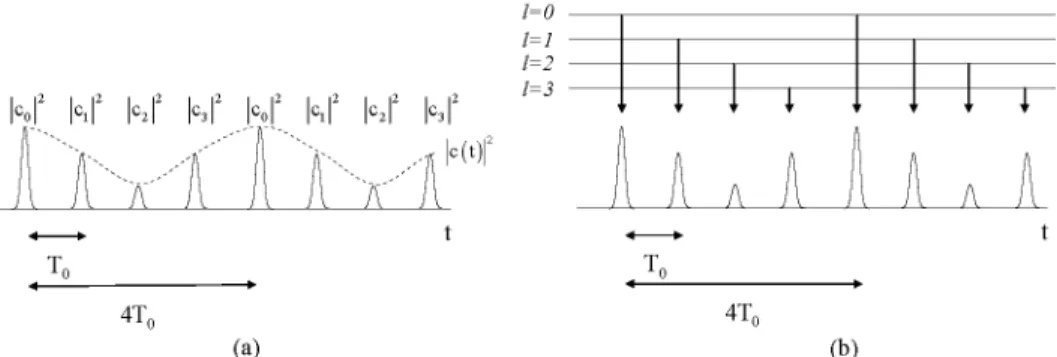
An example of such grouping can be observed in Fig. 1, when the input train of pulses is modulated by a signal c(t) with periodicity 4T0. As a result of this, it is possible to regroup

the pulses in four different trains each one modulated by a fixed coefficient c, (I = 0,1,2,3),

which is determined by the value of c(t) in / = IT0 . As a consequence of this rearrangement

1=0 1=1 1=2 1=3

X

i

JL

•4 •

T

1 n

4T„ 4T„

(a) (b)

Fig. 1. (a) Train of pulses that have been intensity modulated by a set of coefficients with N =

4 and (b) grouping of the different trains depending on the modulating coefficient.

2.1 Temporal self-imaging

As all the trains of pulses defined by / in Eq. (4) have a similar period, Tx, the amount of

dispersion required in order to obtain the temporal self-imaging effect [38] for every one of them is given by:

E1-.

In In = ± 1 + 2 + 3 . (5)

where, depending on the value of s, two different cases can be distinguished: the ordinary and the inverted temporal self-imaging effect.

When s is even, the obtained result is the ordinary temporal self-imaging effect for each of the subtrains defined in Eq. (4) inside the brackets. As a consequence, each train produces after the dispersion a train of pulses modulated by the corresponding coefficient c, and with

no additional temporal delay. Therefore, the signal at the output of the system, y(t), can be expressed as:

y{t) = Y c^ait-w.-n,

Due to the time delay IT0 between the different trains, the pulses coming from the

different trains will not overlap in time, not existing any interference between the trains of pulses. Thus, the output of the system is a replica of the train at the input, maintaining the same modulating coefficients than the input train, and the detected optical power at the output of the system is given by:

^,W=£hf ZK'-^i-'-To

Similarly, when s is odd, each of the N trains in which the total signal has been decomposed is affected by the inverted temporal self-imaging effect. As a result, each of the trains produces at the output another train of pulses also modulated by the corresponding coefficient c, but with an extra delay of Z¡ ¡2 . The signal at the output of the system can be expressed as:

As in the case of the ordinary self-imaging effect, the train of pulses at the output of the system is a replica of the train at the input, but in this case with an additional time delay of

Tx¡2 . Therefore, the optical power at the output of the system is:

i V - l |2

¿U')=Xl

/l XK'-*?;-^0-71/2)1 (9)

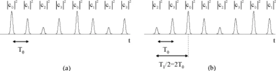
In Fig. 2 an example for both (a) s even and (b) odd can be observed. In the first case the train of pulses obtained at the output is a replica of the input train, whereas in the second an additional Tj2 delay appears. These results can also be understood by considering

i V - l

a'(/) = ^ [ c;- a ( / - / 7, 0) ] as the shape of a single pulse of the total train. Under this

1=0

condition, the input train of pulses can be interpreted as an unmodulated train of pulses whose pulse shape is determined by a'(t) and with a periodicity Tx. Therefore, by applying

the dispersion given by Eq. (5), the train of pulses will suffer the integer self-imaging effect, which corresponds to the obtained results. That is, these results can be simply considered as the particular case of the integer temporal self-imaging effect for which there are non-equal amplitude or phase pulses. It is worth noting that the condition for the dispersion is given by Eq. (5), that is, the usual value for the integer temporal self imaging effect is used but with the period of the modulating signal, Tx, and not the temporal separation between consecutive

pulses, T0.

A A l\ l\ A A A l\ l\ A A

(a) T l / 2 2T° (b)

Fig. 2. Output of the system, for the input train shown in Fig. 1, when (a) s is even or (b) s is odd.

2.2 Fractional temporal self-imaging

Depending on the amount of dispersion applied to the input train of pulses, it is also possible to obtain the fractional temporal self-imaging effect for each of the N train of pulses in Eq. (4). In this case, the required condition for the dispersion [38] is given by

7f s=NX s ¡s = ±l,±2,±3... ( i o )

2K m 2K m [ m =2,3,4...

where s/m is an irreducible fraction. Also, in order to avoid the overlapping of adjacent pulses after the dispersion, an additional restriction has to be imposed to the duration of the pulses, limiting it to a fraction of the output repetition rate determined by m :

T T

At<^ = ^ - (11) m mN

As in the study of the temporal self-imaging effect for unmodulated trains, two different scenarios depending on the value of the product s • m have to be studied: the ordinary and the inverted fractional temporal self-imaging effects.

whose intensity repetition rate is given by Tjm = NT0/m and without any additional

temporal delay is obtained for each subtrain. Hence, the resulting train of pulses for each value of / can be expressed as [38]:

c^Aatt-k^-lT,) (12)

where Ak are the coefficients associated to the temporal self-imaging effect and are given

by:

4=!gexpi/-J^-34] (13)

mq=0 \ [m m })

As a result of this, the signal at the output of the system is determined by the superposition of these trains:

y{t)=Y

H

At-k-T

-lT

\ (14)

kTL££ y m )

It is worth emphasizing that, although the intensity repetition rate has been multiplied by a factor m, the term in Eq. (13) introduces a different phase shift for each subtrain, resulting thus in a train whose periodicity is Tx, as in the original train.

On the other hand, if s • m is odd, each train of pulses is affected by an inverted fractional temporal self-imaging effect. Consequently, each of the N trains of pulses results at the output in another train whose intensity repetition rate is given by Tx ¡m = NT0 ¡m and with an

additional delay of Tx /2m :

c^sJi-k^-lT,-^-) (15)

¿~L v m 2m)

where the coefficients Bk are given by:

is 7 2k+1

Bk=— 2_QMJ7V\— q + q

mq=0 \ [m m

Finally, the signal at the output of the system is determined by

(16)

- «-i ( N N \

y{t) = X i > M

~

-

° ~

° ~^

°

*«o/=o V m 2m J

As it can be observed in Eqs. (14) and (17), the outcome in both cases is the superposition of N trains of pulses whose intensity repetition rate is given by Tx ¡m = NT0 ¡m and a delay

between each subtrain of T0. Consequently, the profile of the trains is going to be determined

by the relation between m and N. Also, if N/m is an irreducible fraction, there would be no interaction between the different subtrains, so that the amplitudes of the pulses at the output can be directly determined by the coefficients c,Ak or c,Bk. However, if N/m is a

reducible fraction, then the pulses coming from different subtrains will occupy the same time slot, overlapping in time and producing interference between the different subtrains due to the different phase terms associated to each of them. In consequence, the optical power of the pulses at the output cannot be evaluated to obtain a general expression, since the coefficient modulating each pulse is now given by the sum of several coefficients c,Ak or c,Bk.

optical power, as we will be doing in the next section for a specific case that is of special interest.

3. Discrete Fourier transform of the modulating coefficients

In the previous section, it has been demonstrated that, when the fractional temporal self-imaging condition determined by Eq. (10) is verified, the train of pulses at the output presents an intensity repetition rate given by Tx ¡m = NT0 ¡m, which depends on the relation

between m and N . In this section, the case for 5 = 1 and m = N2 is going to be studied.

This case is specially interesting because the amount of dispersion which is applied has a fixed value <j> = T2 ¡In , being thus independent on the number of coefficients modulated to

the input train, N, and on the period of the modulating signal, Tx. As in the previous section,

depending on the value of sm being even or odd, two different cases have to be studied. In the first case, N is going to be considered even. In consequence, the product

s-m = N2 is also going to be even, and the train of pulses at the output will be given by Eq.

(14). Therefore, by inserting the aforementioned conditions for s and m into this expression and introducing k' = k+lN, the train of pulses at the output can be expressed as a single train of pulses whose repetition rate is given by T0/N :

*(0=I ÍX/

/

EH'-*§)

(18)

and the coefficients nk, can be expressed as:

iV-liV2-l

^ - t Z ^ e x p í y ^ + íl*'-^),}

1=0 q=0

N

1 N -1

q=0

Sc,exp|-;y/? exp lj-^{q2+2k'q]

(19)

Additionally, by introducing the variables w and z , defined to be two integer numbers that verify q = w + zN, the first sum term can be divided in two summations, obtaining:

"'•=T»T T\T,c¡exp(j^{(w + zN)2+(2k'-2lN)(w + zN)}

JV w=a z=a ;=n V N w=0 z=0 L '=0

iV-1

A^

l Z H ; 7 >

+ 2 * M Í :

Í l7ti

(20)

I

Thus, by rearranging the different terms in Eq. (20), the coefficients nk, can be rewritten

as:

^=-^ikexpi^K

2^jl|:

-l)zexp| j-?-z{w + k'} (21)

where Cw can be identified as the w-th term of the Discrete Fourier Transform of the

C „ , = Í >;e x p -1—lw In,

N

(22)

To further work with this expression, it is demonstrated in the Appendix that the summation inside the inner brackets can only have two possible values depending on the value of the complex exponential:

X ( - l )Ze x p ^ z {W + r }

0 if w±rN-k'+

N if w = rN-k'+ N_

2 N_

2

(23)

where r is an integer. In order to determine which terms of the summation within nk, are

non-zero, the values where the condition w = rN - k'+ N/2 is verified have to be found. Due to the external summation in Eq. (21), w is restricted to be an integer between 0 and N -1, i. e., 0 < w < N-l. Therefore, given a certain value of k', the possible valid values for r are going to be limited to the interval:

k'-N/2

k'+N/2-• </ •<• 1 (24)

N N

As it can be seen, the size of the interval in Eq. (24) is (N-l)/N, which is going to be inferior to the unity. Therefore, as r has to be an integer, there is only one possible value of r within the interval, r0, which verifies the condition w = rN-k'+ N/2. As this value is

unique, it also determines the single possible value of w , w0, that, for a fixed value of k',

verifies the necessary conditions for the inner summation in Eq. (21) to be different than zero:

Wn -•r0N + N •k' (25)

In consequence, the external sum of Eq. (21) is reduced to a single summand whose index is determined by w0 and that has a value of N according to Eq. (23). Therefore, the

coefficient^, can be simplified to:

"f=^CWoexp{j^{w20+2w0k'}

1

CA, .71

And the signal at the output of the system, given in Eq. (18), thus results into: ^ ^ e x p ^ i e x p _-J%

(26)

y(')= ¿ 7 7_, C^e x P | ^ le xP

Í V 2

• (k'

-J7Z\ —

{N <\2"\

a\t-k^ N

(27)

Introducing the variable k" = N/2 - k' and considering that the pulse width is small enough so that pulses don't overlap (At < T0 ¡N), the optical power at the output of the

system can be finally expressed as:

PoAt)

N2

TK

alt + k"^-7 ^-N 2

The second case to be considered is when N is odd, which corresponds to the inverted fractional temporal self-imaging effect. Under this assumption, the product s-m = N2 is

going to be odd, so the output train of pulses is determined by Eq. (17). As in the previous case, the output can be expressed as a single train of pulses whose repetition rate is given by

TJN:

y(t)=Y

ÍX/v

a\t-k'^--^-N 2a\t-k'^--^-N ( T T

* £ t { N 2N

with k' = k + lN and where the coefficients mk, are given by:

N-l N2 -1

(29)

N'f v ;=n a=a V Jv 0 q=0

N

1 i V2- l

q=0

.In,

exdj^{q2+{2k'+l)q}

(30)

Y e , e x p

-j-In order to further simplify this expression and following a similar procedure as in the even case, the variable w = q - zN with z an integer is introduced in the equation, so that by rearranging the terms of the summations the following equation is obtained:

m,r

^1M^{,,.

+

,,(«,1)}

Af

(31)

where Cw corresponds again to the w-th term of the Discrete Fourier Transform of the

coefficients c,. The inner summation can be fiirther simplified using the relation demonstrated in the Appendix, which results in:

X ( - l )ze x p ( ^ z ( 2W + 2£'+l

Af

0 if w*rN-k'+

N if w = rN-k'+ N-l

2

N-l (32)

and the interval for the possible values for r so that the summation is non-zero is now:

£ ' - ( A f - l ) / 2 k'+(N-1)2

<r<-N N

(33)

As in the previous case, there is only one integer value r0 with its corresponding w0 that

verifies this condition, and Eq. (31) can be simplified to:

m,r

^

e x p O - ^ K

( 2 * ' + l ) }

A^

J.

A^ C, ' ! >

(34)

p„„, (t)

I

I

system can be expressed as:

_J_

(N-l)/2 C,

T N

a\ t IN J

T -k'-±-N

T

J_o_

2N

(35)

- k', the resulting optical power at the output of the

P„„, It) 1

Z I Q

of the train at the output of the system is similar regardless of the parity of N. In both cases, the separation between consecutive pulses is going to be determined by T0 fN, that is, by the

number of coefficients modulated to the train at the input, and an additional T0/2 delay is

introduced to the output train. Also, the amplitude of the pulses at the output of the system is going to be determined by the Discrete Fourier Transform (DFT) of the modulating coefficients c, applied in reverse order. It is worth recalling that in this case, the required dispersion depends only on the repetition rate at the input of the system, regardless of the number N of modulating coefficients. Thus, by modifying only the coefficients c, that are determined by an easily tunable electrical signal, it is possible to simultaneously control the amplitude and repetition rate at the output, as it can be seen in Fig. 3.

\cj icr ic„r \c

3T„

T„/3

(a) (b)

Fig. 3. (a) Train of pulses modulated at the input of the system with N = 3, and (b) at the output of the system.

4. Numerical simulations

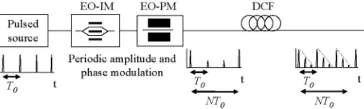
To verify the validity of the proposal, the system shown in Fig. 4 was evaluated using Matlab. The simulated pulsed source produced a train of Gaussian optical pulses operating at a repetition rate T0=l00ps ( /0= 1 0 G H z ) and a pulsewidth of 1 ps. The train was

modulated using two ideal electro-optic modulators to modify both the amplitude (intensity modulator) and phase (phase modulator) of each pulse, assuming neither bandwidth restrictions nor modulator losses. As the modulation was done both in phase and amplitude, the coefficients were evaluated using the DFT of the desired envelope to be obtained at the output, as demonstrated in the previous section. Finally, the modulated signal was dispersed using 15.6 km of Dispersion Compensating Fibre (DCF) with « = 0.55dB/km,

D = -80 ps/nm/km, 5' = 0.19ps/nm2/km, which corresponds approximately to the total

Pulsed source

EO-IM

^

EO-PM

^m

^

DCF

am)

Periodic amplitude and

phase modulation J L

NT„

[MML

NTn

Fig. 4. Proposed setup with intensity and phase modulation in the time domain followed by a dispersive device (EO-IM: Electrooptic Intensity Modulator, EO-PM: Electrooptic Phase Modulator, DCF: Dispersion Compensating Fibre).

In Fig. 5 the pulses (a) at the input and (b) at the output of the system when no modulating signal is applied are presented. As it can be observed, the signal at the output of the system corresponds to a train of pulses with the same repetition rate as the input and an additional T0/2 delay. This result was expected, as this scenario corresponds to the

self-imaging effect when the parameters 5 = 1 and m = \, which corresponds to the inverted case analyzed in section 2.1. Also, as a result of the DCF third order dispersion, the pulses present the typical deformation associated to it, showing some ripples at one side of the pulses.

10 o 1.0

1 °-

» „ ,

a

100 Time (ps)

(a)

200 100 Time (ps)

(b)

200

Fig. 5. Train of pulses at the input (a) and at the output (b) of the system when no modulation is applied.

Initial simulations were done using only intensity modulation and binary c, coefficients. In Fig. 6 the train of pulses obtained at the output of the system for the coefficients (a) 1000000000 and (b) 1000000001 can be seen, as well as the expected output envelope (dashed line) obtained by the DFT of the different modulating coefficients that have been applied. As expected, the train of pulses at the output presents a time delay of T0 ¡2, that is,

50 ps and the repetition frequency is multiplied by a factor N = 10, resulting in a separation between pulses of only 10 ps. However, as the pulse width at the input was 1 ps, no overlapping occurs despite the smaller separation between the pulses. Also, the envelope of the output train of pulses has been modulated, obtaining a constant signal and a cosine signal envelope, respectively, which correspond to the DFT of each of the modulated coefficients.

0.01

o.oo

200

0.04

0.02

0.00 200

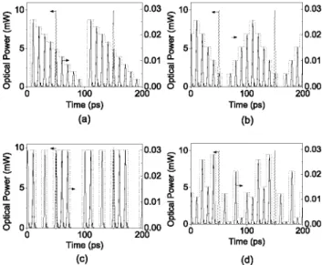
In order to further verify the shaping capabilities of the setup, four different functions were chosen to be obtained as envelopes at the output of the system: a ramp envelope, a triangular envelope a burst of binary data (1001110101) and a signal with random amplitudes, in all cases with TV = 10. The modulating coefficients were evaluated using the DFT of the desired output envelope in each case. The obtained trains at the output of the system can be seen in Fig. 7, obtaining that the peak power of the output pulses corresponds to the DFT of the modulating coefficients that were chosen for the example but in reverse order, as expected.

o.oo 200

10

! 5 o o

100 Time (ps)

(c)

0.03 10 E 0.02

0.01

1 5

Q_

0.00 o o

200 100 Time (ps)

(d)

0.03

0.02

0.01

0.00 200

Fig. 7. Train of pulses at the input (dashed) and output (solid) of the system and the expected output envelope (dotted) for a (a) ramp, (b) triangular, (c) binary data and (d) random envelope.

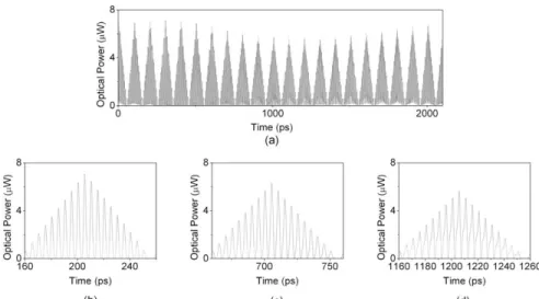
In the previously presented examples the pulse width and the repetition factor were small enough so that there was no overlapping between adjacent pulses. However, if the number of modulating coefficients TV is increased, the condition given by Eq. (11) will not be fulfilled, appearing interference between adjacent pulses and invalidating the result obtained in Eq. (36). Two examples where this interference is significant can be seen in Fig. 8 and Fig. 9, where TV = 20 and TV = 60 respectively, and the modulating coefficients were chosen to obtain a triangular envelope at the output. As it can be seen, in the first case the pulses do not overlap completely, but a small amount of interference appears due to the sidelobes resulting from third order dispersion. The effect of this interference is a degradation of the peak optical power obtained in some of the pulses.

On the other hand, when the number of coefficients is high enough (TV = 60 in Fig. 9), the pulses completely overlap, resulting in a complete interference between them. When the phases between adjacent pulses don't differ too much, the pulses overlap in power, obtaining a single pulse with the shape of the envelope instead of a train of pulses (see Fig. 9(b)). Yet, when the phases of the adjacent pulses diverge, the different pulses interfere with different phases and the signal at the output presents a noisy behavior, showing very fast power fluctuations and a general loss in the obtained peak optical power (Fig. 9(c)). This behavior is periodic, as the phases of the coefficients nk, and mk, from Eqs. (26) and (34) present a

periodicity TV2, resulting in a periodicity for the output train determined by NT0 (6000 ps in

%4

O O

200 240 Time (ps)

(b)

I

Q.

o o

Lá

iiik,

Time (ps)

(c)

5 4

o 0

1160 1180 1200 1220 1240 1260 Time (ps)

(d)

Fig. 8. Train of pulses at the output of the system for a desired triangular envelope with N = 20; 20 periods of the output are shown in (a) and zooms of the signal in (a) for three specific periods are shown in (b) to (d).

100 Time (ps)

(b)

150 o 0.0 3100

Time (ps)

(d)

1600 1650 Time (ps)

(C)

Fig. 9. Train of pulses at the output of the system for a desired triangular envelope with N = 60; 60 periods of the output are shown in (a) and zooms of the signal in (a) for three specific periods are shown in (b) to (d).

5. Conclusions

This work has been developed within the well-known space-time framework for the manipulation of optical pulsed trains. It has focused on a situation of special interest that cannot be considered neither a single-pulse Fourier Transform nor the repetition rate multiplication obtained by means of the temporal self imaging effect: the propagation through a dispersive element of a train of periodically modulated ultrashort pulses when different pulses interfere at the output. It has been found that, for some precise values of chromatic dispersion, the resulting outcome is composed of a periodic pulse train whose intensity repetition rate has been multiplied and whose envelope can be evaluated as the Discrete Fourier Transform of the modulating coefficients. A mathematical demonstration of this transform has been developed, showing the conditions in which it is valid.

presented, extending afterwards these results to more complex envelopes obtained employing both phase and intensity modulation and the DFT of the desired output envelope in each case. This enables the application of the proposed scheme as an optical train pulse shaper, allowing for example the generation of high-speed binary optical bursts that are of great interest in optical communication systems. Additionally, as the dispersive medium is fixed, the proposed setup could be used to modify the intensity repetition rate of the train at the output by varying only the modulating electrical signal. Furthermore, another possible area of application is the generation of arbitrary millimeter and microwave waveforms employing an envelope detector at the output of the system.

Finally, a study of the limitations of the analysis was made. More specifically, it has been demonstrated that, for a given pulsewidth, there is a maximum number of modulating coefficients that can be used, and a corresponding maximum repetition rate at the output, since otherwise adjacent pulses overlap and the interference prevents the formation of the desired Discrete Fourier Transform. However, it has been found that under these conditions, the system operates as an optical pulse shaper, allowing the synthesis of at least one optical pulse in each period of N with the desired envelope, a finding that will need further research.

Appendix

Previously, in order to simplify the resulting mathematical expression for the superposition of different trains of pulses when 5 = 1 and m = N2, the mathematical identities of Eqs. (23)

and (32) were imposed for N even and odd, respectively. For the completeness of the demonstration, in this appendix the full derivation of these expressions will be presented. Introducing s' = 2w + 2k' for Eq. (23) and s' = 2w + 2k'+l for Eq. (32), it is possible to unify both expressions as:

"-' .h ( _n \ Í0 s'*(2r + l)N

Y ( - l ) " e x p | j—hs'\ ,

^y ' ! N ) \N s' = (2r + V)N

(37)

Also, it will be proven that this equality is only valid as long as s and N have the same parity. As it can be observed, due to the definition of s' for N even and odd, this condition is fulfilled by Eqs. (23) and (32). To continue the analysis, two different cases are going to be considered depending on N being even or odd.

If N is assumed to be even, then the summation can be divided in two different summations by selecting the summands depending on h being odd or even:

Z(

tí

V N

n

-expl / — s

1 N

(38)

As it can be observed, a summation of complex exponentials is obtained. In order to calculate its value, we only need to use the well-known mathematical identity that exists for the summation of geometric series:

M-\

z=0

\-cf_

I —a (39)

where, in our case, a = exp(j2ns'/N). Therefore, the result of the summation in Eq. (38) is given by:

^ f .In > exp / — zs

l + e x p l y — s'

and introducing Eq. (40) in Eq. (37), it is obtained that:

, • n <

-exp /—5

1 J N

X(-l)* e x p l o t e ' l-exp(y^-5')

i ( • n i

1+exp / — s

{ N

(41)

Equally, a similar analysis can be performed when TV is odd. However, in the separation of the even and odd terms done in Eq. (38) an additional term has to been taken in consideration before grouping:

~W-1

~ ^ - ~ I .71

X ( - l ) * exp[./-^fe _{X e xp [ i T 72 z s' 1-exp /—s}

1 TV

f

-exp

,-J

~

)

\

jx

TV

(42)

As in the previous case, the summation of a complex exponential function is obtained so that it can be simplified by applying Eq. (39), which results in:

J V - 1 _ 2

X QXV\J^;2zs'

TV

1-exp jn TV-1 TV

7t

1 +e x p i y ^ 5 '

and introducing this identity into Eq. (42), the summation can be expressed as: l - e x p | j — s'

X ( - l ) * e x p i a t e ' l + exp{ jas')

1 + expiy^5'

(43)

(44)

With this result and combining it with Eq. (41), a single expression for both TV even and TV odd can be obtained:

X i - i r e x p l ^ *5'

. n

1-,(N+s')

71

1 + expl ; — s'

(45)

As it can be observed, the numerator of Eq. (45) is always going to be zero if the value of TV + s' is even, which is satisfied only when the parity of s' and TV is the same. Therefore, if both s' and TV are even or odd simultaneously, the result of Eq. (45) is going to be zero unless the denominator is also zero. In this last case, an indeterminate form is obtained and the value of the function has to be determined by using its limits at those points. This will occur only when exp(jns'/N) = - 1 , that is, when the value of the complex exponent is an odd multiple of n, which is satisfied when s '/TV corresponds to an odd number. Therefore, the limits when s' = (2r + 1)TV are going to be studied, where r is an integer number. By applying L'Hopital's rule, it is obtained that the value of the function at those points is:

lim

->(2r+l)JV

l-(-l) H m -M-l)

1 + exp| j — s'

71 i'-K2r+l)JV J! . 71 ,

j—exp j—5

TV { N

:N (46)

Therefore, if the parity of s' and TV is the same, the value of the summation is going to be:

¿ ( - t f e x p ; ^ 0 s'*(2r+l)TV

TV s' = (2r+l)TV (47)

as we wanted to demonstrate.

Acknowledgments