Order 10"^ speedup in global linear instability analysis using matrix formation
Pedro Paredes *, Miguel Hermanns, Soledad Le Clainche, Vassilis Theofilis
School of Aeronautics, Universidad Politecnica de Madrid, Pza. Cardenal Cisneros 3, E-28040 Madrid, Spain
A B S T R A C T
A unified solution framework is presented for one-, two- or three-dimensional complex non-symmetric eigenvalue problems, respectively governing linear modal instability of incompressible fluid flows in rectangular domains having two, one or no homogeneous spatial directions. The solution algorithm is based on subspace iteration in which the spatial discretization matrix is formed, stored and inverted seri-ally. Results delivered by spectral collocation based on the Chebyshev-Gauss-Lobatto (CGL) points and a suite of high-order finite-difference methods comprising the previously employed for this type of work Dispersion-Relation-Preserving (DRP) and Pade finite-difference schemes, as well as the Summation-by-parts (SBP) and the new high-order finite-difference scheme of order q (FD-q) have been compared from the point of view of accuracy and efficiency in standard validation cases of temporal local and BiGlobal linear instability. The FD-q method has been found to significantly outperform all other finite difference schemes in solving classic linear local, BiGlobal, and TriGlobal eigenvalue problems, as regards both memory and CPU time requirements. Results shown in the present study disprove the paradigm that spectral methods are superior to finite difference methods in terms of computational cost, at equal accu-racy, FD-q spatial discretization delivering a speedup of 0(10''). Consequently, accurate solutions of the three-dimensional (TriGlobal) eigenvalue problems may be solved on typical desktop computers with modest computational effort.
1. Introduction
The present contribution focuses on the application of high-or-der finite-difference methods to the numerical solution of partial-derivative eigenvalue problems (EVP) which govern global linear flow instability. The term global instability is used here to collec-tively describe instability in domains in which the number of homogeneous spatial directions is one or zero, respectively corre-sponding to two- and three-dimensional EVP. Global linear insta-bility analysis is motivated by the need to unravel the origins of laminar-turbulent transition in flows over or through complex geometries; the theory has advanced into a field of vigorous re-search activity in the last decade [1]. This endeavor has been facil-itated by the wider availability of computational resources commensurate with the solution of the multi-dimensional eigen-value and singular eigen-value decomposition problems underlying the theory. While non-modal studies of instability of complex flows have commenced appearing in the literature in recent years [e.g. 2,3], the overwhelming majority of work is performed in a modal context, governed by the solution of large-scale eigenvalue prob-lems. Their solution entails two aspects, spatial discretization and eigenspectrum computation, which are briefly reviewed next.
Corresponding author.
E-mail address: [email protected] (P. Paredes).
Regarding spatial discretizations for global instability analysis, the early flow applications analyzed involved simple two-dimen-sional domains in which the numerical discretization techniques employed were straightforward extensions of those used in the solution of classic one-dimensional linear stability eigenvalue problems. The pioneering studies of inviscid instability of a vortex by Pierrehumbert [4], viscous instability analyses in the wake of the circular cylinder by Zebib [5] and the rectangular duct by Tats-umi and Yoshimura [6] fall in this category; all three works em-ployed spectral methods for the spatial discretization of the linearized operator. Almost simultaneously, finite-element meth-ods were also used for the solution of the two-dimensional EVP by Jackson [7] and Morzyiiski and Thiele [8], while finite-volume methods soon followed [9]. Although finite-element or finite-vol-ume methods are not restricted to the single-domain two-dimen-sional grids employed in the early spectral analyses, their low formal order of accuracy needs to be compensated in terms of grid density: should sharp gradients need to be resolved, as the case is with the amplitude functions of global eigenmodes at increasingly high Reynolds numbers, one resorts to using unstructured meshes of ever-increasing density in order to achieve convergence [e.g. 10]. In doing so, one effectively trades off the efficiency of a high-order method in favor of the flexibility offered by the unstructured mesh discretization. The case is thus set for high-order accurate, flexible
Such an approach has been introduced in the seminal work of three-dimensional instability in the wake of a circular cylinder by Barkley and Henderson [11,12] in the form of spectral-element discretization on structured meshes. The first application of a spec-tral/hp-element method [13] to the study of a global instability problem on unstructured meshes was that of Theofilis et al. [14], who recovered instability in the wake of a NACA0012 airfoil as the leading BiGlobal eigenmode of the steady wake flow.
Regarding eigenspectrum computations, early analyses relied on full eigenspectrum computation [15,5], which scales as ©(M^) and 0{M^) with regard to memory and CPU time requirements, respectively, if a total number of M degrees of freedom are used for the spatial discretization of the linearized operator. Both esti-mates present a severe limitation for full eigenspectrum computa-tions in both two and three simultaneously discretized spatial directions. Access to the entire eigenspectrum of global eigenvalue problems is thus routinely sacrificed in present-day global instabil-ity analysis algorithms, which employ some form of subspace iter-ation to recover a small subset of the eigenspectrum. This practice is justified since, from a physical point of view only a relatively small part of the leading perturbations, those close to the origin, is relevant to flow instability. On the other hand access to the smallest eigenvalues implies inversion of the discretized linear operator; a common practice to avoid inversion, the cost of which is also 0{M'^) and 0{M^) if a direct dense method is used, is to emu-late the action of the inverse operator during the subspace crea-tion, without ever forming or inverting the operator. Well-established practices in the latter context, collectively referred to as time-stepping methods, have been introduced by Eriksson and Rizzi [16] and Edwards et al. [17] and are in use in modern global instability analyses, such as the three-dimensional global instabil-ity analyses ofTezukaand Suzuki [18] and Bagheriet al. [19], or the modal and non-modal work of Blackburn et al. [20].
Nevertheless, it may be argued that forming the matrix has cer-tain advantages over time-stepping, the main ones being simplicity in the formation of the global eigenvalue or singular value prob-lem, and flexibility in extending the analysis into regimes that would require the availability of entirely different flow solvers, if the time-stepping approach were to be used. When the matrix is formed, it is straightforward to include in the same code compress-ibility effects in subsonic or supersonic flow, extend the analysis into the hypersonic regime by implementing a few additional terms in an otherwise unchanged algorithm, or include new phys-ics, such as non-Newtonian dynamics or magnetohydrodynamphys-ics, all by appropriately modifying the linearized operator. The penalty to be paid is of course the need to store and operate large matrices which, as the resolution requirements increase, can quickly be unmanageable in all but the largest supercomputers.
For a given spatial discretization method within a matrix form-ing context, straightforward serial (see [21] and Supplemental Appendix 3 of [ 1 ] for an overview), as well as parallel computations (ranging from a modest number of processors [22] up to massively parallel EVP solutions [23-26]) have been used for the recovery of (part of) the global eigenspectrum. A key efficiency improvement was proposed by Crouch et al. [22] who first employed sparse di-rect solvers for this class of problems. In order to exploit the ben-efits of using sparse solvers. Merle et al. [27] compared Fade [28] and Dispersion-Relation-Preserving [29] high-order finite-differ-ence spatial discretization schemes to the solution of the incom-pressible BiGlobal EVP and concluded that from a combined accuracy and efficiency perspective the DRP schemes offer the best alternative for the solution of this global EVP.
The present contribution revisits the numerical solution of the EVP arising in global linear stability theory using matrix formation and spatial discretization of the spatial operator by means of the previously employed Pade compact [28] and
Dispersion-Relation-Preserving [29] schemes, as well as standard high-order finite differences, Summation-By-Parts operators [30,31], and the less-known very high order finite difference schemes of Hermanns and Hernandez [32]. All results are compared against those deliv-ered by the spectral collocation method based on (standard and coordinate-transformed) Chebyshev Gauss-Lobatto grids. Although the main focus of the present work is global instability analysis in two or three inhomogeneous spatial directions, the one-dimensional EVP governing local flow stability is also solved, since its well-known highly accurate results assist quantification of the error associated with each spatial discretization method. The potential of the most accurate finite-difference method identi-fied to permit transient growth analyses [33] is demonstrated also in this local linear stability limit. For the sake of quantifying errors in the numerical solution of the two- and three-dimensional global linear stability eigenvalue problem, solution of the Helmholtz equation in two and three spatial dimensions is also presented using the spatial discretization methods discussed earlier since, on the one hand analytically-known solutions exist for the Helm-holtz EVP and on the other hand the Laplacian operator in two and three spatial dimensions is a key element in the construction of the respective BiGlobal and TriGlobal eigenvalue problems.
Section 2 exposes an introduction to some aspects of modal lin-ear stability theory and the one, two- and three-dimensional sta-bility problems solved in this paper. In Section 3, the high-order spatial discretization methods discussed earlier are briefly de-scribed. Their application to the numerical solution of the one-, two- and three-dimensional eigenvalue problems governing incompressible fluid flow stability is discussed in terms of accuracy and computational efficiency in Sections 4 and 5 respectively. Con-clusions are offered in Section 6.
2. Modal linear stability theory
Hydrodynamic instability studies the behaviour of a laminar flow field, upon the introduction of small-amplitude perturbations, in order to improve the understanding of the processes involved in the onset of unsteadiness in moderate-Reynolds-number flows and the transition of laminar flow to a turbulent regime.
The vector of fluid variables q = [u,p]^ is decomposed into a steady base flow Q. = [U,P]^ and an unsteady small disturbance or perturbation sq, with s < 1 and q = [u,p]^:
q(x,t)=(i(x) + eq(x,t).
m
Once this decomposition is assumed, solutions to the initial-value-problem
^ = C{Re,Q.)q, (2)
are sought. Specific comments on the dependence of these quanti-ties on the spatial coordinates, x, and time, f, will be made in what follows. The operator C is associated with the spatial discretization of the linearized Navier Stokes equations (LNSE) of motion and comprise the base state, Q,(x), and its spatial derivatives. In case of steady base flows, the separability between time and space coor-dinates in (2) permits introducing a Fourier decomposition in time.
q(x, t) = q(x) 0(x, t), 0 = 9{x) exp(-icot) (3)
with 6(x) a spatial phase function, which depends on the number of homogeneous directions of the problem, leading to the generalized matrix eigenvalue problem:
Aq = coBq. (4)
eigenvalue is m = cOr + ica,, the real part being a circular frequency, while the imaginary part being the temporal amplification/damping rate; and q(x;f) = (u,p)^ is the vector comprising the amplitude functions of linear velocity-component and pressure perturbations.
2A. Local instability: one-dimensional LNSE
Throughout t h e largest part of last century, additional a s s u m p -tions have been m a d e to t h e base flow and t h e disturbances in or-der to make t h e problem solvable, t h e strongest of which was adopting t h e so-called parallel-flow assumption. The base flow is assumed to be homogeneous in t w o out of t h e t h r e e spatial direc-tions, here x and z, and comprises c o m p o n e n t s
(i= [U,0,W,PY(y),
such that the coefficients of the resulting eigenvalue problem are x and z independent. Modal perturbations then get the form
q ( x , y , z , t) = qly) exp[i(ax + fSz- mt)], (6)
where the periodicity lengths Lx = 2n/a and Lz = In/p are imposed to the disturbances' shapes in the x and z directions respectively.
Upon substitution of Eq. (6) into t h e LNSE, t h e operators A and
B defining (4) become:
AlD = / A D
0 0 V ia
Uy
Wy
0 0 \
0 /
f°
0Vo
0 0 i 0 0 i 0 0 0 0 0 /
^^0= ^ ^ ., ^ , (7)
where A D = iaU +i/? W - i ( r > j , j , - a^ - / ? ^ ) , Vy being the first derivative matrix and Vyy the second derivative matrix respect to
y direction.
2.2. BiGlobal instability analysis: two-dimensional LNSE
Assuming that t h e base flow is n o w d e p e n d e n t on t w o out of t h e t h r e e spatial coordinates
( i = [U,V,W,Py{x,y), (8)
the coefficients of the LNSE are z independent, and modal perturba-tions n o w get the form
q ( x , y , z , t) = q(x,y) exp[i(^z - mt)]. (9)
The disturbances are still three-dimensional, but a sinusoidal dependence is assumed only in the homogeneous z direction, with the periodicity length L^ = In/p. Upon substitution of Eq. (9) into the LNSE, the PDE-based GEVP operators are
A2D =
/C2D + U, Uy
-2D
0 V:
-Vy 0 Vy
'^
w,
. C2D ipVy ifS 0 / B2D =
/ i 0 0 0 \ 0 i 0 0 0 0 i 0
Vo 0 0 0/
(10)
where £20 = UVy + VVy + \fiW -^^ (©„ + Vyy - f), V^ being the first derivative matrix and Vxx the second derivative matrix respect to X direction.
2.3. TriGlobal instability analysis: three-dimensional LNSE
W i t h o u t any restriction to t h e base flow, it depends on t h e t h r e e spatial directions
Q_= [U,V,W,PY{x,y,z),
and modal perturbations get the form
q(x,y,z, t) = q ( x , y , z ) e x p [ - c o t ] ,
( H )
(12)
using the redefinition im ^ m in order to deal with a real problem. Upon substitution of Eq. (12) into t h e LNSE, t h e operators A and
B of Eq. (4) define a PDE-based problem in real arithmetic:
A3D--(CiD + Ux
V.
Wx
V Vx
Uv
Wy
Vy
Uz Vz C-iD+Wz
V,
'^
Vy0 /
/ I 0 0 0 \ 0 1 0 0 0 0 1 0
Vo 0 0 0/
(13)
where £30 = UVx + Wy + WV^ - jfe ( » « + Vyy + ©^z), »z being the first derivative matrix and V^z the second derivative matrix respect to z direction.
(5) 2.4. The multidimensional Helmholtz eigenvalue problem
Turning to t h e main t h e m e of t h e paper, solution of multi-dimensional eigenvalue problems arising in global flow instability, attention will be paid to t h e accurate recovery of analytically k n o w n results of t h e Poisson operator, t h e Helmholtz eigenvalue problem, which is at t h e heart of t h e elliptic part of t h e linearized Navier-Stokes equations governing instability in both t w o and t h r e e spatial dimensions:
A(j)- 0, (14)
where i^ is the sought real eigenvalue and can be determined ana-lytically for simple geometries [34]. This problem is also recovered by simplification from the linearized Euler equations, neglecting flow velocity altogether and keeping only the pressure.
2.5. Boundary conditions
The elliptic eigenvalue problem (4) m u s t be c o m p l e m e n t e d with a d e q u a t e boundary conditions for t h e disturbance variables. In t h e presence of solid walls, no-slip condition is implemented, and far from t h e wall all disturbances decay to zero. Boundary con-ditions for t h e disturbance pressure do not exist physically; instead on t h e boundaries, compatibility conditions are used derived from t h e Navier-Stokes equations at t h e boundary of t h e domain (see [35]).
3 . Numerical m e t h o d s and eigenvalue computation for matrix formation
In this Section t h e different spatial discretization methods for matrix formation used to solve global instability problems are presented. The eigenvalue c o m p u t a t i o n to solve these problems is d e -scribed in order to clarify t h e computational process followed in this paper.
3.1. Spatial discretization
The spatial discretization plays a very important role in matrix storing and forming approach for solving eigenvalue problems. In this Subsection different accurate numerical methods for matrix formation approach are briefly described. Special attention is d e -voted to t h e n e w high order finite difference m e t h o d s developed by Hermanns and Hernandez [32], since it is employed here for t h e first t i m e in t h e global instability field.
3.1.1. Dispersion-relation-preserving finite difference schemes
con-vergence but also wave solutions with the same characteristics as the linearized Euler equations in the case of small amplitude waves. The methodology is briefly introduced in this paper and is explained more in detail by Tam and Webb in [29].
Considering the model wave equation
du du
and using the spatial discretization on a uniform grid spacing Ax, the next expression gives the first order spatial derivative at the no-dal point /:
1
Ax I^OjUf+j, i=-N
where the finite difference coefficients a, need to be determined. Additionally to the fulfillment of the classical finite difference rela-tions among the coefficients a, to ensure a certain order of conver-gence, the DRP methods impose conditions based on the minimization of the integrated error E, defined by the Euclidean norm.
ir/2
-11/2
| a A x - aAx| d(aAx), (17)
where a is the physical wavenumber and a is the effective wave number of the finite difference approximation obtained from apply-ing a spatial Fourier transformation to Eq. (16). This additional con-dition seeks to improve the spectral resolution capabilities of the explicit finite difference method [29].
The procedure to calculate second derivatives is similar to the one explained before. These coefficients are presented in Appendix A for a finite difference scheme of order 8.
Following the methodology employed in Merle et al. [36] the boundary formulation employed for the first and second derivative is a standard finite difference scheme. However, in this case the or-der of the boundary formulations are of the same oror-der than the in-ner finite difference scheme. Such difference is necessary in order to get the proper slope of the relative error curves that preserve the order of the method.
3.1.2. Compact finite difference schemes
The implicit scheme or compact finite difference scheme de-scribed in [28] is briefly presented next. These schemes are gener-alizations of the Fade schemes. The considered mesh is again a regular one with a constant grid spacing Ax. The generalizations for the first and second derivatives have the following form:
'j+2
Ji+i -fj-3 ^ i^fj+2 -fj-2 ^ Jj+-[ -fj--[
6Ax 4Ax 2Ax
Pfi-2 + o/i-l +fi' + 0^+1 + Pf^ 'j+2
fj+3-2fj+fj-3 , Jj+2-2fj+fj-2 , J
'J+19Ax2 4Ax2
-2fi+fi-i
Ax2
(18)
(19)
The coefficients employed to solve the system are presented in B and can be found in [28].
Following the methodology employed in [37] the boundary for-mulation employed for the first and second derivative is a finite difference compact scheme with smaller order than the inner scheme. However, in the present case the order of the boundary formulations are of the same order than the inner finite difference scheme. Such difference is necessary in order to get the proper slope of the relative error curves that preserves the order of the method.
3.1.3. Summation-by-Parts operators for finite difference approximations
Summation-by-Parts (SBP) operators can be used to construct time-stable high-order accurate finite-difference schemes as a dis-cretization of the integration by parts formula. In this paper the ba-sic idea of method construction is presented, which is explained more in detail in [30,31,38].
Considering the hyperbolic scalar equation Ut + Ux = 0, integra-tion by parts can be expressed as
' ' i , I ,
dtll"ll
-{U,Ux) - {Ux,U) • (20)(16) where (u, v) is the standard L^ inner product on [a, b] and ||u||^ = (u, u) is the associated L^ norm. Considering the approxima-tion of the equaapproxima-tion Vc + 'DxV = 0, being v the discrete counter part of u, a difference operator Vx = H"' Q is an SBP operator if
Q. + QJ = B, where B = d!ag(-l, 0,..., 0,1). The procedure to
calcu-late second derivatives is following as well a discretization of the integration by parts formula similar to the one explained before. The coefficients employed to perform first and second derivative for a finite difference scheme of order 8 can be found in [31 ].
3.1.4. Finite difference methods with uniform error, FD-q
The here called FD-q method developed by Hermanns and Her-nandez [32] is a new high order finite difference method employed to solve global instability problems for the first time in this paper. Therefore, more attention is paid in the description of this numer-ical method. The idea behind FD-q is to construct a non-uniform fi-nite difference scheme based on the philosophy behind Chebyshev Gauss-Lobatto collocation points which minimize interpolation errors.
The approach followed for the derivation of the finite difference approximations is briefly presented in the following section. See the work by Hermanns and Hernandez [32] for in-depth details of the presented method as well as its application to time evolution problems.
In order to derive the finite difference approximations to the spatial derivatives of a general function u(x, t), a piecewise polyno-mial interpolant is constructed that matches the discrete values
Ui{t) of the function u{x,t) at the grid nodes x,, and whose
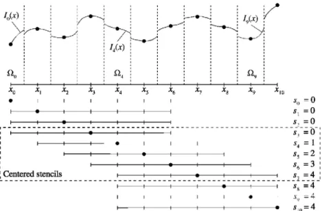
deriva-tives are then computed to obtain the sought finite difference for-mulas. Fig. 1 represents such a piecewise polynomial interpolant formed out of individual polynomial interpolants /,(x) which are only valid in their respective domains of validity f2,. Each of these domains f2, includes the corresponding grid node x, and their union is equal to the whole domain [-1,+1] of the problem.
Given a set of grid nodes, the expressions for/,(x) can readily be obtained through the Lagrange interpolation formulae [39,40]:
m = J2^ij{x)uj,
^«w-
n
J^f^
m = 0 ^' x„+„
Si + mj^i
(21)
where q is the polynomial degree and the seed s, is the index of the left most node x, involved in the construction of the interpolant /,(x). For the case of even polynomial degrees, which is the choice from now on, the following selection of values for s, is made:
{Si} = { 0 , . . . , 0 , 0 , 1 ,
g/2 times ce
,N-q,N-q,...,N-q}. (22)
g/2 times
; Centered stencils
s, = 0
s,=4 s,=4
Fig. 1. Stencils, seeds Si, and domains of validity Qi of the individual polynomial interpolants /i(x) of a piecewise polynomial interpolation of degree q = 6 on 11 nodes {N = 10). The dashed box separates the centered stencils from those affected by the presence of the boundaries.
the stencils are biased towards the center of the domain in order to only make use of existing grid nodes.
It should be noted, that in virtue of the uniqueness of the inter-polating polynomials, the finite difference formulas obtained from the differentiation of the piecewise polynomial interpolant intro-duced above coincide with the ones obtained by classical means. Thus, no differences compared to conventional finite difference methods on arbitrary grids exist, only the way in which they are formulated and derived, but not in the end result.
In the above definition of the piecewise polynomial interpolant the choice of grid nodes x, has been left open so far. However, by their proper selection it is possible to make the interpolation error of the piecewise polynomial interpolant to be uniform across the interval [-!,+!]. The result is a non-uniform grid that is unique for each pair of values of q and N. This same idea underlies the Chebyshev interpolation, where the condition that the interpola-tion error is uniform across the interval [-!,+!] is also imposed, but this time on a single polynomial interpolant instead [41,42]. The result is also a non-uniform grid, known as the Chebyshev roots or Chebyshev-Gauss quadrature points, that is unique for each value of N. Both approaches achieve the same result, namely the suppression of the Runge phenomenon that spoils the accuracy of high order polynomial interpolations close to the ends of the interpolation interval.
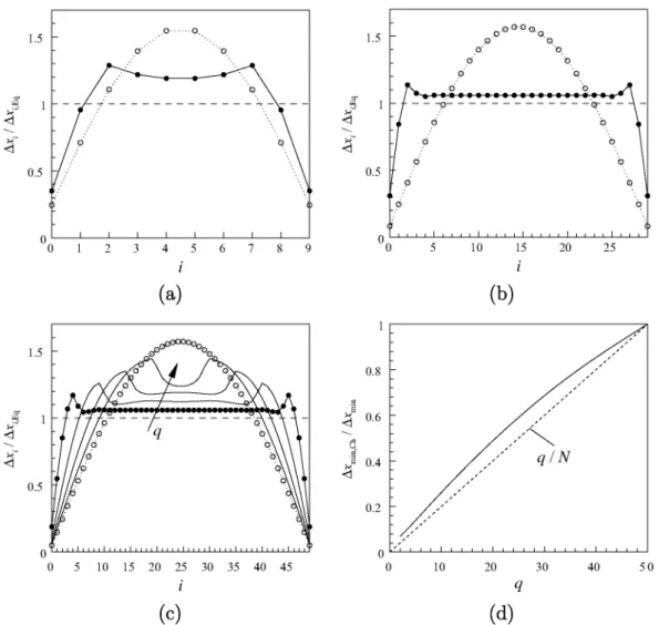
In Fig. 2 the resulting grid spacings Ax, = x,+] - x, for the piece-wise polynomial interpolant and for the Chebyshev interpolant are shown for different cases, both of them normalized with the uni-form grid spacing Ax, Eq = 2/N. The details of the algorithm for the derivation of the former one can be found in [32], while the derivation of the Chebyshev grids can be found in any classical textbook on spectral collocation methods or interpolation theory [40-42]. The case q = 6 and N = 10 from Fig. 1 is shown in Fig. 2(a), where it can be seen that the proposed non-uniform grid for the piecewise polynomial interpolant lies in between the uni-form grid and the Chebyshev grid.
Very enlightening are the following limiting cases: (i) q^N and (n) q = N. In the first case, only a few points 0{q) close to the boundaries need to be clustered in order to control the interpo-lation error, while far from the boundaries the grid points are equally spaced, as seen in Fig. 2(b), where the case of a piecewise polynomial interpolant for q = 6 and N = 30 is shown. In the
sec-ond case, when q =N, only one interpolating polynomial can be constructed out of the N + 1 grid nodes, thus /o(x)=/](x)
= • • • = /N(X). Due to the uniqueness of the interpolating
polynomials and the fact that the same error uniformization strat-egy is used for the piecewise polynomial interpolant than for the Chebyshev interpolant, both approaches are identical. Thus, in the limit q = N, the proposed piecewise polynomial interpolant with the proposed non-uniform grid presents all the properties of spectral collocation methods, especially their spectral accuracy [42-44].
When q < N, most of the nodes are affected by the presence of the boundaries and the resulting grid point distributions are in be-tween the two limiting cases. This can be seen in Fig. 2(c), where the grid spacing of the proposed non-uniform grids for different values of q and N = 50 are shown. As the degree of the interpola-tion increases, the node distribuinterpola-tion approaches the Chebyshev grid, while for small values of q it is more close to the uniform grid. Fig. 2(d) shows that the minimum grid spacing AXmin present in the proposed non-uniform grids is always greater than the minimum grid spacing AXminch of the Chebyshev grid. Moreover, from the fig-ure in can be inferred that AXmin = C'(AXmin,ch'V/l) = C'((qN)"M.
3.1.5. Spectral collocation methods
The limit of q = N in the FD-q methodology is the Chebyshev-Gauss-Lobatto spectral collocation method. The spectral methods offer an optimal compromise between the highest accuracy possible and the necessity of reducing the amount of information to be stored. The reason of the high accuracy of (collocation) spectral methods lies in the use of high-order interpolating polyno-mials, comprising all the points in the discretization domain. Spectral methods use all the points and the error is
e = 0{{1/Nf) -^0{e-^) [42,43]. Chebyshev-Gauss-Lobatto (CGL)
points:
Xj = cos(jn/N), j = 0,1, ,N, (23)
H I
(a)
(b)
(c)
(d)
Fig. 2. Grid spacing Axi = Xi+i - Xi of the non-uniform grid for the piecewise polynomial interpolation (solid line), for the Chebyshev interpolation (dotted line), and for the uniform grid (dashed line) normalized with the uniform grid spacing AXIE, = 2/N for (a) q = 6 and N = 10, (b) q = 6 and N = 30, and (c) q = 10,20,30,40 and N = 50. (d) Variation of AXmm,cii/AXmm with q of the non-uniform grid for the piecewise polynomial interpolation with N = 50.
3.2. Eigenvalue computation
The generalized eigenvalue problems must be constructed and solved employing adequate algorithms, taking into account the memory and CPU-time requirements when the matrices are formed and stored. Although the algorithm allows for the use of dense or sparse linear algebra, the sparse version is much more efficient and it is the one used here. The complex matrices A and
B of Eq. (4) are built using an in-house modified version of the
SPARSK1T2 library [45] to work with complex arithmetic. To solve the eigenvalue problem, the Arnoldi algorithm [46] is employed, combined with the MUMPS library [47,48] (MUltifrontal Massively Parallel Solver) to perform the LU-decomposition and solve the lin-ear algebraic systems with the possibility of making serial and par-allel computations.
The Arnoldi algorithm delivers a number of eigenvalues on the vicinity of a specific estimate value. Such value is set in the vicinity of the unstable/least-stable eigenvalue. Computational cost is greatly reduced when employing Arnoldi algorithm instead of the classical QZ method. More details can be found in the literature [46,21].
4. Results on the eigenvalue problem
In a linear modal framework, the overall behaviour of an unstable dynamical system is determined by its leading unstable
eigenvalues. Owing to the exponential growth of potential inaccu-racies in the eigenvalues, the major concern when performing fluid flow instability analyses is to capture in an accurate manner both the real and the imaginary parts of at least, the leading eigen-modes. This statement is true independently of the dimensionality of the base flow; however, on account of ambiguities in the base state determination, few global linear instability analyses are avail-able with sufficient quality to be used for validation of those deliv-ered by the spatial discretizations proposed herein.
In this respect, validations commence with the well-known Orr-Sommerfeld equation (OSE), to which the global eigenvalue prob-lem reduces in case of parallel flows. Results are presented for the plane Poiseuille flow (PPF) [49,50] and for the Blasius boundary layer [51].
Eigenvalue problems whose spatial dependence is described by the Poisson operator are subsequently solved by the present meth-odology, in both two and three spatial dimensions. The attractive-ness of this spatial operator resides in the existence of analytically-known results in regular two- and three-dimensional geometries and also in the fact that this spatial operator is at the heart of the global eigenvalue problem in both two and three spatial dimensions.
flow components: in the rectangular duct [6] only one such com-ponent exists, and the EVP is complex; in the 2D lid-driven cavity [52], two base flow velocity components exist, while the wave-number vector is normal to the base flow plane, and the stability eigenvalue problem is real; in the swept attachment-line boundary layer [53] all three base flow components exist and the eigenvalue problem is again complex. Finally, TriGlobal linear instability eigenvalue problems are solved, treating all three inhomogeneous spatial dimensions in a coupled manner. This is the most stringent test to which the proposed spatial discretization is employed. The same rectangular duct and 2D lid-driven cavity problems studied by BiGlobal analysis are solved by TriGlobal analysis. The solution is obtained at length-to-depth ratio of unity and a spanwise do-main extent defined by the maximally amplified BiGlobal eigen-mode, with which the TriGlobal analysis results are compared. It is worth noting that the very first TriGlobal instability analysis to appear in the literature was performed relatively recently in a time-stepping context [18], while presently four more such analy-ses are available [54,19,55,56]. Of these, one [54] is performed in a matrix-forming context, while two in a time-stepping technique, all concerning the cubic lid-driven cavity with singular lid motion [55,56].
4.1. Local instability analysis
The one-dimensional LNSE is the limit to which the global eigenvalue problem reduces in case of parallel flows. Results are presented for the plane Poiseuille flow (PPF) [49,50], the bounded nature of which implies the existence of a discrete eigenspectrum only, and for the Blasius boundary layer [51], where both discrete and continuous branches of the spectrum exist.
In order to assess the ability of the proposed spatial discretiza-tion to perform transient growth studies, the well-known pseudo-spectra of the OSE [57] are also obtained.
4.1.1. Eigenspectrum of plane Poiseuille flow
The temporal stability analysis of the plane Poiseuille flow is considered first. The stability eigenvalue problem [49] is solved at Re = 10000, a = 1 and spanwise wavenumber ^ = 0, for which the converged leading eigenvalue in double precision arithmetic has been provided by Kirchner [58] as being cOr.c + ic«i,c = 0.2375264888204682 + 10.0037396706229799. Owing to the relatively small leading matrix dimension, the dense linear algebra subroutine ZGGEV of LAPACK, based on the QZ algorithm [59], is used for the solution of the eigenvalue problem. The examined spatial discretizations are summarized in Table 1. All these finite difference methods are implemented at order 8 and on uniform grids, except for the last one, FD-q, which employs its particular grid. In addition, FD-q method is implemented not only at order 8, but also at order 16, in order to prove the capability of this method of reaching the resolution properties of very high order schemes. In Fig. 3, relative error of the leading eigenvalue as function of the leading matrix dimension N + 1 is presented in order to compare accuracy between the different numerical methods. The relative error is defined in the following way:
Table 1
Examined spatial discretization methods.
Spatial discretization method
Spectral collocation
Standard centered finite differences Compact finite-differences
Dispersion-Relation-Preserving finite differences Summation-by-parts operators
Finite difference methods with uniform error
Acronym
CGL STD Fade DRP SPB FD-q
References
[43,421 -1281 1291 [30,311 [321
0.01
0.0001
le-06
le-08
le-10
le-12
Fig. 3. Relative error for the amplification rate of the leading eigenmode of plane Poiseuille fiow at Re = W,a = 1 [49,501, obtained by (black) spectral collocation using CGL and (blue) high-order finite-difference methods of order 8: STD, Fade, DRP, SBP, as well as (red) FD-q with q = 8 and q = 16. N + 1 is the total number of discretization points. (For interpretation of the references to colour in this figure legend, the reader is referred to the web version of this article.)
CO,- - CO,v
ro,v (24)
where m, is the computed imaginary part of the eigenvalue using N + 1 nodes and m, c the corresponding converged value quoted above.
specified relative error level of 0(10 ^), or attaining an accuracy of 0(10"'°) for N = 200 points.
In summary, at all orders examined, the FD-q method performs better than all of the well-known high-order finite-difference methods. This is attributed to the fact that the FD-q method min-imizes the interpolation error both at the interior and the bound-ary (and near-boundbound-ary) points in a self-consistent uniform manner. In order for the standard high-order. Fade, DRP or SBP schemes to become competitive with FD-q, higher formal orders need to be used compared with that employed in the FD-q method. However, that increase in the order may not be straightforward for some schemes at q > 8 [30] or the resulting finite difference meth-od may be unstable.
On the other hand, for those methods for which using q > 8 is possible, the increase in bandwidth resulting from a comparatively high value of q is not an issue from the point of view of efficiency, when the one-dimensional eigenvalue problem is solved using full eigenspectrum computations and the QZ algorithm. However, FD-q has a competitive advantage in performing global instability anal-yses, where exploitation of the matrix sparsity is essential; there one seeks to use the method having optimal convergence and accu-racy properties between all available having the same sparsity pat-tern, as will be discussed in subsequent sections.
4.1.2. Pseudospectrum of plane Poiseuille flow
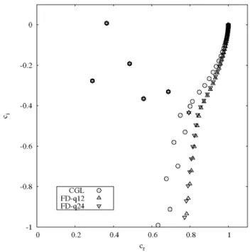
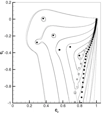
The non-modal scenario for laminar-turbulent flow transition is now well-understood [33], the concept of pseudospectrum [61] being central to its theoretical description. In this Subsection the pseudospectrum of plane Poiseuille flow (PPF) is shown compar-ing, for brevity, Chebyshev-Gauss-Lobatto collocation (CGL) and FD-ql6.
As in the previous Section, results obtained are representative of all combinations of number of discretization points, N, and finite-difference method order, q for FD-q; N = 128 and q = 16 are used presently, and the pseudospectrum has been computed using
Eig-Tool [62].
Fig. 4 shows the eigenspectrum and pseudospectrum obtained by the spectral collocation and finite-difference methods.
Eigenspectrum results are graphically indistinguishable from each other while the pseudospectrum, plotted here at different levels of matrix perturbations, corresponding to 10"' for the innermost to 10"^ in the outermost curve in Fig. 4, only shows discrepancies at large matrix perturbation levels. However, given that q ^ N, the overall agreement is quite satisfactory. If an improved agree-ment is sought, the order q or the number of points N may be in-creased in order for the FD-q method to deliver results approaching those obtained by the spectral collocation method. As mentioned, though, it is not perfect agreement of the FD-q with the spectral collocation method that is sought, but rather the abil-ity of the former method to deliver accurate description of the pseudospectrum, as shown in the results of Fig. 4, at a smaller cost thanks to the fact that q ^N, thus improving the sparsity pattern.
4.1.3. Eigenspectrum of the Blasius boundary layer
The accuracy properties of the FD-q method are preserved in open flows, where a mapping transformation is needed to transfer data from the standard domain x e [-1,1] of both the CGL and the FD-q methods onto a semi-infinite domainy e [0,y„]. The transfor-mation used is
y = L 1 -X 1 +s + x' L =
Vo^Vl
2y, s = 2L/y„ (25)
where y„ = 150 is the location where the calculation domain is truncated, with half the points being placed between the wall and y, = 5 [60].
Fig. 5 shows the leading unstable eigenmode and the least sta-ble part of the Blasius eigenspectrum at Res- = 580 and a = 0.179 [51], as recovered by the CGL spectral collocation method on N + 1 = 101 points, as well as FD-ql2 and FD-q24 on the same number of nodes. Even at a value of q which is an order of magni-tude smaller than N, the entire discrete eigenspectrum is seen to be recovered by the FD-q method as reliably as by the CGL spatial dis-cretization. None of the three methods is capable of capturing the continuous spectrum correctly; as is known analytically, the latter
Fig. 4. Eigenspectrum and pseudospectrum of plane Poiseuille flow at
i?e = 10'',a = l [49], obtained by spectral collocation using CGL and high-order flnite-difference method FD-q. Solid lines and empty circles: CGL, Dashed lines and solid circles: FD-ql6., both of them with N +1 =129 discretization points. Levels from inner to outer isoline, 10"^10"'^,10"^10"'',10"^,10"^ Note that c = m/a refers to phase velocity.
0
0.2
0.4
0.6
0.8
CGL FD-ql2 FD-q24
, 0
0
o A V
0
0
o 0
1
/ OS
O E
o *• m -a
^ ^
o
0 ^
° ^
^
A V
,
0.2 04 0.6 0.8
Fig. 5. Eigenspectrum of Blasius flow at Reg- = 580 and a = 0.179 [51], obtained
is a vertical line at Cr = cOr/a = 1 (c refers to phase velocity). Inter-estingly, even at q = 12 the discrete approximation of the continu-ous spectrum is more vertical than the one delivered by the spectral collocation method, although as q increases the FD-q and spectral results come closer, and collapse onto each other at
q = N, pointing towards the existence of an optimum value of q
which is unknown a priori. Finally, an additional discrete mode is recovered at Cr = 0.8 using the FD-ql2 and FD-q24 methods due to the displacement of the continuous part of the spectrum.
4.1.4. Pseudospectrum of the Blasius boundary layer
This Subsection of validation of results of the FD-q method against known solutions of the one-dimensional eigenvalue prob-lem closes with the presentation of the pseudospectrum of Blasius flow at the same parameters as those at which the eigenspectrum has been obtained. Fig. 6 presents the eigenspectrum obtained by the spectral collocation method, already shown in Fig. 5, alongside the one delivered by FD-ql6, which exhibits the properties dis-cussed in the previous Subsection. In addition, the pseudospectrum obtained at perturbation levels of 10"' to 10"^ (inner-to-outer curves) is shown. As in the case of the plane Poiseuille flow, close qualitative agreement is seen between the two sets of results, although the poor recovery of the continuous spectrum by both, the spectral and the finite-difference methods, results in larger dis-crepancies in the pseudospectrum in that region. By contrast, the pseudospectrum associated with the discrete eigenvalues is repro-duced in close agreement by both methods, despite the fact that q = 16 is an order of magnitude smaller than N + 1 = 129, the dis-cretization nodes used in both methods.
4.2. The 2D Helmholtz eigenvalue problem
In two spatial dimensions the Helmholtz eigenvalue problem (14) is:
= 0. (26)
6"0.4
-Fig. 6. Eigenspectrum and pseudospectrum of the Blasius boundary layer at
Rey =580 and a = 0.179 [51], obtained by spectral collocation using CGL and FD-q.
Solid lines and empty circles: CGL, Dashed lines and solid circles: FD-ql6, both of them with N + 1 = 129 discretization points. Levels from inner to outer isoline, 10"', 10"^ 10"^ 10"", 10"^ 10"^
Such problem is useful in assessing the accuracy of the proposed spatial discretization method comparing the recovered eigenvalues with the analytical solution of this problem in the rectangular membrane domain il = {x G [-1,1]} x {y G [-1,1]} [e.g. 34]. Such solution is the following:
l 2
•-^K + n'y); ,ny = 1,2,3, (27)
Higher eigenvalues/eigenfunctions ( n x , n y > l ) are of special interest due to the need of using a relatively high number of nodes for an accurate description. This is in contrast with the first few eigenvalues, which are already recovered using N R^ 10.
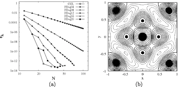
Fig. 7 shows the convergence history of the numerical solution of the 2D Helmholtz problem for a high eigenvalue (i^/(7r^/4) = 34) comparing the same finite difference methods used to obtain the OSE results in Fig. 3. Similar conclusions to the one reached in the Orr-Sommerfeld flow instability problem solved in the previous applications are also drawn here: maintain-ing the order of the scheme (order 8) FD-q presents higher accu-racy than the other finite difference methods, and with a higher order (order 16), FD-q reaches double-precision employing a num-ber of nodes only two times larger than employing the spectral col-location method.
Fig. 8(a) shows the convergence history of the numerical solu-tion of the 2D Helmholtz problem for the same eigenvalue. Differ-ent orders of FD-q methods are implemDiffer-ented and compared with CGL spectral collocation method. Special interest is focused on intermediate values of the order of the method, e.g. q = 12. In such case single-precision convergence is achieved using approximately two times more discretization points than with the spectral collo-cation method. In addition, double-precision convergence is achieved with less than four times more nodes than the ones re-quired by the spectral collocation method. For completeness.
le-06
le-08
le-10
N
Fig. 7. Convergence history of the solution of the 2D Helmholtz eigenvalue problem
>^ 0 -:
(b)
Fig. 8. (a) Convergence history of the solution of the 2D Helmholtz eigenvalue problem for the eigenvalue A^ /(ji^ /4) = 34, obtained using CGL and a suite of FD-q methods of
orders 4,8,12,16 and 20. The number of discretization nodes used is the same in both spatial directions and is denoted byN + 1. (b) Corresponding eigenfunction using FD-ql2 with Nx xNy = 80^. Shown are contours (-0.9:0.1:0.8) with isolines of positives (solid line) and negatives (dashed line) values.
Fig. 8(b) displays the eigenfunction corresponding to the eigen-value i^/(7r^/4) = 34, obtained numerically using FD-ql2 with
4.3. BiGlobal instability analysis
Attention is now turned to the main subject of this paper, namely modal global linear instability, discussing BiGlobal insta-bility first. Three applications are selected for validation purposes: the rectangular duct [6], the lid-driven cavity [52,63] and the swept leading-edge boundary layer [53,64]. As mentioned in the introduction to this section, these problems are selected because they are governed by one, two and three base flow velocity compo-nents, respectively, and also permit validating both the real and the complex form of the eigenvalue problem.
4.3.1. The rectangular duct flow
In two coupled spatial directions, the rectangular duct [6] of cross-sectional aspect ratio A, driven by a constant pressure gradi-ent along the axial (unbounded) direction, is the two-dimensional extension of the plane Poiseuille flow. Its base flow is known ana-lytically [65] and has a single component along the (homogeneous) wavenumber vector direction. Global flow instability in this appli-cation is governed by a complex eigenvalue problem.
Considering the rectangular duct defined in the domain
il = {x e [-A,A]} X {y e [-1,1]}, a constant pressure gradient in
the unbounded z direction drives a steady laminar flow which is independent of z and possesses a velocity vector U = [0,0, W(x,y)]^ with a single velocity component W{x,y) along the
z spatial direction. The latter satisfies the Poisson equation that
may be solved in series form [66].
Table 2 presents convergence history results for the numerical solution of the 2D EVP presented in Eq. (4) using the matrices (10) with base flow velocity U = [0,0,W(x,y)]'^, using CGL and FD-ql6 at a subcritical Reynolds number. Re = 1000, and wave-number parameter p = n.ln addition, Richardson-extrapolation re-sults are also shown. Considering the Richardson extrapolation value of CGL spectral collocation method as converged eigenvalue, 8 decimal digits are converged in cOr and 9 in co, when using CGL methods with N^ > 60^. On the other hand, the same order of con-vergence is reached when using FD-ql6 with N^ > 90^. Fig. 9
Table 2
Convergence history of BiGlobal instability analysis of rectangular duct flow at
A = ^,Re = 1000 and 11 = n comparing the leading eigenmode results using CGL and
FD-ql 6 and the corresponding Richardson extrapolations.
CGL
Richardson Ext. FD-ql6
Richardson Ext. N^
30^ 40^ 50^ 60^ 70^
30^ 50^ 70^ 90^
110^
Or
2.9027647730 2.9027654432 2.9027654495 2.9027654518 2.9027654528 2.9027654541 2.9027679758 2.9027654409 2.9027654496 2.9027654520 2.9027654529 2.9027654541
COi
-0.10353535398 -0.10352492808 -0.10352492616 -0.10352492608 -0.10352492609 -0.10352492635 -0.10352715467 -0.10352492446 -0.10352492422 -0.10352492512 -0.10352492555 -0.10352492637
shows the convergence history for the different spatial discretiza-tion schemes, using the converged result of Table 2, co = 2.9027654541 - iO.10352492635, as correct value. Different slopes arise due to the discontinuities of the derivatives in the cor-ners of the domain [43]. As expected, the convergence rate for FD-ql 6 and CGL are better than for the order 8 schemes. However, the higher degree of sparsity in the 8th-order scheme makes FD-q8 the more efficient one in terms of the numerical solution of the 2D EVP presented in Eq. (4) with the matrices (10).
4.3.2. The regularized lid-driven cavity
le-05
le-06
le-08
le-09
N
Fig. 9. Convergence history of the BiGlobal eigenvalue problem applied to the rectangular duct flow at i?e = 1000 and ll = n, with A = l for the eigenvalue 0 = 2.9027654541-10.10352492635, obtained by (balck) spectral collocation using CGL and (blue) high-order flnite-difference methods of order 8: STD, Fade, DRP, SBP, as well as (red) FD-q with q = 8 and q = 16. The number of discretization nodes used is the same in both spatial directions and is denoted by N + 1. (For interpretation of the references to colour in this flgure legend, the reader is referred to the web version of this article.)
0.001
le-05
le-06
20 50 100 200
N
Fig. 10. Convergence history of the BiGlobal eigenvalue problem applied to the regularized lid-driven cavity flow at Re = 1000 and yff = 15, with A = 1 for the most unstable eigenvalue m = 10.108337, obtained by (black) spectral collocation using CGL grid and (blue) high-order flnite-difference methods of order 8: STD, Fade, DRF, SBF, as well as (red) FD-q with q = 8 and q = 16. The number of discretization nodes used is the same in both spatial directions and is denoted by N + 1. (For interpretation of the references to colour in this flgure legend, the reader is referred to the web version of this article.)
The direction x is taken to be in the direction of the motion of the lid andy to be along the normal to this direction. The base flow is considered independent of the third (spanwise) direction z. Thus, the domain is defined as il = {x e [0,A]} x {y e [0,1]}, where A is the aspect ratio. The steady base flow vector under these assump-tions has two velocity components, U = [U{x,y), V(x,y), 0]^, and it is obtained by solving the vorticity-transport equation (see [21] for more details). The boundary conditions are V = 0 on all four walls and U = 0 in all the walls but the corresponding to the lid where
[ 7 = 1
• (2x-\y'f
X€ [0,1]. (28)In this manner, the discontinuity in the boundary condition at U(x = 0 , y = l ) and U(x = l,y = l) of the lid-driven-cavity flow [67,68] is avoided, since it is a potential source of suboptimal convergence.
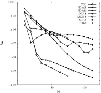
Fig. 10 presents convergence history results using the same suite of 8th-order finite difference methods used so far, in addition to FD-ql6 and CGL. At the conditions at which the eigenvalue prob-lem in Eq. (4) with the matrices (10) is solved, the leading eigen-mode is stationary, so comparisons are performed using only the imaginary part of the leading eigenvalue. The converged value used for this result is the average obtained while Richardson extrapola-tion of the CGL and FD-ql6 methods. The same qualitative conclu-sions reached by application of these discretization methods in the previous problems are reached here too, namely that the FD-q methods are superior in terms of accuracy to all other finite-differ-ence approaches.
It is worth noting in this context that the only previous known work in the literature which compares finite-difference and spec-tral collocation methods for global instability analysis is the work by Merle et al. [27] who also used the lid-driven cavity as test. The conclusion reached in that work was that the DRP scheme is the best alternative in terms of computational cost to CGL from a combined accuracy and efficiency perspective. This conclusion is
superseded by the results of Fig. 10: while the DRP method has the same formal resolution capacity as standard, Pade or SBP fi-nite-differences, and may indeed be more efficient than some of the other methods examined (comparisons in [27] were confined to Pade and DRP), the 8th-order member of the FD-q methods fam-ily significantly outperforms all its peers; using N = 100 it delivers a relative error of the most unstable eigenmode of ©(lO""*), as op-posed to 0(10"^) that all other finite-difference methods deliver. In addition, due to the nature of the method, the sparsity of DRP is smaller than the one of FD-q when the order of the method is the same in both numerical schemes. As in the previously studied problems, increasing the order of the FD-q method utilized delivers results approximating those obtained by the spectral collocation method.
4.3.3. The swept attachment-line boundary layer flow
Still within a BiGlobal context, the eigenvalue problem govern-ing instability of the incompressible swept Hiemenz flow is also solved using the proposed spatial discretization methods. Unlike the two previous two-dimensional base flows, here all three base flow velocity components are present and no reductions of the lin-earized Navier-Stokes equations are possible. Here too a complex eigenvalue problem needs to be solved. One advantage of this application is that the base flow is obtained by the solution of sys-tems of coupled ordinary differential equations at arbitrarily high precision. In addition, accurate global instability results of this flow are available [53] and have been modeled by simple one-dimen-sional eigenvalue problems in both the orthogonal [64], and the non-orthogonal [69] leading-edge boundary layer flow, providing highly accurate data to compare against.
Table 3
BiGlobal instability analysis of the incompressible swept attachment boundary layer flow with at Re = 800 and /J = 0.255. The first two most unstable modes, GH and Al are shown. Comparison with the results presented by Lin & Malik [53]. Note that c = 01/p refers to phase velocity.
N^ Cr(GH) Ci(GH)(xl02) CriAV) Ci(Al)(xlO^)
CGL
FD-ql6
FD-q8
L&M [531
30^ 40^ 50^ 60^ 30^ 50^ 70^ 90^ 30^ 50^ 70^ 90^
0.35840506 0.35841015 0.35840978 0.35840997 0.35842026 0.35840951 0.35840947 0.35840990 0.35840088 0.35841011 0.35840976 0.35840991 0.35840982
0.58473709 0.58531622 0.58532857 0.58531393 0.58484758 0.58533098 0.58529166 0.58532679 0.58685134 0.58540140 0.58530175 0.58532658 0.58532472
0.35791126 0.35792172 0.35792622 0.35792318 0.35792767 0.35791855 0.35791927 0.35791979 0.35790972 0.35797511 0.35791916 0.35791980 0.35791970
0.41108252 0.41104656 0.41027206 0.40962663 0.40974017 0.40989817 0.40986547 0.40988838 0.41179370 0.40990771 0.40989455 0.40988576 0.40988667
U{x,y) is taken to be linearly dependent on the chordwise
coordi-nate X, while the wall-normal velocity component V(y) and the velocity component W(y) along the attachment line are taken to be independent of x [65],
The eigenvalue problem in Eq. (4) with the matrices (10) is solved with this attachment line boundary layer base flow using the same set of parameters of [53]: Re = 800 and p = 0.255. The transformation used for the wall-normal direction y is the same as the one used for the Blasius boundary layer problem (25) but with y^ = 150 and Vi = 4. In the chordwise coordinate, a linear transformation is used to map the standard CGL or FD-q domain into x e [-200,200], Table 3 shows comparisons with the con-verged results of [53] using CGL, FD-q8 and FD-ql6 for the first two most unstable modes, FD-q8 and FD-ql6 results show very good agreement with the literature result and even outperform the CGL results of the second eigenvalue using low resolution (e,g, Nx X Ny = 50^), which is more difficult to be calculated numerically, due to the closeness between both modes.
4.4. The 3D Helmholtz eigenvalue problem
In three spatial dimensions the Helmholtz eigenvalue problem (14) is defined by the following equation:
9x2 0, (29)
Such problem is useful in assessing the accuracy of the proposed spatial discretization method, especially in the recovery of the high-er eigenvalues/eigenfunctions, nx,ny,nz » 1, The recovhigh-ered eigen-values are compared with the analytical solution of this problem in the domain Cl = {xe[-1,1]} x {y G [-1,1]} x {z e [-1,1]} [34], Such solution is the following:
-nl];
nx,nv,nz = 1,2,3, (30)Fig, 11(a) shows the convergence history of a high eigenvalue
(A'^/{TI^/4) =43), Conclusions analogous to those reached in the
two-dimensional Helmholtz eigenvalue problem and in the previ-ously addressed applications are also drawn here. Special interest is focused on intermediate values of the order of the method, e,g,
q = 12,q = 14. Single-precision convergence is achieved using
approximately two times more discretization points than with spectral collocation methods, and double-precision convergence is achieved with less than four times more nodes than with spec-tral collocation methods.
For completeness. Fig, 11(b) displays the eigenfunction corre-sponding to the eigenvalue (A'^/{TI^/4) = 43), obtained numerically using FD-ql2, showing that a non-trivial structure in terms of gra-dients is obtained. As with its two-dimensional analogue, reliable spatial discretization of the three-dimensional Poisson operator sets the scene for the solution of the TriGlobal eigenvalue problem,
4.5. The TriGlobal eigenvalue problem
Finally, the TriGlobal linear instability eigenvalue problem in Eq, (4) formed by the matrices (13) is solved, treating all three inhomogeneous spatial dimensions in a coupled manner.
Using the two-dimensional rectangular duct and regularized lid-driven cavity base states previously calculated, a three-dimen-sional, spanwise homogeneous base flow is constructed and
analyzed by solving the three-dimensional eigenvalue problem without exploitation of the spanwise periodicity. This is the most stringent test to which the proposed spatial discretization is ex-posed. In view of the results, only the FD-q method is used for the solution of Eq. (4) formed by the matrices (13).
4.5.1. The rectangular duct flow
The rectangular duct flow is analyzed also with TriGlobal anal-ysis at Re = 1000, employing FD-qlO in both x andy directions. For the TriGlobal analysis, Np Fourier collocation points are used along the spanwise direction, in order to discretize a spanwise length Lz = 2n/figQ. The parameter fi^Q = n'ls chosen to enable direct com-parisons of the present TriGlobal with the results obtained by the solution of the BiGlobal analysis in which only (x,y) are discretized in a coupled manner. Results are presented in Table 4, where a very good agreement between BiGlobal and TriGlobal analysis results is observed: the damping rate obtained by BiGlobal analysis using the highest attainable resolution on the used desktop computer,
Nx X Ny = 70^ CGL points and that delivered by the TriGlobal
anal-ysis with Nx X Ny = 56^ FD-qlO points and Nf = 12 Fourier colloca-tion points, have a relative difference of 0(10"').
4.5.2. The regularized lid-driven cavity
The last test to which FD-q methods are subject is the two-dimensional regularized lid-driven cavity flow analyzed with Tri-Global analysis. For the solution of Eq. (4) formed by the matrices (13), Nf Fourier collocation points are used along the spanwise direction, in order to discretize a spanwise length L^ = 2n/figQ, and FD-qlO in both of the x and y directions. The parameters
Re = 1000 and figQ = \5 are chosen in order to directly compare
the present TriGlobal results with the results obtained with the BiGlobal analysis of Section 4.3.2. The results are presented in Table 5, where an acceptable agreement between BiGlobal and TriGlobal analysis results is observed: the damping rate obtained
Table 4
TriGlobal instability analysis of t h e r e c t a n g u l a r d u c t flow in t h e d o m a i n n = { x e [ - 1 , 1 ] } x { y e [ - 1 , 1 ] } X { z e [ - 1 , 1 ] } a t te = 1000 using FD-qlO for x a n d y direction w i t h N + 1 p o i n t s a n d Fourier collocation w i t h Nf points in z. The c o n v e r g e d BiGlobal result for t h e s a m e set of p a r a m e t e r s (i.e. using /J = TT) is s h o w n in Table 2: co = 2 . 9 0 2 7 6 5 4 5 4 - 1 0 . 1 0 3 5 2 4 9 2 6 4 . Tm a n d TAR respectively refer to t i m e s p e n t in t h e LU d e c o m p o s i t i o n of t h e m a t r i x a n d t h e Arnoldi iteration. Note t h a t ^ refers to in-core w h i l e t h e rest of results a r e out-of-core calculations.
N^ XNF
32^ X 12 40^ X 12 48^ X 12 42^ X 16 56^ X 12
Or 2.90275822 2.90276481 2.90276539 2.90276510 2.90276545
COi
-0.103516753 -0.103523881 -0.103524652 -0.103524201 -0.103524809
M e m o r y (MB) 48621" 2980 4611 6253 6539
Tw (s) 3531" 1006 1735 3345 5247
TAR{S)
0.81"
8.8
16.4 19.0 20.6
Table 5
TriGlobal instability analysis of t h e regularized lid-driven cavity flow in t h e d o m a i n n = { x e [0,1]} X {y e [0,1]} x { z e [0,27r/15]} at i?e = 1000 using FD-qlO for x a n d y direction w i t h N + 1 p o i n t s a n d Fourier collocation w i t h Nf p o i n t s in z. The converged BiGlobal result for t h e s a m e s e t of p a r a m e t e r s (i.e. using /J = 15) is s h o w n in Fig. 10: £0 = 10.108337.
N^ xNf 32^ X 12 40^ X 12 48^ X 12 42^ X 16 56^ X 12
COi
0.102726 0.106135 0.106903 0.106538 0.106804
Memory (MB)
49201" 3226 4578 6061 6704
Tm(s) 377I" 1447 1819 3097 3947
TAR{S)
O.9I
8.8
15.8 16.5 25.4
by BiGlobal analysis using Nx x Ny = 70^ CGL points and the one delivered by TriGlobal analysis with Nx x Ny = 56^ FD-qlO points and Nf = 12 Fourier collocation points show a relative difference of 0(10"^). This discrepancy is expected to improve by increasing resolutions. The degree to which this is possible for the present state-of-the-art computations is discussed next.
5. The efficiency advantages of the FD-q method
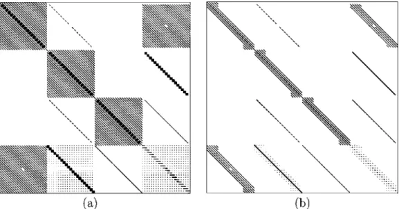
Once the accuracy of FD-q methods has been established, atten-tion may be turned to the efficiency advantage that they offer over spectral collocation methods. The solution algorithm is based on subspace iteration in which the spatial discretization matrix is formed, stored and LU-decomposed using sparse linear algebra routines and, therefore, the sparsity pattern is the key parameter for the success of the overall algorithm. Only the FD-q spatial dis-cretization has been monitored in terms of the memory and CPU time requirements for the serial solution of the incompressible BiGlobal EVP, on account of the superior accuracy properties of this over other finite-difference methods of the same formal order (and sparsity pattern). A visual indication of the savings expected by using a given FD-q method over the CGL spatial discretization is of-fered by the sparsity patterns resulting from spatial discretization of the left-hand-side BiGlobal matrix AID of Eq. (10), respectively shown in Fig. 12(a) for CGL and Fig. 12(b) for FD-q4, both plotted using N = 20. The key parameter when a sparse solver is used is the Number of Non-Zero elements (NNZ). For the differential oper-ators of this work, this parameter is reduced by a factor of
0{{q + 1)/(N+ 1)), with q the order of the used finite-difference
scheme (i.e. q + 1 is the stencil of the scheme) and N + 1, the num-ber of points used to discretize the problem in each spatial direc-tion for all the differentiadirec-tion matrices.^
The computational requirements of the overall numerical solu-tion of the EVP are imposed by those of the LU-decomposisolu-tion of the sparse matrix. The required memory and elapsed time for this factorization cannot be predicted a priori and the ratio ((q + 1)/(N+1)), elevated to a power to be determined later, is used next to relate the required memory and elapsed time of the LU-decomposition of FD-q with those of CGL spatial discretization. The flow instability problem chosen to study computational requirements is one in which all velocity components and their derivatives need to be discretized: the attachment line boundary layer (see Section 4.3.3). Spatial discretization methods used are the CGL discretization working in dense (results taken from [70]) and comparing them with the respective results corresponding to sparse CGL, FD-q8, FD-ql6 and FD-q24 spatial discretizations. For this problem, N = Nx = Ny, so the leading dimension of the matrix operator is M = 4 (N + 1 )^.
Table 6 shows the required memory for the LU decomposition of the BiGlobal EVP matrix using dense and sparse routines in con-junction with CGL discretization, as well as three members of the FD-q family and sparse linear algebra. The quantity of required memory when working in sparse is significantly reduced respect to the quantity of required memory working in dense, which is the-oretically Mem Ri 0{M^) R^ ©(N"*). The memory requirements of the FD-q8 method are found to be smaller by one order of magni-tude compared with those of the CGL method. In order to obtain a relation between the respective quantities the formula
Mem FD-q q + 1
N + 1 Memr (31)
' For t h e m o r e s t r i n g e n t case of c o m p r e s s i b l e BiGlobal instability analyses, or w h e n n o n - o r t h o g o n a l curvilinear m a p p i n g s a r e u s e d to discretize t h e p r o b l e m , cross-derivatives are p r e s e n t in t h e differential o p e r a t o r s . In this case, NNZ is r e d u c e d by a
Fig. 12. Sparsity pattern of the left-hand-side BiGlobal operator matrix with N +1 = 21 discretization points per spatial direction using (a) CGL and (b) FD-q4 in the
attachment line boundary layer problem, (blue) Real part and (red) imaginary part of the non-zero elements. (For interpretation of the references to colour in this figure legend, the reader is referred to the web version of this article.)
Table 6
Memory requirements for the LU decomposition (MB) in the attachment line boundary layer problem, using different resolutions and worldng with dense algebra for CGL and sparse algebra for CGL, FD-q24, FD-ql 6 and FD-q8. Note that N = N, = N,.
N
40 50 60 70
'-'-^1-dense
760
1747 3494 6230
"-•-JI-S parse
584
1350 3078 5544
FD-q24
444 705
1217 1889
FD-ql 6
246 457 775
1174
FD-q8
107 179 284 436
is assumed and used to identify (fit) tlie constant exponent a using tlie results of Table 6, plotted in Fig. 13(a). Independently both the CGL and the FD-q results are taken to follow a curve Mem oc (N +1)". This exponent is acGL = 4.1 for the sparse CGL method, which is very close to the theoretical exponent of 4 for dense computations, while the values 2.7,2.8 and 2.6 have been identified for FD-q24, FD-ql 6 and FD-q8, respectively. Using the average between the three FD-q cases, apo-q = 2.7, the constant exponent of Eq. (31) is approximated by a = ac ' F D - q = 1.4.
Fig. 13(b) shows the collapse of all FD-q curves using Eq. (31) and these constant values. The required memory for FD-q scales as MempD-q ~ 0{N^'') ~ ©(JW'^), which outperforms computations using CGL, the latter scaling as Memcci ~ 0{M^).
Turning to the elapsed time for serial LU factorization of the ma-trix pertinent to the same global stability EVP, results in Table 7 are presented for the same methods. The theoretical prediction of
0{M^) ~ 0{N^) is verified by the CGL either sparse or dense results.
The most striking result of this table is the order (s) of magnitude decrease of CPU time that the FD-q method offers, when compared with either of the CGL sparse or dense solution.
In order to quantify the relation between the elapsed times re-quired by the CGL and the FD-q methods, the formula
Time FD-q = 1
N + 1 ; Timer (32)
is assumed and used to fit the constant exponent b. Fig. 14(a) shows the results of Table 7. As in the case of memory requirements, either method is taken to follow a curve Time « (N-i-1)^. For the CGL
10000
o 1000
100
o
Pi
10000
1000