Malaria Cell Counting Diagnosis within Large Field of View
Li-hui Zou, Jie Chen, and Juan Zhang
Education Ministry Key Laboratory of Complex SystemIntelligent Control and Decision, School of Automation Beijing Institute of Technology
Beijing, China
{zoulihui, chenjie, zhjuan}@bit.edu.cn
Narciso García
Grupo de Tratamiento de Imágenes, E.T.S.I. Telecomunicación
Universidad Politécnica de Madrid Madrid, Spain
Abstract—Malaria is one of the most serious parasitic infections of human. The accurate and timely diagnosis of malaria infection is essential to control and cure the disease. Some image processing algorithms to automate the diagnosis of malaria on thin blood smears are developed, but the percentage of parasitaemia is often not as precise as manual count. One reason resulting in this error is ignoring the cells at the borders of images. In order to solve this problem, a kind of diagnosis scheme within large field of view (FOV) is proposed. It includes three steps. The first step is image mosaicing to obtain large FOV based on space-time manifolds. The second step is the segmentation of erythrocytes where an improved Hough Transform is used. The third step is the detection of nucleated components. At last, it is concluded that the counting accuracy of malaria infection within large FOV is finer than several regular FOVs.
Keywords-malaria diagnosis; cell counting; image mosaicing; Circle Hough Transform
I. INTRODUCTION
Malaria is one of the most common infectious diseases and an enormous public health problem. There were an estimated 190–311 million clinical episodes of malaria, and 708,000–1,003,000 deaths in 2008 [1]. It becomes the 5th cause of death from infectious diseases worldwide in low-income countries.
Malaria is caused by protozoan parasites of the genus Plasmodium. Four species of the plasmodium parasite infect humans, which are Plasmodium falciparum, Plasmodium vivax, Plasmodium ovale, and Plasmodium malariae. The most serious and virulent forms of the disease are caused by Plasmodium falciparum which contributes to the majority of deaths associated with the disease. Others only cause milder diseases in humans. Each malaria parasite life cycle can be divided into four stages which are merozoites, ring stage trophozoites, mature stage trophozoites, and then schizonts or gametocytes if sexual erythrocytic stages [2]. Rapid and accurate diagnosis facilitates prompt treatment, and it is an essential requirement to control malaria. The most economic, preferred, and reliable diagnosis is microscopic examination of blood films, especially the thin blood film examination which is the gold standard in diagnosis of malarial infection. Generally speaking, the diagnosis of malaria involves the following two or more tasks [3]:
• To determine the percentage of parasitaemia;
• To identify the species and the life-cycle stages of the detected parasites;
Usually, these jobs are taken by experienced microscopists manually. However, it is a time-consuming and tiring process that can be significantly affected by the expertise of the observer and, thus, have variable accuracy. Therefore, an automated image analysis system for accurate, fast and reliable determination of parasitemia is desirable.
Diagnosis of Malaria based on digital image analysis is totally a new research project started only in recent years [4]. Dealing with these two tasks above, blood smear image analysis has been tackled by using conventional image processing techniques like morphology, edge detection, region growing, thresholding, and pattern recognition techniques etc., which all have shown certain degrees of success with respect to the used sample images [5]. For example, a segmentation scheme for Red Blood Cells (RBCs) and parasites based on HSV color space was presented in [6] via detecting dominant hue range and calculating optimal saturation; in [7], the algorithm is based on edge detection and splitting large clumps made up from erythrocytes edge linking; in [8], it analyzes the infected blood cell images using morphological operators to segment cell images and to classify the parasites; F. B. Tek et al. proposed a novel binary parasite detection scheme that is based on a modified K nearest neighbor (KNN) classifier and compared three different classification schemes for the identification of the infecting species and life-cycle stages [9].
Here, in our research we mainly focus on the first task, determining the percentage of parasitaemia, because it is the most essential and time-consuming item in the diagnosis of malaria. The recommended procedure is by counting the numbers of parasitised red cells and all RBCs in a thin blood film and expressing the number of infected cells as a percentage of the RBCs. Some image processing algorithms to automate the diagnosis of this item on thin blood smears are developed, but the diagnosis results are sometimes higher than the manual counts as shown in the statistical results in [7]. One of the reasons is supposed to be that the cells at the borders of the images are often ignored. Besides, the statistic results in a single regular FOV can not reflect the global distribution of parasitaemia ratio due to the limitation of the amount of cells. In order to improve this statistical accuracy, a processing scheme within large FOV is proposed in this paper. The analysis process can be divided into three steps, 2010 Digital Image Computing: Techniques and Applications
image mosaicing, segmentation of erythrocytes, and detection of nucleated components. Particularly, in the first step, an optimal image mosaicing method which is based on space-time manifolds is presented to obtain large FOV. In the second step, an improved Hough Transform is used to segment the erythrocytes to get the whole number of RBCs. The third step is to detect the nucleated components mainly based on the basic difference between the blue and green channels. The work flow of our processing is shown in Fig. 1.
II. PROPOSED SCHEME
A. Acquisition of Large Field of View
A general image acquisition mode for obtaining large FOV is shown in Fig.2. There are parts of horizontal and vertical overlaps between neighboring images. Then a high-resolution mosaic with large FOV is obtained by image mosaicing technique. Considering the convenience for the operators, we recommend to shoot a video sequence with high-overlapped ratio between neighbor frames, which is also beneficial to create smooth mosaics. The original video sequence can be obtained through the trinocular biological microscope which can mount a video camera equipment to get digital images by moving the sample film smoothly along the travelling stage. The image acquisition system can be constructed under the simplest observation conditions without knowing explicitly the full motion or the calibration of the camera.
B. Image Mosaicing
Image mosaicing is an essential step for improving the counting precision in the proposed scheme. It can solve the the limitation of the FOV. The performance of image mosaicing algorithm will affect the following steps directly. In order to avoid additional introduced artifacts as much as possible, a smooth mosaic is required, not only smooth in color intensities, but also in geometric structure.
The research achievements in image mosaicing are fruitful during recent years [10]. Taking account of dense image capturing and the motion mode of the sample film in our application, the manifold-based image mosaicing technique [11] is more appropriate to solve the problems for video sequences under general motion conditions. A specific flow chart for image mosaicing is proposed in our scheme shown as Fig. 3. Since seldom motion and calibration information is known from an external device, we compute the motion parameters between neighboring frames and align the sequence by using phase correlation method. If great brightness differences caused by the auto-exposure or other natural factors exist among the neighboring images, they are eliminated by integrating with the motion estimation results to guarantee the smoothness in color intensities. And then the whole sequence whose brightness is already uniform is stitched into a high resolution image by using the space-time manifold-based mosaicing technique which utilizes the motion information among the frames more efficiently and ensures the smoothness in geometric structure of the synthetic mosaic.
• Motion estimation based on phase correlation
The efficient phase correlation method is used to determine the displacement (u, v) between two overlapped images. It is based on the translation property of the Fourier transform, that is, shifting a signal in time domain introduces linear phase difference in frequency domain.
Assume that there is a displacement (u, v) between image I1(x,y) and image I2(x,y), and I2(x,y) = I1(x-u,y-v). The Fourier
transforms of these two images, G1(ξ,η) and G2(ξ,η), satisfy
the following relationship:
2 ( )
2( , ) 1( , )
j u v
G ξ η =e− π ξ η+ G ξ η (1)
Hence the normalized cross-power spectrum of two images I1 and I2 with Fourier transform G1 and G2 is given
by:
*
2 ( )
1 2
1 2
( , ) ( , )
( , ) ( , )
j u v
G G
e
G G
π ξ η
ξ η ξ η
ξ η ξ η − +
× =
× (2)
Image Mosaicing
Segmentation of Erythrocytes
Nucleated Components Detection Motion Estimation
Mosaicing using Strips based on Space-Time Manifolds
Pre-processing for the Large Field of View Image
Hough Transformation for Multiple Circle Detection
Figure 1. Framework for malaria cell counting diagonis
Figure 2. A general image acquisition mode
Input Images
Motion Estimation based on Phase
Correlation
Eliminating the Brightness Difference
Figure 3. Image mosaicing approach for video sequence Space-Time Manifold-based
Mosaicing
where ‘*’ is the symbol of conjugation [12]. The translation property ensures the phase of the cross-power spectrum is equivalent to the phase difference between the images. The inverse Fourier transform of both sides of (2) can generate an impulse function δ at the point (u, v). Therefore, the displacement of these two images, (u, v), can be obtained by locating the peak of the inverse Fourier transform result. Additionally, if needed, the extended phase correlation method [13] can handle more general case, not only translation but also ration and scale between I1(x,y) and
I2(x,y).
One thing should be noted that other fast motion computation algorithms can be utilized too, as long as they can satisfy the demand of the processing efficiency, such as iterating Lucas-Kanade optical flow under Gaussian pyramid strategy for the motion estimation [14].
• Eliminating brightness differences
It is a preprocessing for the purpose of smoothing the color intensities for the mosaics. Firstly, adjacent frames are aligned by the motion estimation results. It is deemed that a step change in brightness is occurred around the current frame It if the average brightness difference ΔBt of the overlapped region between the current frame It and the
previous frame It-1 exceeds a threshold T. Then the current
frame It is taken as a brightness reference image Iref. The rule
can be described as follows:
, Bt ref t
if Δ ≥T then I =I (3)
(
)
1 1 1 1 1 1
( , ) t t ( , ) ( , )
Bt x ymeanI I I xt t u yt v It xt yt
− − − − − −
∀ ∈
Δ = ∩ + + − (4)
The color compensation can be conducted by adjusting (increasing or decreasing) all the previous or the following frames (depending on the position of the reference image in the whole sequence, if t<N/2, the previous, otherwise, the following) with the difference valueΔBt , i.e.
' 2, (1,..., )
2, ( ,..., )
i i Bt
if t N i t
I I
if t N i t N
< = ⎧
= + Δ ⎨
≥ =
⎩ (5)
It allows a brightness discontinuity between the adjusted image '
i
I and the reference image Iref no more than T. If
multiple brightness reference images are involved, the compensation can be handled iteratively until the global brightness difference under the threshold T.
• Space-time manifold-based mosaicing
The sprite of manifold-based mosaicing technique is inspired from line scaning using a 1D linear CCD camera whose imaging process can be modeled by a multi-perspective projection. They differ on the width and the shape of the scanning line. The ‘scanning line’ in manifold-based mosaicing is not just one single line, but several lines which are referred to as a strip. The shape of the strip is determined by the relative motion between the camera and the scanning scenes. In order to receive maximum information of the scanning scenes without missing or duplicating, the stripe requires being perpendicular to the
optical flow and its width should be proportional to the motion.
Optical flow can be interpreted as the motion between two neighboring frames taken at times t and t +δt at every pixel position. Due to the high-overlapped ratio among original images and the characteristic that seldom considerable depth differences are introduced, we can approximately take the motion estimation result above as the optical flow vector for every single point. Moreover, the relationship between neighboring images can be described by affine transform and expressed as:
1
1
t t t t
t t t t
x x a bx cy
u
y y d ex fy
v
−
−
− + +
⎛ ⎞ ⎛ ⎞
⎛ ⎞
=⎜ ⎟ ⎜= ⎟
⎜ ⎟ − + +
⎝ ⎠ ⎝ ⎠ ⎝ ⎠ (6)
where (xt-1, yt-1) and (xt, yt) are corresponding points in image
It-1 and image It, (u, v) is the optical flow vector as a function
of position (xn, yn), and (a, b, c, d, e, f) are the parameters of
the affine transform A. A cut line F(x,y)=0 which must be orthogonal to the optical flow (u, v) is calculated first. The normal line to F(x,y)=0 whose direction is
(
∂ ∂ ∂ ∂F x F x,)
, the same direction as (u, v), fulfills the request. This constraint can be expressed by:F
u a bx cy
x
k k
F v d ex fy
y
∂
⎛ ⎞
⎜∂ ⎟ ⎛ ⎞ ⎛ + + ⎞
⎜ ⎟= ⎜ ⎟= ⎜ ⎟
∂ + +
⎜ ⎟ ⎝ ⎠ ⎝ ⎠
⎜∂ ⎟
⎝ ⎠
(7)
The equation of the cut line is obtained if e = c:
2 2
0 ( , )
2 2 2
b c e f
F x y ax dy x + xy y M
= = + + + + + (8)
It is a family of lines that are all perpendicular to the optical flow, and M is used to select a specific line [15]. In our case, the relative movement between the sample film and the camera is smooth, only sideway translation or small vertical motion, the affine transformation A can take the form A=(a, 0, 0, d, 0, 0), thus the cut line becomes 0=F(x,y)=ax+dy+M whose slope is –a/d, and M is set to be the value for which the line contains maximum number of pixels in the center of the image where the distortions are minimum.
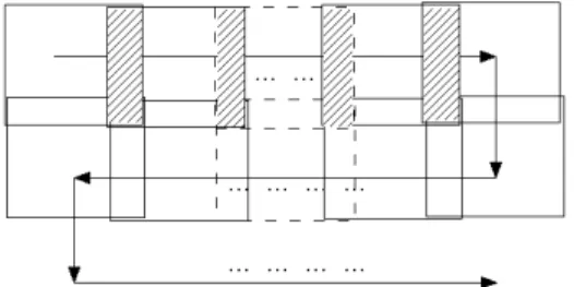
Narrow strips are selected from each image in the time domain to form the final space-time manifold. The schematic diagram of manifold-based image mosaicing approach is shown in Fig.4 [11]. Given the affine transformations At and
At+1, two cut lines ( , ) 0F x yt t t = and Ft+1(xt+1,yt+1) 0= can be
selected respectively. They are taken as the left sides of strips St and St+1. Furthermore, they determine the right sides
'
1 1
( , ) 0
t t t
F x− y− = and '
1( , ) 0
t t t
F+ x y = of their previous strips. For example, the right side '
1 1
( , ) 0
t t t
F x− y− = of strip St-1 is
computed by projecting the line ( , ) 0F x yt t t = onto the image It-1 using the transformation At. It makes the right side
of strip St-1 has the same properties as the left side of strip St
Figure 4. Schematic diagram of image mosaicing based on space-time manifolds
Mosaics
It-1 St-1 It St It+1 St+1
St-1St St+1
At At+1
Ft-1 Ft’ Ft F’t+1 Ft+1 F’t+2
side '
1( , ) 0
t t t
F+ x y = of strip St in image It, and the left side
1( 1, 1) 0
t t t
F+ x+ y+ = of strip St in image It+1 is associated by the
transformation At+1, etc. This selection of strips can keep the
orthogonality to the optical flow. And then these narrow strips from multiple images are cut out and warped together. The warping method is keeping the left side of each strip unchanged and warping the right side to match the left side of the next strip. It makes sure that each strip can be stitched seamlessly with the next strip. The width of each strip is proportional to the motion between the neighbor images. As a result, we can finally get a smooth and continuous mosaic after pasting all the warped cut strips.
C. Segmentation of Erythrocytes
The purpose of this step is to determine the denominator of the parasitaemia percentage, the whole number of RBCs in large FOV. An improved Circle Hough Transform (CHT) is used for detecting RBCs in consideration of the feature that blood cells belong to circular pattern. Compared with other segmentation algorithms for blood cells, CHT is one of the optimal selections for erythrocyte detection due to its efficiency and robustness. It can also handle the segmentation for the highly overlapping and oval cells [16].
Usually, the stained sample of thin blood film represents different performance in RGB color space. The RBCs are much more prominent in green channel than others. Therefore, we chose the green channel of the whole mosaics to segment the RBCs. The pre-processing, such as the enhancement of image contrast via adaptive histogram equalization, is necessary before CHT toreduce the effect of noises.
The CHT aims to find circular formations of a given radius R within an image by mapping the geometric space of images to the parameter space. A circle can be described by (9):
2 2 2
(x a− x) + −(y ay) =R (9)
where (ax, ay) are the coordinates of the circle center, and R
is the radius of the circle. An example of CHT is shown in Fig. 5 [17]. A set of edge points is indicated by the bold circle. Each edge point in the original image contributes a circle of radius R to the output parameter space, and this contribution is shown by these thin circles. These contributed
circles in parameter space intersect at the (ax, ay) as a peak
that is the center of the original circle in geometric space. The improved CHT for erythrocyte detection proceeds in the following steps [18]:
Step 1: Compute the gradient field of image intensity in green channel using the following equation:
(
)
( , )
( , ) ( , )
( , ) ( , 1), ( , ) ( 1, )
b x y i j
b b b b
I i j V V
I i j I i j I i j I i j
∇ =
= − − − − (10)
where ( , )∇I i jb is the gradient vector at pixel (i, j). And a thresholding on the gradient magnitude is performed before the voting process of CHT to remove the ‘uniform intensity’ image background.
Step 2: Convert the gradient field to an accumulation array where the pixel intensity corresponds to the probability of that pixel being the center of a RBC. The construction of the accumulation array which has same dimensions as the gradient field is done by a voting process in which the magnitude of∇I i jb( , ) is used as a weight value with a possible radius range of the RBCs.
Step 3: Detect the peaks in the accumulation array by a Laplacian of Gaussian (LoG) filter. The LoG filter can fill the transition areas between local peaks with negative values or zeros, which makes it easier to separate the peaks.
D. Nucleated Components Detection
This step is to determine the numerator of the parasitaemia percentage. Another observation among the color channels can be seen that in particular stained nucleated components result in distinctively high intensity values in the blue channel, while the same nucleated components in the green channel exhibit very low intensity values. Therefore, the differences between the blue Ib and the
green Ig color intensity channels are utilized to stretch the
contrast for visual perception and emphasize nucleated objects [5]:
{
}
,
min bg Ib Ig ∀x y Ib Ig
Δ = − − − (11)
If Δbg exceeds certain threshold, then mask it as a possible
nucleated component.
In order to identify the infected RBCs, the binary masks of nucleated component and the RBCs are used as follows. Since we can get every RBC mask which is separated with each other via the improved CHT, erode the RBC mask by applying a disk-shaped structural element of radius two to
obtain the inner region of the RBC where the nucleated components are possibly located. Then, the estimation of parasitemia for the separately occurring RBC can be accomplished straightforwardly by overlaying the binary masks of nucleated components and the RBC. Additionally, a cell is deemed to be infected if the area of its nucleated component masks exceeds a predefined threshold for removing the false positives.
III. EXPERIMENT RESULTS AND DISCUSSIONS In our experiments, to be concise, instead of the manipulation on a real image acquisition system, the video sequences were gathered from a simulated experiment platform shown in Fig. 6. It uses a projection screen to simulate the large FOV and a camera with a small FOV to get video sequences by moving along the screen. The camera path is parallel to the screen to simulate the motion mode of the real microscopic image acquisition system.
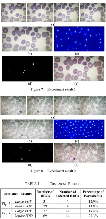
Two examples of malaria cell counting within the simulated large FOV are given to prove the validity of our philosophy. Fig. 7 (a) shows several original images from the video sequence, (b) is the image mosaicing result, (c) is the accumulation array in pseudo-color after CHT, (d) is the detection result of nucleated components, and (e) is the final detection result where the infected cells were marked with red ‘+’ at their center positions. Another example is shown in Fig. 8. And the counting results compared with regular FOVs are shown in Table 1. The statistic results of regular FOVs were computed by counting several original images with minimum overlapped areas separately and adding them together. It showed that the mosaicing results were satisfied and under the proposed scheme the counting accuracy within large FOV was finer than regular FOVs. The counting results of RBCs in large FOV were close to the true numbers, which shows that the improved CHT is an optimal algorithm for segmentation of erythrocytes. However, the method for detecting nucleated components was not so effective, see for example Fig. 8 where the detected infected cells were less than the true number due to the limitations of the acquisition process. In this kind of simulated experiment environment, the image quality decreased greatly due to the indirect imaging, especially affected by the uneven illumination as seen in Fig. 7(a) and Fig. 8(a) that the center areas of source images were brighter than the borders, which also made the brightness of generated mosaic images non-uniform. It brought difficulties for the analysis of the final mosaic image
as the original features in different color channels were changed, and led to the failure of nucleated component detection sometimes. Nevertheless, under the same detecting situation for nucleated components, it still can be seen that the statistical results of parasitemia percentage in large FOV were much more precise than those of several regular FOVs together.
As a matter of fact, there are various challenges to image analysis process in the practical microscopic malaria diagnosis system. Many inherent factors during the image acquisition process, such as different conditions of microscope components, different camera settings and so on, will influence the image quality. In addition, the differences in specimen preparation in terms of smearing, staining and Figure 6. Simulated experiment environment
(a)
(b) (c)
(d) (e) Figure 7. Experiment result 1
(a)
(b) (c)
(d) (e) Figure 8. Experiment result 2
TABLE I. COMPARING RESULTS
Statistical Results Number of RBCs Infected RBCsNumber of Percentage of Parasitemia
Fig. 7 Large FOV 31 4 12.9%
Regular FOVs 29 4 13.8%
Fig. 8 Large FOV 72 14 19.4%
cleanness will cause variations as often as the imaging conditions. All these factors can bring technical challenges to every step in the process scheme. Exposure difference and motion blur are main problems to image mosaicing. Dealing with the situation of cells overlap and cluster is the biggest challenge to the segmentation of erythrocytes, and the appearance of nucleated components can be affected by both imaging conditions and specimen preparations. Addressing these variations can contribute to the robustness of the system.
IV. CONCLUSIONS
There are many advantages of digital image analysis for helping the diagnosis of malaria. It can greatly liberate the microscopists from the manual time-consuming and tiring work. In our research work, one of the most important contributions must be highlighted is that we propose the scheme of malaria diagnose within large FOV. It can reduce the error of the total number of RBCs, which is caused by ignoring the cells at the borders of images, and improve the statistic accuracy for the percentage of parasitaemia. Imagine that the statistical cells are 10 or 100 times larger, the improved accuracy is appreciable. It makes image mosaicing become a meaningful work in the diagnosis of malaria.
ACKNOWLEDGMENT
This work is supported by Chinese National Science Fund for Distinguished Young Scholars, No. 60925011. Also, Li-hui Zou wishes to thank the Sino-Spanish Student Exchange Program of the Universidad Politécnica de Madrid for a personal research grant.
REFERENCES
[1] World Health Organization (WHO), “World Malaria Report 2009,” Geneva: WHO Press, 2009, available at: http://www.who.int/malaria/ world_malaria_report_2009/en/index.html.
[2] E. Ashley, R. McGready, S. Proux, and F. Nosten, “Malaria,” Travel Medicine and Infectious Disease, vol. 4, pp. 159-173, 2006.
[3] F. B. Tek, A. G. Dempster, and I. Kale, “Computer vision for microscopy diagnosis of malaria,” Malaria Journal 2009, 8:153 , 2009. [4] J. Frean, “Improving quantitation of malaria parasite burden with digital image analysis,” the Transactions of the Royal Society of Tropical Medicine and Hygiene, vol. 102, pp. 1062–1063, 2008.
[5] M-T Le, T. R. Bretschneider, C. Kuss, and P. R. Preiser. “A novel semi-automatic image processing approach to determine plasmodium falciparum parasitemia in giemsa-stained thin blood smears,” BMC Cell Biology, 9:15, 2008.
[6] V. V. Makkapati and R. M. Rao, “Segmentation of malaria parasites in peripheral blood smear images,” in Proceedings of the IEEE International Conference on Acoustics, Speech and Signal Processing, Taiwan, 2009, pp. 1361–1364.
[7] S. W. S. Sio, et al. “MalariaCount: an image analysis-based program for the accurate determination of parasitemia,” Journal of Microbiological Methods, vol. 68, pp. 11–18, 2007.
[8] C. D. Ruberto, A. Dempster, S. Khan, and B. Jarra, “Analysis of infected blood cell images using morphological operators,” Image and Vision Computing, vol. 20, pp. 133–146, 2002.
[9] F. B. Tek, A. G. Dempster, and I. Kale, “Parasite detection and identification for automated thin blood film malaria diagnosis,” Computer Vision and Image Understanding, vol. 114, pp. 21–32, 2010.
[10] R. Szeliski, “Image alignment and stitching: A tutorial,” Foundations and Trends® in Computer Graphics and Vision, vol. 2, pp. 1–104, 2006.
[11] S. Peleg, B. Rousso, A. Rav-Acha, and A. Zomet, “Mosaicing on adaptive manifolds,” IEEE Transactions on Pattern Analysis and Machine Intelligence,vol. 22, pp. 1144–1154, 2000.
[12] C. D. Kuglin and D. C. Hines, “The phase correlation image alignment method,” in Proceedings of the IEEE International Conference on Cybernetics and Society, New York, United States, 1975, pp. 163–165.
[13] B. S Reddy and B. N. Chatterji, “An FFT-based technique for translation, rotation, and scale-invariant image registration”, IEEE Transactions on Image Processing, vol. 5, no. 8: 1266–1271, 1996. [14] L-H Zou, J. Chen, J. Zhang and L-H Dou, “An image mosaicing
approach for video sequences based on space-time manifolds (in Chinese)” in Proceedings of the 29th Chinese Control Conference, Beijing, China, 2010, pp. 3003–3006.
[15] B. Rousso, S. Peleg, and I. Finci, “Mosaicing with generalized strips”. In DARPA Image Understanding Workshop, New Orleans, United States, 1997, pp. 255–260.
[16] R. Pinzón, G. Garavito, Y. Hata, L. Arteaga, and J. D. García, “Development of an automatic counting system for blood smears (in Spanish) ,” in Proceedings of the Congress of the Spanish Biomedical Engineering Society, 2004, pp. 45–49.
[17] T. J. Atherton and D. .J. Kerbyson, “Size invariant circle detection,” Image and Vision Computing, vol. 17, pp. 795–803, 1999.