In recent years, the study of artifi cial neural networks (ANN) have aroused great interest in fi elds as diverse as biology, psychology, medicine, economics, mathematics, statistics and computer science. The main reason underlying this interest lies in the fact that ANN are general, fl exible, nonlinear tools capable of approximating any sort of arbitrary function (Hornik, Stinchcombe, & White, 1989). Due to their fl exibility as function approximators, ANN are robust methods in tasks related with pattern classifi cation, the estimate of continuous variables and time series forecasting (Kaastra & Boyd, 1996). In this latter case, ANN offer several potential advantages with respect to alternative methods —mainly ARIMA time series models— when it comes to dealing with problems concerning nonlinear data which do not follow a normal distribution (Hansen, McDonald, & Nelson, 1999). The fi rst advantage lies in the fact that ANN are extremely versatile and do not require formal specifi cation of the model or the fulfi lment of a certain probability distribution for the data.
Regarding the second advantage, Masters (1995) shows that ANN are capable of tolerating the presence of chaotic components in better conditions than most alternative methods. This capacity is particularly important due to the fact that many of the relevant time series possess systematic chaotic components.
In this way, ANN have been successfully applied in time series forecasting in different knowledge fi elds such as biology, fi nance and economics, energy consumption, medicine, meteorology and tourism (Palmer, Montaño, & Franconetti, 2008).
The most widely used neural network in time series forecasting has been the MLP (Multilayer Perceptron) (Bishop, 1995). However, recent studies have evidenced the excellent performance of other neural network models with respect to the MLP model in this type of task (Liu & Quek, 2007). As far as ANN are concerned, the literature has not established a general procedure of application of this technique in time series forecasting, but rather aspects in which there is no agreement between several authors have been presented (Nelson, Hill, Remus, & O’Connor, 1999). In this sense, this study offers a description and a comparison of the main ANN models that have been shown to be useful in time series forecasting, as well as a standard procedure for the practical application of ANN in this type of task. The models analyzed are: the Multilayer Perceptron (MLP), Radial Basis Function (RBF), Generalized Regression Neural Network (GRNN) and Recurrent Neural Networks (RNN).
Fecha recepción: 21-6-10 • Fecha aceptación: 1-12-10 Correspondencia: Juan José Montaño Moreno Facultad de Psicología
Universidad de las Islas Baleares 07122 Palma (Spain) e-mail: [email protected]
Arti
fi
cial neural networks applied to forecasting time series
Juan José Montaño Moreno
1, Alfonso Palmer Pol
1and Pilar Muñoz Gracia
21 Universidad de las Islas Baleares and 2 Universidad Politécnica de Cataluña
This study offers a description and comparison of the main models of Artifi cial Neural Networks
(ANN) which have proved to be useful in time series forecasting, and also a standard procedure for the practical application of ANN in this type of task. The Multilayer Perceptron (MLP), Radial Base Function (RBF), Generalized Regression Neural Network (GRNN), and Recurrent Neural Network (RNN) models are analyzed. With this aim in mind, we use a time series made up of 244 time points. A comparative study establishes that the error made by the four neural network models analyzed is less than 10%. In accordance with the interpretation criteria of this performance, it can be concluded that
the neural network models show a close fi t regarding their forecasting capacity. The model with the best
performance is the RBF, followed by the RNN and MLP. The GRNN model is the one with the worst performance. Finally, we analyze the advantages and limitations of ANN, the possible solutions to these limitations, and provide an orientation towards future research.
Redes neuronales artifi ciales aplicadas a la previsión de series temporales. El presente estudio ofrece
una descripción y una comparación de los principales modelos de Redes Neuronales Artifi ciales (RNA)
Method
Data
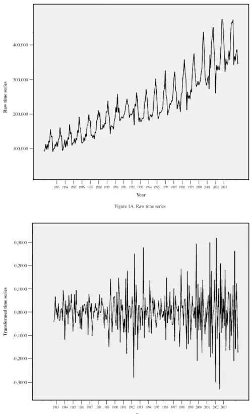
In this study we used the data concerning the total monthly electrical energy consumption (MWh unit) in the Balearic Islands between January 1983 and April 2003, obtaining a time series made up of 244 time points (from x1 to x244). In this sense, the forecast of electrical consumption constitutes one of the most paradigmatic problems in the fi eld of time series analysis (Pao, 2006).
Figure 1A shows the graphical representation of the original time series. A marked seasonal nature and an increasing linear trend can be observed. A review of the literature shows there is no agreement as to the need to eliminate the systematic components in time series when ANN are applied. Thus, some authors suggest ANN can adequately adjust both seasonality and the linear trend of a time series, based on the fact that ANN are capable of modelling any arbitrary function (Franses & Draisma, 1995). Other authors claim that despite being universal function approximators, ANN can benefi t from the previous elimination of systematic components, thereby focusing on learning the most complex aspects of the series (Nelson, Hill, Remus, & O’Connor, 1999). More recent empirical studies (Palmer, Montaño, & Sesé, 2006) show that the predictive performance of ANN improves if the systematic components have been previously eliminated from the time series.
In this way, following the traditional procedures of preprocessing time series, a logarithmic transformation was applied and two differentiations, one of order 1 and the other of order 12. Figure 1B shows the time series after applying these transformations.
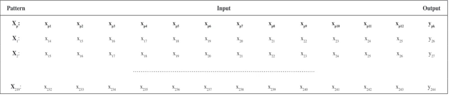
Modelling a univariate time series using ANN is generally carried out using a certain number of lagged terms in the series as the input and the forecasts as the output (Bishop, 1995). Following the methodology established by Masters (1993) as to the application of ANN in time series and bearing in mind that the data analyzed are monthly, for this study we carried out a forecast of each time point from the 12 lagged terms that would make up the previous year. Therefore, all the ANN models designed in this study are characterised by having 12 input neurons and one output neuron. After applying the transformations and the outline given in Figure 2, we found 219 input-output patterns (each one with 12 input values and one output value).
Then, the set of patterns was divided into three groups. The training group, made up of the fi rst 147 patterns; the validation group, made up of the following 36 patterns; and the test group, made up of the last 36 patterns.
Multilayer perceptron
A Multilayer Perceptron or MLP model is made up of a layer
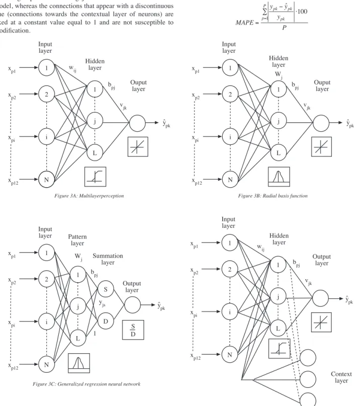
N of input neurons, a layer M of output neurons and one or more hidden layers; although it has been shown that for most problems it would be enough to have only one layer L of hidden neurons (Hornik, Stinchcombe, & White, 1989) (see Figure 3A). In this type of framework, the connections between neurons always feed forwards, that is, the connections feed from the neurons in a certain layer towards the neurons in the next layer.
The mathematical representation of the function applied by the hidden neurons in order to obtain an output value bpj, when faced
with the presentation of an input vector or pattern Xp: xp1, …, xpi, …, xpN, is defi ned by:
(1) where fL is the activation function of hidden neurons L, θj is the
threshold of hidden neuron j, wij is the weight of the connection between input neuron i and hidden neuron j and, fi nally, xpi is the input signal received by input neuron i for pattern p.
As far as the output of the output neurons is concerned, it is obtained in a similar way as the neurons in the hidden layer, using:
ˆypk= fM θk+ vjk⋅bpj j=1
L
∑ ⎛ ⎝
⎜ ⎞
⎠ ⎟
(2) where yˆpk is the output signal provided by output neuron k for pattern p, fM is the activation function of output neurons M, θk is the threshold of output neuron k and, fi nally, vjk is the weight of the connection between hidden neuron j and output neuron k.
In a general way, a sigmoid function is used in the hidden layer neurons in order to give the neural network the capacity of learning possible nonlinear functions, whereas the linear function is used in the output neuron in the event of an estimation of a continuous variable.
MLP network training is of the supervised type and can be carried out using the application of the classical gradient descent algorithm (Rumelhart, Hinton, & Williams, 1986) or using a nonlinear optimization algorithm which, as in the case of the conjugated gradients algorithm (Battiti, 1992), makes it possible to considerably accelerate the convergence speed of the weights with respect to the gradient descent algorithm.
Radial Basis Functions
Radial Basis Functions or RBF models (Broomhead & Lowe, 1988) are made up of three layers just like the MLP network (see Figure 3B). The peculiarity of RBF lies in the fact that the hidden neurons operate on the basis of the Euclidean distance that separates the input vector Xp from the weights vector Wj which is stored by each one (the so-called centroid), a quantity to which a Gaussian radial function is applied, in a similar way to the kernel functions in the kernel regression model (Bishop, 1995).
Out of the most widely used radial functions (gaussian, quadratic, inverse quadratic, spline), in this study the gaussian was applied as the activation function of the hidden neurons on input vector Xp, in order to obtain an output value bpj:
bpj=exp
xpi–wij
(
)
i=1
N
∑
2
2σ2 –
[
]
(3)If input vector Xp coincides with the centroid Wj of neuron j, this
The normalization parameter σ (or scale factor) measures the Gaussian width, and would equal the radius of infl uence of the neuron in the space of the inputs; the greater σ, the larger the region dominated by the neuron around the centroid.
The output of the output neurons is obtained as a linear combination of the activation values of the hidden neurons weighted by the weights that connect both layers in the same way as the mathematical expression associated with an ADALINE network (Widrow & Hoff, 1960):
Raw time series
100,000 200,000 300,000 400,000
1983 1984 1985 1986 1987 1988 1989 1990 1991 1992 1993 1994 1995 1996 1997 1998 1999 2000 2001 2002 2003
Year
Figure 1A. Raw time series
1983 1984 1985 1986 1987 1988 1989 1990 1991 1992 1993 1994 1995 1996 1997 1998 1999 2000 2001 2002 2003
Year -0,3000
-0,2000 -0,1000 0,0000 0,1000 0,2000 0,3000
T
ransformed time series
Figure 1B. Transformed time series
(4) Like the MLP network, RBF make it possible to carry out modelling of arbitrary nonlinear systems relatively easily and they also constitute universal function approximators (Hartman, Keeler, & Kowalski, 1990), with the particularity that the time required for their training is usually much more reduced. This is mainly due to the fact that RBF networks constitute a hybrid network model, as they incorporate supervised or non supervised learning in two different phases. In the fi rst phase, the weight vectors or centroids associated with the hidden neurons are obtained using non supervised learning through the k-means algorithm. In the second phase, the connection weights between the hidden neurons and the output ones are obtained using supervised learning through the delta rule of Widrow-Hoff (1960).
Generalized Regression Neural Network
The Generalized Regression Neural Network or GRNN (Specht, 1991) is made up of four layers of neurons: input layer, pattern layer, summation layer and output layer (see Figure 3C). As in the rest of the models described, the number of input neurons depends on the number of predictor variables established. This fi rst layer is connected to the second, the pattern layer, where each neuron represents a training pattern Xj and its output is a measure of the distance of the input pattern from each of the stored training patterns. Each neuron in the pattern layer is connected with each of the two neurons in the summation layer: the S-summation neuron and the D-summation neuron. The S-summation neuron calculates the sum of the weighted outputs in the pattern layer, whereas the D-summation neuron calculates the non-weighted outputs of the pattern layer. The weight of the connection between neuron j of the pattern layer and the S-summation neuron is yjs, the desired output
value corresponding to training pattern Xj. For the D-summation neuron, the weight of the connection is the unit. The output layer simply divides the output of the S-summation neuron by the output of the D-summation neuron, giving the prediction value for an input vector or pattern Xp: xp1, …, xpi, …, xpN, using the following expression:
(5)
where yˆpk is the output signal provided by output neuron k for input pattern Xp, bpj is the output signal of hidden neuron j after applying
a radial function in the same way as in expression (3) and yjs is the desired output of output neuron k for training pattern Xj.
The GRNN model allows us to carry out an estimate of the joint probability density function f(x, y) between a set of predictor variables x and a set of response variables y. This is closely related to the RBF network model and, just like this one, is based on kernel regression models. The main advantage of the GRNN model with respect to the MLP model is that it does not require an iterative training process. What is more, it can approximate any arbitrary function just like the previous models described, by adjusting the function directly from the training data.
Recurrent neural networks
Recurrent neural networks or RNN are especially useful in situations in which it is desired to represent the time relationships that may be established between the inputs and outputs of the neural network (Elman, 1990). In this type of network one layer of neurons possesses recurrent connections, that is, the outputs of the neurons are temporarily stored and then sent as input signals to the same neurons or to other neurons in the neural network. This process is represented in Figure 4.
The time delay operator Z-1 makes it possible to store the
output signals y obtained in the previous moments n of neuron j. In this way, a short term memory of the previous activation values generated by the neuron is generated. As far as the time parameter μ is concerned, it determines the weight or trace memory of the previous output signals y of neuron j. Thus, the output of neuron
j is a function of the input signals xi of neurons N in the layer immediately before and of the previous output signals y of this same neuron j weighted by the time parameter. The print or trace memory of the previous output signals decreases exponentially:
(6) where 0 < μ < 1
Recurrent neural networks, just like the previous models, possess a framework similar to an MLP model where one of the neural layers has recurrent connections. In this study we used the Elman network (Elman, 1990) in which the neurons in the hidden layer show recurrent connections. By this means, the neurons in this layer receive signals from themselves from previous moments and signals from the neurons in the input layer. As Jehee & Lee
Pattern Input Output
Xp: xp1 xp2 xp3 xp4 xp5 xp6 xp7 xp8 xp9 xp10 xp11 xp12 ypk
X1: x14 x15 x16 x17 x18 x19 x20 x21 x22 x23 x24 x25 y26
X2: x15 x16 x17 x18 x19 x20 x21 x22 x23 x24 x25 x26 y27
………
X219: x232 x233 x234 x235 x236 x237 x238 x239 x240 x241 x242 x243 y244
(1996) point out, this type of recurrence is especially useful for their application in time series forecasting. The recurrent connections stored by the lagged signals of the neurons are usually represented by a special layer of neurons called the context layer of neurons (see Figure 3D).
Concerning training this type of neural network, the connections that appear in the fi gure with a continuous line are modifi ed following supervised learning just as in the case of the MLP model, whereas the connections that appear with a discontinuous line (connections towards the contextual layer of neurons) are fi xed at a constant value equal to 1 and are not susceptible to modifi cation.
Measure of fi t
The most widely used measure of fi t in the fi eld of time series forecasting is the Mean Absolute Percentage Error (or MAPE) due to the fact that it is easy to interpret —it is interpreted in terms of percentage error— and does not depend on the measure scale of the variable (Witt & Witt, 1992):
(7)
1
2 1
i
N
L j xp1
xp2
xpi
xp12
Input layer
Hidden layer
Ouput layer bpj
vjk
yˆpk 1
L j Hidden
layer
Ouput layer wij
bpj
vjk
yˆpk 1
2
i xp1
xp2
xpi
xp12
Input layer
N
1
2
i xp1
xp2
xpi
xp12
Input layer
N
1
L j
D S Wj
bpj
yjs yˆ
pk
Pattern layer
Summation layer
Output layer
D S
1
2
i xp1
xp2
xpi
xp12
Input layer
N
1
L j wij
bpj
yˆpk Hidden
layer
Output layer vjk
Context layer
Figure 3A: Multilayerperception Figure 3B: Radial basis function
Figure 3C: Generalized regression neural network
Figure 3D: Elman recurrent network
Wj
1
where ypk is the desired value for output neuron k belonging to pattern p, yˆpk is the output signal of output neuron k for pattern p
and P is the number of total patterns analyzed.
Nevertheless, the distribution of the percentage errors is found limited between 0 and +∞; and in most cases this distribution has anomalous values or outlier values that are skewed to the right, leading to asymmetries (Smith & Sincich, 1988). As far as the MAPE is concerned, it does not constitute a resistant location index as it is based on the calculation of the arithmetic mean of the percentage errors and, therefore, is sensitive to the presence of outlier values.
With the purpose of overcoming the limitations presented by the MAPE as a measure of fi t in time series forecasting, in this study not only did we calculate the arithmetic mean of the distribution of the percentage errors, but we also obtained a resistant location index, the M-estimator of Huber (Huber, 1975).
Designed neural network models
In accordance with the description made, a set of MLP, RBF, GRNN and RNN network models were designed, from the manipulation of a series of parameters. In the case of the MLP models, different seed values were used for the initialization of the weights, as well as a number (between one and 4) of hidden neurons. The learning algorithm used was the conjugated gradients one (Battiti, 1992) and as an activation function of the hidden and output neurons, the sigmoid and linear ones, respectively. As far as the different RBF models are concerned, they were constructed by varying the number of centroids, between 5 and 25, and the value of the normalization parameter, between 0.2 and 1.5. In the case of the GRNN models, the only parameter that was manipulated was the normalization parameter with values comprising between 0.05 and 1. Finally, the RNN models, with recurrent connections in the hidden layer, were constructed by manipulating the same parameters as in the case of the MLP models.
For each of the four types of network model designed, the one that showed the lowest mean percentage error (MAPE, calculated using the M-estimator of Huber) with the validation group, was chosen.
Results
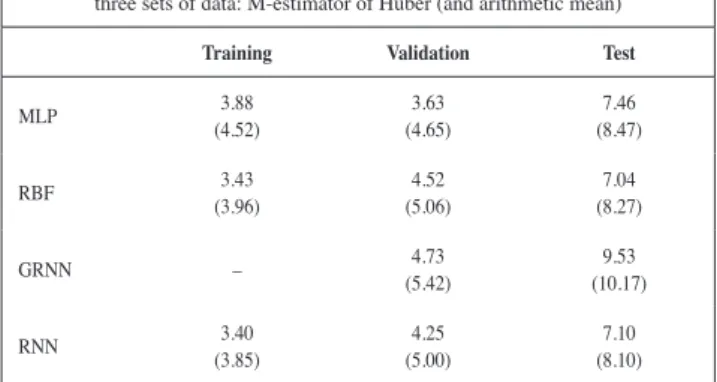
Table 1 shows the mean percentage error calculated using the M-estimator of Huber for each of the models selected in the validation phase, for the three sets of data. The value of the corresponding arithmetical mean appears in parenthesis.
It can be seen that the generalization error committed by each of the four network models analyzed and estimated from the test set, is less than 10%. In accordance with the interpretation criteria for the MAPE value established by Lewis (1982), the four neural network models can be considered to have highly accurate forecasting. The model with the best performance with the test group is the RBF, followed by the RNN and MLP. The GRNN model is the one with the worst performance with a difference of 2.49% compared to the model with the best performance, the RBF.
As far as the distribution of errors is concerned, it has been seen that in most cases they have outlier values, which is why the arithmetic means always provides a higher value than the M-estimator value.
Discussion
ANN can be considered general, fl exible, nonlinear statistical techniques capable of learning complex relationships between variables in a multitude of fi elds of study. This technique has a series of advantages compared to classical statistical models. First of all, ANN do not depend on the fulfi lment of statistical assumptions such as, for instance, the type of relationship between variables or the type of data distribution. Secondly, as universal function approximators, they are capable of fi tting linear and nonlinear functions without the need for knowing the shape of the underlying function a priori.
With respect to the limitations and criticisms received, ANN lack a theoretical foundation and a systematic procedure for the construction of the model, comparable to the classical approximations such as the Box-Jenkins methodology (Box & Jenkins, 1976). As a result, the construction phase of the model involves the experimental selection of a wide number of parameters by trial and error. The use of classical statistical procedures to determine the parameters of a neural network in time series forecasting could be useful in order to overcome this limitation (Hansen, McDonald, & Nelson, 1999). Nevertheless, the most criticised aspect in the use of ANN focuses on the study of the effect and signifi cance of the input variables of the model, due to the fact that the value of the parameters obtained by the network does not possess a practical interpretation, unlike classical statistical models. As a consequence, ANN have been presented to the user as a ‘black box’ as it is not possible to analyze the role played by each of the input variables in the forecast carried out. However, in recent years, different methods aimed at interpreting
Time parameter
Time delay operator x1
xN
x2 y
μ
Z-1
Figure 4. Artifi cial neuron with a recurrent connection
Table 1
Percentage error for each of the models selected in the validation phase for the three sets of data: M-estimator of Huber (and arithmetic mean)
Training Validation Test
MLP 3.88
(4.52)
3.63 (4.65)
7.46 (8.47)
RBF 3.43
(3.96)
4.52 (5.06)
7.04 (8.27)
GRNN – 4.73
(5.42)
9.53 (10.17)
the learning carried out by an ANN have been proposed. Most of these procedures are included in the so-called sensitivity analysis and have been applied satisfactorily in several fi elds of knowledge (Montaño & Palmer, 2003).
Among its contributions, this study has offered a description of the main ANN models aimed at time series forecasting. This line of research is clearly lacking, judging by the number of studies published in the context of Psychology (Palmer, Montaño, & Franconetti, 2008) in comparison with other types of application of this technique in fi elds such as, for instance, the classifi cation and prediction of patterns (Pitarque, Ruiz, & Roy, 2000), the imputation of missing data (Navarro & Losilla, 2000) or survival analysis (Palmer & Montaño, 2002).
This work aims to suggest that in all the fi elds of Psychology where classical time series models have been applied, ANN models could also be applied in a satisfactory way. By way of illustration, the fi elds of application could be about the use and abuse of psychoactive substances (Sears, Davis, Guydish, & Gleghorn, 2009), psychophysiological activity (Janjarasjitt, Scher, & Loparo, 2008), criminal or violent behaviour (Pridemore & Chamlin, 2006), assessment of psychological intervention programmes (Tschacher & Ramseyer, 2009), teaching methodologies (Escudero & Vallejo, 2000) or psychopathology (Valiyeva, Herrmann, Rochon, Gill, & Anderson, 2008).
Concerning the procedure proposed for the application of ANN in time series forecasting, we show the convenience, against the opinion of some authors, of carrying out preprocessing of the time series so as to eliminate the systematic components in them. Besides, we propose an improvement of the most widely used performance index to assess time series forecasting models, MAPE (Witt & Witt, 1992), through the calculation of an M-estimator rather than the arithmetic mean.
With respect to the overall performance of the four models analyzed, it is clear that ANN are fl exible, effective tools for all researchers interested in modelling the behaviour of time series. As far as the comparison between the models is concerned, the RBF, RNN and MLP models obtained the best results, whereas the GRNN networks obtained the worst results. This result could be due to the high dependency of the GRNN model as far as the training data selected are concerned.
Future lines of research should be aimed at overcoming the limitations mentioned in relation to the use of ANN, that is, the selection of the parameters related with the construction of the model and the analysis of the effect or signifi cance of the input variables in the forecast carried out. This work points out some possible directions to move in as far as this is concerned. Finally, it is also necessary to apply ANN to other databases in order to fi nd out the degree of generalization of the results obtained in this study.
References
Battiti, R. (1992). First and second order methods for learning: Between
steepest descent and Newton’s method. Neural Computation, 4,
141-166.
Bishop, C.M. (1995). Neural networks for pattern recognition. Oxford:
Oxford University Press.
Box, G.E.P., & Jenkins, G.M. (1976). Time series analysis: Forecasting
and control. San Francisco: Holden Day.
Broomhead, D.S., & Lowe, D. (1988). Multivariable functional interpolation
and adaptive networks. Complex Systems, 2, 321-355.
Elman, J.L. (1990). Finding structure in time. Cognitive Science, 14,
179-211.
Escudero, J.R., & Vallejo, G. (2000). Aplicación del diseño de series temporales múltiples a un caso de intervención en dos clases de
Enseñanza General Básica. Psicothema, 12, 203-210.
Franses, P.H., & Draisma, G. (1995). Recognizing changing seasonal
patterns using artificial neural networks. Rotterdam: Erasmus University Rotterdam.
Hansen, J.V., McDonald, J.B., & Nelson, R.D. (1999). Time series prediction with genetic-algorithm designed neural networks: An
empirical comparison with modern statistical models. Computational
Intelligence, 15(3), 171-184.
Hartman, E., Keeler, J.D., & Kowalski, J.M. (1990). Layered neural networks with Gaussian hidden units as universal approximators.
Neural Computation, 2(2), 210-215.
Hornik, K., Stinchcombe, M., & White, H. (1989). Multilayer feedforward
networks are universal approximators. Neural Networks, 2, 359-366.
Huber, P. (1975). Robust statistics. Nueva York: Wiley.
Janjarasjitt, S., Scher, M.S., & Loparo, K.A. (2008). Nonlinear dynamical analysis of the neonatal EEG time series: The relationship between
sleep state and complexity. Clinical Neurophysiology, 119, 1812-1823.
Jhee, W.C., & Lee, J.K. (1996). Performance of neural networks in
managerial forecasting. In R.R. Trippi & E. Turban (Eds.), Neural
networks in fi nance and investing (pp. 703-733). New York: John Wiley.
Kaastra, I., & Boyd, M. (1996). Designing a neural network for forecasting
fi nancial and economic time series. Neurocomputing, 10, 215-236.
Lewis, C.D. (1982). Industrial and business forecasting methods. London:
Butterworths.
Liu, G.S., & Quek, C. (2007). RLDDE: A novel reinforcement learning-based dimension and delay estimator for neural networks in time series
prediction. Neurocomputing, 70, 1331-1341.
Masters, T. (1993). Practical neural network recipes in C++. London:
Academic Press.
Masters, T. (1995). Advanced algorithms for neural networks: A C++
sourcebook. New York: John Wiley & Sons.
Montaño, J.J., & Palmer, A. (2003). Numeric sensitivity analysis applied
to feedforward neural networks. Neural Computing & Applications, 12,
119-125.
Moody, J., & Darken, C.J. (1989). Fast learning in networks of
locally-tuned processing units. Neural Computation, 1, 281-294.
Navarro, J.B., & Losilla, J.M. (2000). Análisis de datos faltantes mediante redes neuronales artifi ciales. Psicothema, 12(3), 503-510.
Nelson, M., Hill, T., Remus, W., & O’Connor, M. (1999). Time series forecasting using neural networks: Should the data be deseasonalized
fi rst? Journal of Forecasting, 18, 359-367.
Palmer, A., & Montaño, J.J. (2002). Redes neuronales artifi ciales aplicadas al análisis de supervivencia: análisis comparativo con el modelo de
regresión de Cox en su aspecto predictivo. Psicothema, 14(3),
630-636.
Palmer, A., Montaño, J.J., & Franconetti, F.J. (2008). Sensitivity analysis
applied to artifi cial neural networks for forecasting time series.
Methodology, 4, 80-84.
Palmer, A., Montaño, J.J., & Sesé, A. (2006). Designing an artifi cial neural
network for forecasting tourism time series. Tourism Management, 27,
781-790.
Pao, H.T. (2006). Modeling and forecasting the energy consumption
in Taiwan using artifi cial neural networks. The Journal of American
Academy of Business, 8, 113-119.
Pitarque, A., Ruiz, J.C., & Roy, J.F. (2000). Las redes neuronales como
herramientas estadísticas no paramétricas de clasifi cación. Psicothema,
Pridemore, W.A., & Chamlin, M.B. (2006). A time-series analysis of the impact of heavy drinking on homicide and suicide mortality in Russia,
1956-2002. Addiction, 101, 1719-1729.
Rumelhart, D.E., Hinton, G.E., & Williams, R.J. (1986). Learning internal representations by error propagation. In D.E. Rumelhart &
J.L. McClelland (Eds.), Parallel distributed processing (pp. 318-362).
Cambridge, MA: MIT Press.
Sears, C., Davis, T., Guydish, J., & Gleghorn, A. (2009). Investigating the effects of San Francisco’s treatment on demand initiative on a publicly-funded substance abuse treatment system: A time series analysis.
Journal of Psychoactive Drugs, 41, 297-304.
Smith, S., & Sincich, T. (1988). Stability over time in the distribution of
forecast errors. Demography, 25, 461-474.
Specht, D.F. (1991). A generalized regression neural network. IEEE
Transactions on Neural Networks, 2, 568-576.
Tschacher, W., & Ramseyer, F. (2009). Modeling psychotherapy process by
time-series panel analysis (TSPA). Psychotherapy Research, 19, 469-481.
Valiyeva, E., Herrmann, N., Rochon, P.A., Gill, S.S., & Anderson, G.M. (2008). Effect of regulatory warnings on antipsychotic prescription rates among elderly patients with dementia: A population-based
time-series analysis. Canadian Medical Association Journal, 179, 438-446.
Widrow, B., & Hoff, M. (1960). Adaptive switching circuits. In J. Anderson
& E. Rosenfeld (Eds.), Neurocomputing (pp. 126-134). Cambridge,
Mass.: The MIT Press.
Witt, S.F., & Witt, C.A. (1992). Modeling and forecasting demand in