Determinants of deep integration: examining socio political factors

Texto completo

(1)Determinants of the dynamics of the European Union integration process: An ordered logit approach LAURA MÁRQUEZ-RAMOS* Department of Economics and Institute of International Economics, Universitat Jaume I Campus del Riu Sec, 12071 Castellón (Spain) [email protected] INMACULADA MARTÍNEZ-ZARZOSO* Department of Economics and Institute of International Economics, Universitat Jaume I Campus del Riu Sec, 12071 Castellón (Spain) Ibero-America Institute for Economic Research, Universität Göttingen Platz der Goettigen Sieben 3, Goettingen (Germany) [email protected] CELESTINO SUÁREZ-BURGUET* Department of Economics and Institute of International Economics, Universitat Jaume I Campus del Riu Sec, 12071 Castellón (Spain) [email protected]. Corresponding author: Laura Márquez-Ramos. Departamento de Economía, Universitat Jaume I, Campus del Riu Sec, 12071 Castellón (Spain). Fax: (+34) 964387166. E-mail address: [email protected].

(2) Determinants of the dynamics of the European Union integration process: An ordered logit approach Abstract This research has three main aims: firstly, to empirically analyse the determinants of different levels of integration by re-examining the evidence presented by Baier and Bergstrand (2004) in the JIE 64 (1); secondly, to analyse the importance of additional factors, in particular socio-political factors. Finally, to analyse the dynamics of the European Union integration process. The results show that although economic and geographical factors are the most important explanatory factors for the probability of regional integration agreement formation or enhancement, socio-political variables also contribute to explain the formation of regional integration agreements. Democracies and countries with a higher level of economic freedom are more likely to form or enhance RIAs. Keywords: Regional integration agreements, European Union, discrete choice models, trade flows, socio-political factors, natural partners. JEL classification: F11, F12, F15 1. Introduction A major concern in the traditional literature on the formation of free trade areas (FTAs) has been whether these areas generate welfare gains for the individual countries that engage in these processes. Since the 1950s (Viner, 1950), many authors have contributed to this debate, especially in the 1990s when studies based on the gravity model proliferated (Frankel, Stein and Wei –FSW-, 1995, 1996, 1998). However, none of this research has attempted to evaluate the determinants of FTA formation. Only recently have Baier and Bergstrand (2004) developed the first theoretical and empirical analysis of the economic determinants of FTA formation. They provide an. 2.

(3) economic benchmark for future political economy models to explain the determinants of FTAs. They find evidence showing that pairs of countries will be more likely to form FTAs if they share the following characteristics: a) they are geographically close to each other, b) they are remote from the rest of the world, c) they are large and of a similar economic size, d) the difference of capital-labour between them is large and e) the difference of their capital-labour ratios is small compared to the rest of the world. Baier and Bergstrand (BB) only consider whether or not each pair of countries is involved in an FTA. Therefore the variable they attempt to explain is binary and takes the values zero and one. BB (2005) show the importance of treating FTAs as endogenous when the determinants of trade flows are analysed. They show that when the endogeneity of the FTA variables is taken into account in gravity models, their effect on trade flows is quintupled. In this paper, we extend BB’s work in two ways: firstly, we address the importance of additional economic, geographical and socio-political variables as determinants of regional integration agreements (RIAs). Secondly, we investigate the determinants of five different levels of integration between pairs of countries: Preferential trade agreement (PTA), free trade agreement (FTA), customs union (CU), single market (SM) and monetary union (MU). We begin by replicating BB’s empirical work to verify the robustness of their results with an alternative data set and by adding socio-political variables to the model. We then estimate an ordered logit model (instead of a binary probit) with the same explanatory variables considered by BB to benchmark our extension to their original work. Finally, the ordered logit is estimated with additional economic, geographical and socio-political variables. The economic variables we consider are economic size, income differences and factor endowment differences. Adjacency and landlocked status. 3.

(4) are added to BB’s list of geographical variables. The socio-political variables are a shared language, political regime, level of economic freedom and trade barriers. We find that: (i) BB’s results are fairly robust, although the coefficient signs are reversed for the K-L difference variable with our database; (ii) the additional characteristics considered have a significant impact on the probability of an RIA being formed; (iii) socio-political factors are less important than economic and geographical factors, but still significant in explaining RIA formation or enhancement. To our knowledge, only a few authors have studied the determinants of regional integration who take into account the degree of integration. Wu (2004) considered different levels of integration ranked across countries. However, her paper focuses on the role that political and economic uncertainty plays in explaining RIA formation and her results are not directly comparable to Baier and Bergstrand since she includes different explanatory variables in her model. Wu shows that countries’ per capita income, democracy and geographical characteristics appear to be the best indicators of the probability of participation in a certain level of RIA in the period 1987-1998. Surprisingly, Wu (2004) does not consider the distance variable as a determinant of RIA formation. This omission may influence the results obtained for other variables since the model is not well specified. Endoh (2006) derived a theoretical framework to explain the incentives of countries to conclude an RIA. The author stated that “the economic and political characteristics of determining the existence or absence of PTAs are quite different from those of FTAs and CUs”.1 Heterogeneity among RIAs is taken into account in the empirical analysis, in which two different dependent variables are considered (FTAs/CUs based on GATT Article XXIV and all the PTAs including other types of agreement based on the Enabling Clause). The methodology used to estimate is. 1. Endoh, 2006, page 769.. 4.

(5) a binary logit model. Finally, Vicard (2006) relates economic and political integration, and proves that the determinants of regional integration differ according to the type of regional integration agreement. The heterogeneity in the nature of RIAs is introduced by taking into account two integration levels: shallow RIAs (PTAs and FTAs) and deep RIAs (CUs and CMs). The author runs three different regressions, one for all RIAs, one for shallow RIAs and one for deep RIAs. Then, a binary probit model is estimated. Unlike these authors, we take on a more difficult question: Why deeper integration? The remainder of the paper is structured as follows. In Section 2 stylised facts in relation to the reasons why countries decide to engage in deeper economic integration are discussed. Section 3 presents the theoretical framework and the econometric model. Section 4 describes the data, the variables and the hypothesis to be tested. Section 5 discusses the estimation results. The model in Section 6 is estimated for an additional sample, including data for the EU-27 from 1999 to 2007, thus enabling dynamic issues to be also analysed. Finally, Section 7 presents the conclusions. 2. Stylised facts Decisions concerning economic integration are controversial in most cases; there are global benefits, but they are unevenly distributed among winners and losers. The best real example of deep economic integration is the European integration process. Although the initial goal was to avoid undesirable wars within the continent, a much more ambitious vision was endorsed over the years, that being one of the main goals: the completion of the European Monetary Union. Deep integration of this form has generated clear benefits to European citizens in terms of welfare and growth. However, since the recent accession of ten new member states in 2004 and two more in 2007, the European Union (EU) has witnessed an intense discussion regarding its future. The central question of the debate is featured in the title of the report launched. 5.

(6) by the Constructing Europe Network (EU-CONSENT): “Wider Europe, deeper integration? A common theoretical framework”. The main aim of the EU-CONSENT is to elaborate the scenarios and strategies for the future of European integration and to evaluate the costs and benefits of each of them, based on the triangle of deepening, widening and completing. Over the years, the EU has been considered a “club” with open membership, but as integration deepens, the entry conditions become more exhaustive. Although uniformity was a rule until recently, the monetary union as well as other specific agreements (Schengen agreement on border controls) were restricted only to some members. The debate concerning deep integration is also open in North America (Campbell, 2005) and Asia (Wyplosz, 2006). In both cases the expected benefits of deeper integration are only seen as uncertain, whereas the political-costs are high. 3. Theoretical framework and econometric model 3.1. The theory Although deep regional integration can proceed along different lines, according to McKinnon (1979) it should start with domestic goods market liberalisation, followed by external trade integration, and should proceed with domestic financial market liberalisation and international capital integration. We define the concept of “deeper regional integration” in relation to the level of economic integration stated by Viner (1950). Therefore, deeper RIAs are those involving a higher level of economic integration. This paper is related to recent research in regional integration that investigates why countries enter an RIA, although it also focuses on the question of why countries engage in deeper integration processes. What are the reasons why countries engage in deeper integration? Until recently the research in this field focused on the effects of regionalism and disregarded the economic. 6.

(7) and political factors which explain the presence or absence of free trade agreements between pairs of countries. BB (2004) were the first authors to theoretically explain the likelihood of PTAs between pairs of countries using only economic and geographical factors. Mansfield, Milner and Rosendorff (2002) considered this problem from a political-economy point of view, and demonstrated that more democratic countries had displayed a greater likelihood of concluding PTAs than other countries. In addition, Endoh (2006) derived a theoretical framework to explain the incentives of countries to conclude an RIA. The author stated that the economic and political characteristics of determining the existence or absence of PTAs are quite different from those of FTAs and CUs. The author derives seven testable hypotheses, of which Hypothesis 3 states that the possibility of concluding a PTA by a pair of countries increases as their quality of governance ameliorates. Four categories of FTA determinants can be inferred from this theoretical framework: economic geography factors, intra-industry trade and inter-industry trade determinants and socio-political factors. They will all be considered in the empirical analysis. 3.2. Econometric model Probit and logit models have often been used to model discrete choice phenomena (BenAkiva and Lerman, 1985). In this context, a logit model is a discrete choice system interpreted as a particular case of a model, the dependent variable of which is subject to limited variability, is not continuous and takes a finite number of values (McFadden and Train, 2000; Koppelman and Wen, 1998). This type of system describes the behaviour of economic agents in terms of probability. The probability of a specific selection is assigned to a series of explanatory values. This series of values gathers the characteristics of decision-makers and/or the attributes of the various choice alternatives.. 7.

(8) Multinomial logit or probit models are used when there are more than two alternatives. However, they fail to account for the ordinal nature of the dependent variable used in this research. We aim to model the choice of sequential binary decisions, the first consisting of a pair of countries that either sign a preferential trade agreement (PTA) or do not. Once a country comes to a bilateral agreement, the next decision will be whether to take a further step and go to a higher level of integration. Therefore, the model objective is to take a series of binary decisions, each consisting of the decision of whether to accept the current value or to “take one more”.2 In this context, Amemiya (1975) describes a model that applies to ordered discrete alternatives, such as the number of cars owned by a household. This is based on the assumption of local (as opposed to global) utility maximisation. The decision-maker stops when the first local optimum is reached. Economic agents must choose between two sequential options, and their selection depends on their characteristics and their environment. In accordance with the characteristics of our dependent variable, an ordered logit model was specified in our study. The model is built around a latent regression in the same way as the binomial probit model. An observed ordinal variable, Y, is a function of an unobserved latent variable, Y*, which represents the difference in utility levels from an action. The continuous latent variable Y* has a number of threshold points, and the value of the observed variable Y depends on whether or not a particular threshold is crossed. In the present analysis we assume that five different integration levels can be reached, therefore the number of thresholds is five, Yi = 0 if Y*i ≤ δ1. 2. There are instances in which the RIAs are moribund, then countries can decide to “take one less”. This is not the case in the data being looked at.. 8.

(9) Yi = 1 if δ1 ≤ Y*i ≤ δ2 Yi = 2 if δ2 ≤ Y*i ≤ δ3. (1). Yi = 3 if δ3 ≤ Y*i ≤ δ4 Yi = 4 if δ4 ≤ Y*i ≤ δ5 Yi = 5 if Y*i ≥ δ5 where the δs are the unknown parameters to be estimated. Threshold 1 denotes that a pair of countries engages in a PTA, threshold 2 denotes an FTA, threshold 3 is a CU, threshold 4 is an SM, and threshold 5 represents an MU. The continuous latent variable is given by, k. Yi* = ∑ β k X ki + ε i = Z i + ε i. (2). k =1. where Xki are the explanatory variables, βk are the coefficients and εi is the random disturbance term that is assumed to be independent of X and has a logistic distribution. The ordered logit model estimates, k. Z i = ∑ β k X ki = E (Yi* ). (3). k =1. Once the βk parameter and the M-1 δs have been estimated, they can be used to calculate the probability that Y will take on a particular value. For example, when M=6, Pr(Y = 0) = Pr ( Z i ≤ 0 ) =. 1 1 + exp( Z i − δ 1 ). Pr(Y = 1) = Pr ( Z i ≤ δ 1 ) − Pr ( Z i ≤ 0 ) =. 1 1 − 1 + exp( Z i − δ 2 ) 1 + exp( Z i − δ 1 ). Pr(Y = 2) = Pr ( Z i ≤ δ 2 ) − Pr ( Z i ≤ δ 1 ) =. 1 1 − 1 + exp( Z i − δ 3 ) 1 + exp( Z i − δ 2 ). 9. (4).

(10) Pr(Y = 3) = Pr ( Z i ≤ δ 3 ) − Pr ( Z i ≤ δ 2 ) =. Pr(Y = 4) = Pr (Z i ≤ δ 4 ) − Pr (Z i ≤ δ 3 ) =. Pr(Y = 5) = Pr (δ 5 ≤ Z i ) = 1 −. 1 1 − 1 + exp( Z i − δ 4 ) 1 + exp( Z i − δ 3 ). 1 1 − 1 + exp(Z i − δ 5 ) 1 + exp(Z i − δ 4 ). 1 1 + exp (Z i − δ 5 ). Hence, using the estimated value of Z and the assumed logistic distribution of the disturbance term, the ordered logit model can be used to estimate the probability that the unobserved variable Y* falls within the various threshold limits. The unknown coefficients and the thresholds can be estimated numerically by the maximum likelihood method, where the above probabilities are the elements of the likelihood function. The probability that a higher integration level is chosen increases if the βs are positive and the corresponding explanatory variable increases. This can be seen by calculating the derivatives of the cumulative probabilities:. ∂ Pr(Yi ≤ M ) exp( Z i − δ k ) = −β j ∂X ki (1 + exp(Z i − δ k ))2. (5). Since the interpretation of the coefficients of this kind of model is unclear, a commonly used practice is to calculate the marginal effects associated with the probability of an RIA being formed or higher integration stages being established. They are given by:.  exp( Z i − δ k ) ∂ Pr(Yi = M ) exp( Z i − δ k −1 ) = − β j  − 2 ∂X ki (1 + exp(Z i − δ k −1 ))2  (1 + exp(Z i − δ k )).    . (6). One advantage of an ordered logit over an ordered probit model is its simplicity. However, it is subject to the Independence of Irrelevant Alternatives (IIA) property, which constitutes a tight limitation as all alternatives must follow an independent choice. 10.

(11) function. Selection pairs Pi/Pj of alternative i over j are independent of whether third alternatives exist. The advantage of this condition is that it enables the introduction of new alternatives, such as new integration levels, without having to re-estimate the model. The difference between the estimated parameters must be the same, regardless of the number of alternatives that the economic agent faces. The disadvantage of this property is that alternatives must be perceived as distinct and independent. The evaluation of this type of model differs from traditional models in certain ways. Even though the ratio of an estimated coefficient to its corresponding estimated standard error follows a t-Student distribution, the F test is not appropriate for these models. The most commonly accepted test is the Pseudo-R2, a scalar measure of the explanatory power of the model derived from the maximum likelihood ratio3. This test is defined as:. ρ 2 = 1−. log Lu log Lc. (7). Where: Lu = the likelihood function of the model with explanatory variables. Lc = the likelihood function of the model without explanatory variables and only one constant. ρ2 lies between zero and one, and equals 1 when the model is a perfect predictor:. 1 if Yi = 1 Pi = F ( X i β ) =  0 if Yi = 0. (8). P takes value 0 if log Lc = log Lu, thus ρ2 increases to 1 when log Lc rises in relation to log Lu. An alternative way to evaluate the goodness of fit of an ordered logit is to calculate the exp (log likelihood / number of observations) which is the geometric average of P (Oj /. 3. Also known as the likelihood ratio index (LRI).. 11.

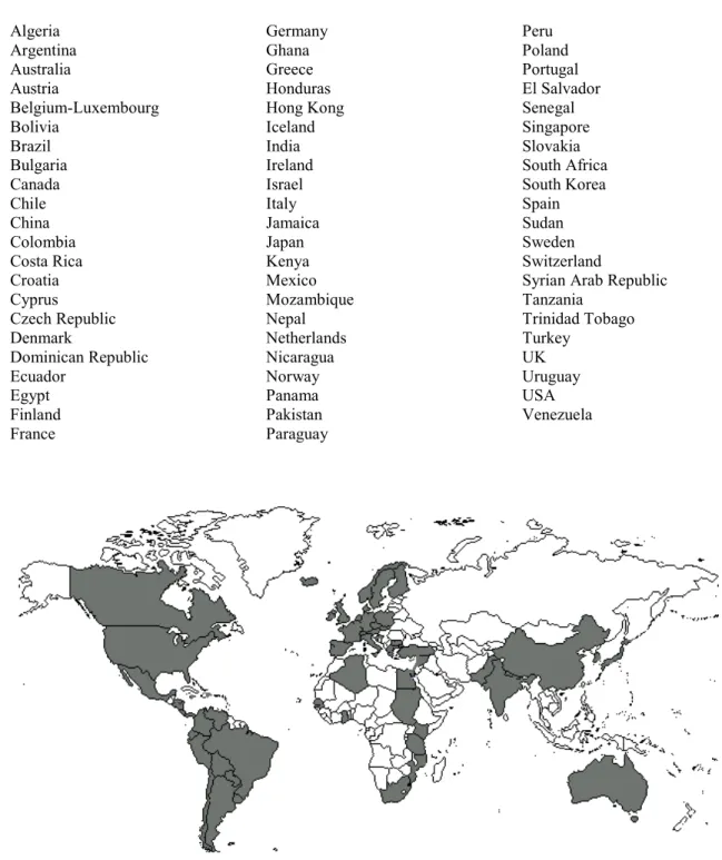
(12) Xj, estimates), where Oj and Xj are the outcome and the explanatory variables for observation j. This ratio shows the probability of obtaining a certain outcome conditional on the estimates. The higher the ratio is, the greater the explanatory power of the model will be. The interpretation of coefficients in an ordered logit model also differs explicitly from other models. In discrete choice logit and probit models, the sign of the coefficients denotes the direction of switch, but its magnitude is difficult to interpret. For example, the positive coefficients corresponding to the characteristics of the individuals in the ordered logit model estimated in this paper increase the probability that a pair of countries will be observed in a higher integration category. However, negative coefficients increase the probability that a pair of countries will be observed in a lower integration category.. 4. Data, hypothesis and variables 4.1. The data The model is estimated with the data of 66 countries from 1999, representing over 75% of world trade (see Table A.1, Appendix A). Data on income are obtained from the World Development Indicators (2001). Distances are the great circle distances between economic centres. Data on capital labour ratios are obtained from the Penn World Tables. Data on bilateral exports are obtained from Statistics Canada (2001), and tariff barriers from the World Bank website. Information about geographical and language dummies is from the CIA (2003). The Economic Freedom Index was obtained from the Heritage Foundation, and the political regime, from the Freedom House. Table A.2 in Appendix A presents a more detailed description of data and sources. Finally, the agreements considered to build the dependent variable are listed in Table A.3 (Appendix A).. 12.

(13) 4.2. Hypothesis and variables According to the underlying theory described above, and in the context of the discrete choice model, our first hypothesis is that a pair of countries will be more likely to form or enhance an RIA when the distance between them is small. We specify the distance variable as in BB. This variable is called “natural” as it is defined as the logarithm of the inverse of distance between trading partners. A second hypothesis is that the probability of RIA formation or enhancement increases as the remoteness of a country or pair of countries from the rest of the world rises. For comparative purposes, we constructed the same remoteness variable used by BB. When a country is relatively far from its trading partners, it tends to trade more bilaterally with its neighbours, thereby increasing the probability of RIA formation. The third hypothesis is that the larger the economic size of the trading countries, the greater the probability of RIA formation or enhancement will be. RGDPij measures the sum of the logs of real GDPs of countries i and j in 19604. The fourth hypothesis is that the more similar the countries’ economic size is, the higher the probability of RIA formation or enhancement will be. DRGDPij is the absolute value of the difference between the logs of real GDPs of countries i and j in 1960. The fifth hypothesis is that the larger the countries’ economic size outside the RIA is, the lower the probability of RIA formation or enhancement will be. However, the size of the rest of the world (ROW) measured by the ROW GDP varies only slightly in a cross-section of countries and has not been included in the regression. BB obtained a non-significant coefficient for this variable. The sixth hypothesis is that the probability that a pair of countries will form or enhance an RIA is higher if there is a larger difference in their relative factor endowments since 4. Data are from 1960 to avoid the problems derived from the endogeneity of income in the estimated equation. The same applies to variables DRGDPij and DKLij.. 13.

(14) traditional comparative advantages will be further exploited. However, if intercontinental transport costs are low, this probability may also decrease at high levels of specialisation. This can be modelled by adding a quadratic term to the estimated equation. We use absolute differences in the capital stock per worker ratio (DKLij) as a proxy for relative factor endowment differences, as in BB5. SQDKLij denotes squared DKLij. The seventh hypothesis is that more democratic countries display a greater likelihood of concluding RIAs than other countries, as stated by Mansfield, Milner and Rosendorff (2002). The eighth hypothesis is that a pair of countries is more likely to form or enhance an RIA than if they have a higher level of economic freedom and if they speak a common language. The ninth hypothesis is that interior countries (landlocked) as well as adjacency countries will have a higher probability of engaging in an RIA, especially with coastal countries. However, when a landlocked country trades with partners located in another continent (unnatural partner), it will have higher transport costs than a coastal country. Finally, the tenth hypothesis is that countries with higher levels of protection (tariffs) will have more incentives to create or enhance an RIA with other countries in order to lower (or eliminate) artificial trade barriers and to facilitate trade. Supplementary economic, geographical and socio-political variables are added to the list of variables used by BB as determinants of RIAs (hypotheses 7-10). Landlocked status and adjacency are added to the list of geographical variables used by BB. The socio-political variables considered are: tariff barriers, sharing a common language, the political regime (this variable takes a value of 1 when the political regime was a 5. Data are for 1965 rather than 1960, since data on capital labour ratios is only available from 1965 onwards in the Penn World Tables data series. Baier and Bergstrand (2004) use data for 1960.. 14.

(15) democracy in 1950)6, and the level of economic freedom. The economic freedom variable takes a value between 1-1.99 for free countries, 2-2.99 for mostly free countries, 3- 3.99 for mostly non-free countries and 4-4.99 for repressed countries. According to the hypotheses above, tariffs, language and democracy are expected to have a positive sign, and economic freedom is expected to have negative coefficients7. Bilateral trade flows were initially added as an economic variable. Trade flows were expected to have a positive sign since more trade between countries indicates a strong relationship and dependence, and a reason to sign an RIA. However, due to the endogeneity problems found for bilateral trade, we chose to exclude this variable from the estimations. Magee (2003) provides one of the first assessments of the hypothesis that two countries are more likely to form a PTA if they are already major trading partners. He estimates a probit and a non-linear two-stage least squares model that considers trade flows to be endogenous in the second specification. Magee’s results show that greater bilateral trade flows significantly increase the likelihood that countries will form a preferential trade agreement in every specification of the model. The first model estimated is a binary probit; the dependent variable takes the value of one when the countries reach an integration agreement, and zero otherwise, and the independent variables are those listed above. The second model estimated is an ordered logit. Five different possible levels of integration between pairs of countries are considered to investigate the determinants of regional integration agreements (RIAs). The variables included are the same, but the interpretation of the estimated coefficients is slightly different.. 6. Data for this variable were only available for the years 1950 and 2000. To avoid the problems derived from the endogeneity of democracy in the estimated equation, we used the data from 1950. 7 Note that according to the definition of these variables, higher values imply lower economic freedom.. 15.

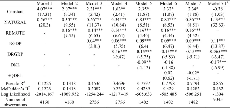
(16) 5. Estimation Results 5.1. Probit estimation The results obtained when a binary probit is estimated are shown in Tables 1 and 2. The results in Table 1 will be comparable to those obtained by BB8, although the sample of countries considered is not exactly the same, the year is 1999 instead of 1996, and the definition of the dependent variable also varies slightly.. Table 1. Probit results for the probability of RIA formation.. The first hypothesis to be tested is that the smaller the distance between the two countries, the more likely their social planners will be to form an RIA, since the closer the two trading partners are, the fewer their trade barriers will be. The probability of establishing an RIA increases with diminishing distances between the trading countries. BB obtain a positive coefficient (1.74) in their equivalent Model 1. We also obtain a positive coefficient (0.56), but it is lower in magnitude. The second hypothesis is tested in Model 2. For a given distance between two countries, the more remote the two continental trading partners are from the rest of the world, the more likely they will be to form an RIA. We calculate this variable according to BB and we obtain a positive coefficient that is similar in magnitude. In Model 3, the third hypothesis is that the larger the trading partners are in economic terms, the greater the probability of an RIA being formed will be. This effect is captured by RGDPij, and it is positive and significant, as expected. However, the coefficient obtained in this paper is lower than that obtained in BB.. 8. Table B.1 in Appendix B.. 16.

(17) In Model 4, the fourth hypothesis is tested. The greater the similarity between the economic size of the two countries, the higher the probability of an RIA being established will be. This effect is captured by DRGDPij. We obtain the expected negative sign and this variable is significant. Finally, the sixth hypothesis is tested in Models 5, 6 and 7. According to BB, the larger the difference between countries’ relative factor endowments, the greater the probability of FTA formation will be, although this may only be true to a limited extent. Variables DKLij and SQDKLij (DKLij squared) measure this effect. When we include these two variables in the same regression, they are not significant. Since the two variables are highly correlated, DKLij and SQDKLij are included in Models 5 and 7 respectively. Both variables are significant, but they do not have the expected signs. The negative sign obtained for DKLij indicates that the larger the difference between countries’ relative factor endowments is, the lower the probability of an RIA will be. This result indicates that the social planners from the two countries tend to form an RIA when they have similar relative factor endowments. Accordingly, higher levels of intra-industry trade will be desirable if RIAs are to be formed, since countries with similar endowments trade similar commodities. This does not support the notion of “natural trading partners” defined by Schiff (1999) as being complementary between partners (one country tends to import what the other exports). A plausible explanation from the demand side may be that because countries with similar endowments have similar tastes and love variety, their governments will be more likely to negotiate higher levels of integration. BB test an additional hypothesis. The higher the absolute difference between the relative factor endowment of the member countries and the relative factor endowment of the ROW, the lower the probability of FTA formation will be, due to potential trade. 17.

(18) diversion. We construct DROWKLij according to BB, although we aggregate the ratio K/L rather than aggregating both variables separately9 since we do not have detached data for capital and labour. We use Equation (9) to calculate DROWKLij.  N   N  { log  ∑ [K k / Lk ] − log[K i Li ] + log  ∑ [K k / Lk ] − log K j L j }  k =1,k ≠ i  k =1, k ≠ j  DROWKLij = 2. [. ]. (9). The coefficient of this variable is close to zero (0.05) and is not significant. Differences in the two sets of results can be explained by the different constructions of the dependent variable: BB consider only full FTAs or customs unions (CUs), whereas our dependent variable includes all PTAs, FTAs, CUs, SMs and MUs notified to GATT/WTO under Article XXIV and under the Enabling Clause (see Table A.3, Appendix A). This variable is broader since it regards integration agreements as a process with different levels of integration; it makes sense to estimate an ordered logit with this construction. BB use the Pseudo R2, calculated according to Equation (7) above, as a measure of explanatory power. However, Heinen (1993) points out that although this index is not affected by changes in sample size, it is affected by the presence of missing observations.10 In this case, a better alternative is to calculate McFadden’s R2 which takes the missing values into account. Table 1 shows both Pseudo R2 and McFadden’s R2. The McFadden statistic considers that there is a different number of observations in the restricted and unrestricted models when there are missing values for some variables.. 9. Baier and Bergstrand (2004) measure DROWKLij as:. DROWKLij=.  N  { log ∑ K k   k =1,k ≠ j .  N   N   ∑ Lk  − log[K i Li ] + log ∑ K k     k =1,k ≠ j   k =1,k ≠i  2. 10.  N   ∑ Lk  − log K j L j }  k =1,k ≠i . BB did not have missing observations. Therefore in the context of their empirical exercise, the pseudo R-squared seems appropriate.. 18. [. ].

(19) In the estimated Models 3-7, McFadden’s R2 is preferred to Pseudo R2 since there are zero values in some of the explanatory variables. In order to have a clear representation of the relative importance of the additional geographical and socio-political variables, a probit model extended with those variables was also estimated. The main results are reported in Table 2.. Table 2. Probit results for the probability of RIA formation: Extended model.. In the first column of Table 2 (Model 5) the same results reported in Table 1 are also included for comparative purposes. Model 8 to Model 12 in columns 3 to 7 of Table 2 are estimated for different sets of variables grouped as geographical (Models 8 and 9), economic and geographical (Model 10), socio-political variables (Model 11) and all the variables (Model 12). This sequential analysis enables us to find out the most important factors in promoting RIAs using the simple probit model. Models 8 and 9 in Table 2 show the results of the geographical variables. All geographical variables are significant at 1%, and natural, remoteness and adjacency have a positive signed coefficient, while the landlocked variable coefficient is negative. In Model 9, the interaction variable (landlocked*remoteness) is added to investigate the reasons why the landlocked variable is negatively signed. The estimated coefficient for the interaction term is positive, indicating that the probability of joining an RIA increases for more remote continental trading partners when one of them is landlocked. Geographical variables alone explain 16% of the variability of the dependent variable. Model 10 reports the results of adding economic and geographical variables. In this extended model, the dummies landlocked and adjacency are not statistically significant and the former shows a positive sign. Model 11, in column six of Table 2, shows that all. 19.

(20) the socio-political variables are significant: democracy, the level of economic freedom, the common language and higher tariffs promote RIAs formation. However, in terms of goodness of fit, Pseudo R2 is very low (0.05). Finally, Model 12 reports the results with economic, geographical and socio-political variables. In this model an additional interaction variable has been included (natural*language) since the effect of the common language dummy is only positive and significant when it is interacted with the “natural” variable. The adjacency variable is not significant and the language dummy initially showed an unexpected negative sign that reverses when the variable is interacted with the “natural” variable.. 5.2. Ordered logit estimation We estimate an ordered logit model consisting of a system of 5 equations with common coefficients for all the explanatory variables and with different constant terms. This is known as the proportional odds model. In the first column of Table 3 (Model 13), an ordered logit is estimated with the same variables included in Model 5 (probit estimation). Model 14 to Model 16 in columns 3 to 5 of Table 3 are estimated for different sets of variables grouped as economic, geographical, socio-political variables, and Model 17 includes all the variables. This sequential analysis enables us to find out the most important factors in promoting RIAs.. Table 3. Ordered logit results for the probability of RIA formation or enhancement.. Model 13 shows that the results are similar in both probit and ordered logit models, although the logit ordered coefficients are higher in magnitude. In general terms, we can state that the probability of reaching a higher level of integration is higher than the. 20.

(21) probability of signing any type of RIA when no previous agreement exists between the trading countries. However, as stated above, there is no consensus on the interpretation of the magnitude of the coefficients estimated in discrete choice models. Models 14 and 15 in Table 3 show the results of the geographical variables. All geographical variables are significant at 1%, and natural, remoteness and adjacency have a positive signed coefficient, while the landlocked variable coefficient is negative. In Model 15 the interaction variable (landlocked*remoteness) is added to consider the ambiguous sign expected for the landlocked variable. The estimated coefficient shows a positive sign, indicating that the probability of reaching a higher level of integration increases for more remote continental trading partners when one of them is landlocked. Model 16, in column six of Table 3, shows that all the socio-political variables are significant: democracy, the level of economic freedom and the common language promote RIA enhancement. However, in terms of goodness-of-fit, Pseudo R2 is very low (0.04). The coefficient on tariffs is positive, thus showing that a higher level of protection increases the probability that a country pair will be observed in a higher category. Finally, Model 17 includes economic, geographical and socio-political variables. Some interaction terms were also added to allow for the possibility that the effect of some variables, namely remoteness and language, could be different for natural and unnatural patterns. In this model, remoteness presents a negative sign, indicating that remote countries have a lower probability of reaching higher levels of integration, while the variables adjacency, language and tariffs are not statistically significant. The Akaike Info Criterion (AIC) shows that the best specification is that estimated in Model 17, where all the variables are considered. For the specification where only geographical variables are considered, the AIC is lower (1.542) than that obtained in. 21.

(22) regressions including only socio-political factors (1.681). This appears to indicate that geographical variables are important determinants of RIA formation. As stated above, the interpretation of the coefficients in an ordered logit does not inform of the magnitude of switch since we can only state that positive coefficients increase the likelihood that the country pairs will be observed in a higher category, and negative coefficients increase the likelihood that the country pairs will be observed in a lower category. A preferable interpretation of the ordered logit coefficients is in terms of the odd ratios. The exponentiated coefficients in the logit model, shown in Table 4, can be interpreted as odds ratios for a 1-unit change in the corresponding variable. The emphasis is on the ratio “Exp(β)”, which is the odds conditional on x+1 divided by the odds conditional on x. For example, 1.19 means that the odds of being in a higher integration level increase by 1.19 if RGDP increases by 1. The interpretation can also be made in terms of percentages: the exp(1.49) obtained in the “natural” variable in Model 13 means that the odds increase by 346% {[exp(1.49)-1]*100} if the variable increases by 1, therefore the odds of being part of the monetary union versus lower integration levels is 346% higher for a one-unit increase in the “natural” variable. Table 4 shows that, in Model 13, the most important determinant of an RIA is the “natural” variable, followed by remoteness (1.37), real GDP (1.19), real GDP differences (0.84) and K/L differences (0.77). We also calculate semi-standardised ordered logit coefficients that control for the metrics of the independent variables to see whether any change occurs in the ordering of effects. The option of standardised coefficients to measure the relative strength of the effects of the independent variables is more appropriate in the current empirical application since some independent variables are measured in different units. Table 4 shows that when standardised coefficients are considered (e^bStdX), the ordering of the. 22.

(23) effects changes only slightly. In Model 13, the natural variable’s standardised coefficient is 3.89, and it is 1.76 for remoteness, 1.65 for RGDP, 0.75 for K/L differences, and 0.74 for real GDP differences. For one standard deviation increase in “natural”, the odds are 3.89 times greater (an increase of 289%) of countries being in a higher integration category when all the other variables are held constant. In Model 17, where socio-political variables are added, the natural variable is still the most important followed by real GDP and democracy.. Table 4. Odds ratios for the ordered logit.. In order to evaluate the probability that the dependent variable will have a particular value, we use cut-offs terms. From Equation (1), the threshold parameters for Model 13 are given by: Yi = 0 if Y*i ≤ -3.41 Yi = 1 if –3.41 ≤ Y*i ≤ -2.71 Yi = 2 if –2.71 ≤ Y*i ≤ -1.8 Yi = 3 if –1.8 ≤ Y*i ≤ -1.58 Yi = 4 if –1.58 ≤ Y*i ≤ 0.38 Yi = 5 if Y*i ≥ 0.38 For example, when the trading partners are Argentina and Paraguay, we can calculate the probability associated with this pair of countries by computing Zi with the obtained coefficients in Model 13 and the corresponding data:. Z i = β 1 ⋅ RGDPij + β 2 ⋅ DRGDPij + β 3 ⋅ DKLij + β 4 ⋅ REMOTE + β 5 ⋅ NATURAL = = (0.18 ⋅ 46.7) + (−0.17 ⋅ 4.22) + (−0.26 ⋅ 3.3) + (1.49 ⋅ (−6.94)) + (0.31 ⋅ 3.98) = − 2.28 1 Pr(Y = 0) = Pr ( Z i ≤ 0 ) = = 0.2442 1 + exp(− 2.28 − ( −3.41) ). 23.

(24) 1 1 − = 0.1499 1 + exp(− 2.28 − (−2.71) ) 1 + exp(− 2.28 − (3.41) ) 1 1 Pr(Y = 2) = Pr ( Z i ≤ δ 2 ) − Pr ( Z i ≤ δ 1 ) = − = 0.2236 1 + exp(− 2.28 − (−1.8) ) 1 + exp(− 2.28 − (−2.71) ) 1 1 Pr(Y = 3) = Pr ( Z i ≤ δ 3 ) − Pr ( Z i ≤ δ 2 ) == − = 0.0505 1 + exp(− 2.28 − (−1.58) ) 1 + exp(− 2.28 − (−1.8) ) 1 1 Pr(Y = 4) = Pr ( Z i ≤ δ 4 ) − Pr ( Z i ≤ δ 3 ) = − = 0.2664 1 + exp(− 2.28 − (0.38) ) 1 + exp(− 2.28 − (−1.58) ) Pr(Y = 1) = Pr ( Z i ≤ δ 1 ) − Pr ( Z i ≤ 0 ) =. Pr(Y = 5) = Pr (δ 5 ≤ Z i ) = 1 −. 1 = 0.0654 1 + exp (− 2.28 − ( 0.38 ) ). Hence for Argentina and Paraguay, the most likely outcome is that they will form a single market. In fact, they have been members of Mercosur since 1995. Our second example is Spain and France, a pair of trading partners that are members of the European Union. Our results indicate that the highest probability is that of the establishment of a single market. In 1999 these countries were already in the third phase of the European Monetary Union (EMU), since they fulfilled the convergence criteria established in the Treaty of Maastricht. However, our results most probably show that they were only in the EMU starting phase.. Z i = β 1 ⋅ RGDPij + β 2 ⋅ DRGDPij + β 3 ⋅ DKLij + β 4 ⋅ REMOTE + β 5 ⋅ NATURAL = = (0.18 ⋅ 52.6) + (−0.17 ⋅ 1.24) + (−0.26 ⋅ 0.732) + (1.49 ⋅ (−6.96)) + (0.31 ⋅ 3.75) = − 0.14 1 = 0.0366 1 + exp(− 0.14 − ( −3.41) ) 1 1 = 1) = Pr ( Z i ≤ δ 1 ) − Pr ( Z i ≤ 0 ) = − = 0.0345 1 + exp(− 0.14 − (−2.71) ) 1 + exp(− 0.14 − (−3.41) ) 1 1 = 2) = Pr ( Z i ≤ δ 2 ) − Pr ( Z i ≤ δ 1 ) = − = 0.0887 1 + exp(− 0.14 − (−1.8) ) 1 + exp(− 0.14 − (−2.71) ) 1 1 = 3) = Pr ( Z i ≤ δ 3 ) − Pr ( Z i ≤ δ 2 ) == − = 0.0318 1 + exp(− 0.14 − (−1.58) ) 1 + exp(− 0.14 − (−1.8) ) 1 1 = 4) = Pr (Z i ≤ δ 4 ) − Pr (Z i ≤ δ 3 ) = − = 0.4356 1 + exp(− 0.14 − (0.38) ) 1 + exp(− 0.14 − ( −1.58) ) 1 = 5) = Pr (δ 5 ≤ Z i ) = 1 − = 0.3728 1 + exp (− 0.14 − (0.38) ). Pr(Y = 0) = Pr ( Z i ≤ 0 ) =. Pr(Y Pr(Y Pr(Y Pr(Y P (Y. 24.

(25) When the socio-political variables are also considered (Model 17), then the threshold parameters are given by: Yi = 0 if Y*i ≤ -14.82 Yi = 1 if -14.82 ≤ Y*i ≤ -14.01 Yi = 2 if -14.01 ≤ Y*i ≤ -13.23 Yi = 3 if -13.23 ≤ Y*i ≤ -12.91 Yi = 4 if -12.91 ≤ Y*i ≤ -10.41 Yi = 5 if Y*i ≥ -10.41 Therefore, for the second example (Spain and France), our results indicate that the highest probability is that of the establishment of a monetary union. Z i = β 1 ⋅ RGDPij + β 2 ⋅ DRGDPij + β 3 ⋅ DKLij + β 4 ⋅ REMOTE + β 5 ⋅ NATURAL + β 6 ⋅ ADJij + β 7 ⋅ LANDij + + β 8 ⋅ LANDij ⋅ REMOTE + β 9 ⋅ NATURAL ⋅ REMOTE + β 10 ⋅ LANGij + β 11 ⋅ DEM 50ij + β 12 ⋅ FREEDOMij + + β 13 ⋅ TRADE _ BARRIERS + β 14 ⋅ NATURAL ⋅ LANGij = - 11.11. Pr(Y = 0) = Pr (Z i ≤ 0 ) =. 1 = 0.024 1 + exp(− 11.11 − (−14.82) ). Pr(Y = 1) = Pr (Z i ≤ δ 1 ) − Pr (Z i ≤ 0 ) =. 1 1 − = 0.028 1 + exp(− 11.11 − (−14.01) ) 1 + exp(− 11.11 − ( −14.82) ). Pr(Y = 2) = Pr (Z i ≤ δ 2 ) − Pr (Z i ≤ δ 1 ) =. 1 1 − = 0.055 1 + exp(− 11.11 − (−13.23) ) 1 + exp(− 11.11 − (−14.01) ). Pr(Y = 3) = Pr (Z i ≤ δ 3 ) − Pr (Z i ≤ δ 2 ) == Pr(Y = 4) = Pr (Z i ≤ δ 4 ) − Pr (Z i ≤ δ 3 ) = Pr(Y = 5) = Pr (δ 5 ≤ Z i ) = 1 −. 1 1 − = 0.034 1 + exp(− 11.11 − (−12.91) ) 1 + exp(− 11.11 − (−13.23) ). 1 1 − = 0.526 1 + exp(− 11.11 − (−10.41) ) 1 + exp(− 11.11 − (−12.91) ). 1 = 0.667 1 + exp (− 11 .11 − ( −10 .41) ). The calculation of the predicted probabilities for all the trading partners11 shows that 69% of the agreements and 84% of the non-agreements were correctly predicted by the ordered logit model. Of all cases, 17% had excessive bilateralism12, i.e., when the. 11 12. Model 13. “Excessive” and “insufficient” bilateralism are terms used by BB.. 25.

(26) predicted level of integration was lower than the real level, and we found that bilateralism was insufficient for 6.5% of the trading partners.. 5.3. Marginal effects As BB point out, “one complication arises in estimating the partial effects on the response probabilities for the particular vector of RHS variables, x, in our model by using mean values for the levels. One of the RHS variables, REMOTE, is the product of a continuous variable and a binary variable (…) the mean value of this variable is economically meaningless”.13 As we also use REMOTE, we estimate separately the marginal effects on the response probabilities with the mean value of REMOTE when the trading partners are in the same continent, and when REMOTE takes the value of zero (the trading partners are not in the same continent, they are unnatural partners). Marginal effects are calculated for Model 12 (probit) and Model 17 (ordered logit).14 Our results for the probit estimation are shown in Table 5 and for the ordered logit estimation in Table 6. Our results in Table 5 can be compared with those obtained by BB, shown in Appendix B (Table B.2), although we include two additional sociopolitical variables (economic freedom and trade barriers) that were not considered by BB.. Table 5. Response probabilities for natural and unnatural trading partners in Model 12 (evaluated at the mean level of remote and at remote = 0).. Table 5 shows that the response probability of an RIA being created is much lower for unnatural partners (5.8%) than for natural partners (88.5%). Moreover, results show that 13. Baier and Bergstrand (2004), page 55. Dummy variables are not included since the mean values of these variables do not have an economic interpretation. 14. 26.

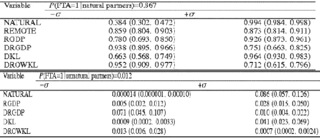
(27) a unitary increase in proximity (natural variable) increases this probability by 7.3% for two natural partners and 11.8% for unnatural partners. An increase in remoteness from the ROW of two natural partners lessens the response probability in natural partners. Although this is an unexpected result, Table 6 shows that the sign of this marginal effect changes for different levels of integration when the model estimated is an ordered logit rather than a binary probit model. This sign is only positive for the first two integration stages (PTA and FTA). When two countries are in the same continent and they are relatively far away from the other countries in this continent, then the probability that they will reach a customs union decreases with the level of remoteness. The results show that economic variables have a lower effect than geographical and socio-political factors on response probabilities, although differences in income also play an important role in RIA formation. The response probability for natural partners is similar to that obtained by BB, who find 86.7% probability of an FTA being established between natural partners. However, they only obtain a probability of 1.2% for unnatural partners. We obtain a higher probability for unnatural partners because we also considered preferential trade agreements in the construction of the dependent variable. To compare the effect of the RHS variables across different levels of integration, in Table 6 we estimate the marginal effects for all the integration levels for both natural and unnatural partners.. Table 6. Response probabilities for natural and unnatural trading partners in Model 17 (evaluated at the mean level of remote and at remote = 0).. 27.

(28) Table 6 shows different probabilities depending on the level of integration. For each level of integration, the probabilities are shown for natural and for unnatural partners. However, for the three last categories (customs union, single market and monetary union) the probabilities can only be calculated for natural partners since these integration levels are only reached by countries in the same continent. These probabilities depend mainly on geographical, socio-political and economic variables, and their marginal effects differ across integration levels. On the one hand, the results obtained for natural partners (countries in the same continent) indicate that when remoteness increases by 1%, the probability of a PTA or an FTA being established increases by 337% and 159%, respectively. However, the probability of a customs union or a higher integration agreement being established decreases with remoteness. This variable, together with socio-political factors, is the most influential factor on the probability of an RIA being formed or enhanced between natural partners. Higher GDP differences increase the probability of PTA or FTA formation for natural partners, although the sign of the marginal effect for higher levels of integration is reversed, thus indicating that similarity of income, as expected, increases the probability that higher levels of integration (customs union, single market and monetary union) will be reached. The integration theory predicts that the costs of integration are lower when countries have similar levels of income and, consequently, a high level of intra-industry trade. For unnatural partners however (countries in a different continent), the inverse of distance is the most important factor in PTA or FTA formation, and higher differences in income and in factor endowments lower the probability of a PTA or an FTA being established.. 28.

(29) Finally, the results show the most likely outcomes are that natural partners will establish a single market and unnatural partners will not reach any agreement. When we order the probabilities for the various types of integration agreements from the highest probability to the lowest probability for natural partners, we obtain: Pr(SM or 4) = 0.38 Pr(FTA or 2) = 0.19 Pr(PTA or 1) = 0.17 Pr(CU or 3) = 0.12 Pr(MU or 5) = 0.03 These findings can seem surprising since the (conventionally assumed) second most integrated type of agreement, a single market, is the most likely type of RIA. An explanation is that the results obtained are likely to be dominated by the European Common Market.. 5.4. Sensitivity Analysis We performed several robustness tests to validate our results. Firstly, the ordered logit model is based on the assumption of parallel slopes but this may be unrealistic, for example, if geographical variables are less relevant for higher integration levels. Therefore, the Brant test of the parallel regression assumption is used to validate the methodology used. The Brant (1990) test assesses whether or not the coefficients are the same for each category of the dependent variable. This produces Wald Tests for the null hypothesis that the coefficients in each independent variable are constant across categories of the dependent variable. Significant test statistics provide evidence that this assumption has been violated for most of the variables. With the exception of the capital-labour ratio, we cannot accept the equality of slopes for the different levels of integration (Table A.4). These results indicate that we should estimate a generalised. 29.

(30) logit model, and they suggest what variables may be used in determining the thresholds. We therefore estimated a generalised ordered logit for all the regressions presented in Table 3. In some cases, the model did not converge, especially when the variables with missing data (K-L differences) were included. The results15 indicate that the geographical variables are significant and show the expected signs for the lower levels of integration (PTA, FTA), whereas these variables lose significance and decrease in magnitude for the higher levels. In contrast, the economic and political variables gain importance in the higher levels of integration. Secondly, we re-estimated the probit and ordered logit model with an alternative data set taken from Magee (2003), which are available for replications on his web site. His dependent variable takes the value of one if the country pair has a PTA in 1998, and takes zero otherwise. We use the same dependent variable in the probit estimation, but Magee (2003) considers fewer agreements since he ignores the General System of Trade Preferences (GSTP), the Protocol related to Trade Negotiations among developing countries (PTN) and the African Common Market. Additionally, the variable remoteness is not included as an explanatory variable in Magee (2003). We estimate a binary probit for 172 countries in 1998 and our results confirm the sign and significance of the estimated coefficients for the income variables, the relative factor endowment differences and the natural variable (Model 7.1 in Table 1). Contrary to BB, the K-L differences variable is negative and significant, thus validating our evidence. Similar results are obtained when an ordered logit is estimated. Thirdly, we also estimated the probit model with the inclusion of bilateral trade as an explanatory variable and using instrumental variables to correct endogeneity problems. Infrastructure variables were used as instruments for trade. The results indicate that. 15. Results are available upon request from the authors.. 30.

(31) trade is significant and has a positive sign when it is added to the list of explanatory variables in the probit model, confirming the evidence presented by Magee (2003) with different data and different model specifications. However, as stated above further research is needed to improve the model specification. Fourthly, the observations are twice the number of country pairs. However, our dependent variable is symmetric and only trade and tariffs are asymmetric ( X ij ≠ X ji ). Therefore, we have re-estimated the model with only half the observations to check whether this would have affected the results. By taking 2145 ((66*65)/2) country pairs, the results remained unchanged.16 Fifthly, an additional robustness test has been performed. We checked whether the results were affected by the exclusion of an important economic bloc, such as the EU. The results excluding the EU countries also remained unchanged.17 Finally, the ordered nature of the dependent variable and the endogeneity of trade flows should ideally be considered simultaneously, although this is beyond the scope of this research.. 6. The dynamics of the European Union integration process The EU is the best real example of a successful integration process. However, the fact that the analysis in the previous sections focuses on data for 1999 covers neither the entrance of 10 countries into the EU in 2004 nor the adoption of the Euro by Greece.18 In order to tackle the above-mentioned issues, the proposed model has been estimated for an additional sample, including data for the EU-27 from 1999 to 2007. A dynamic analysis would also be possible by adding the time dimension to the data.. 16. The results of taking into account the “repetition bias” in the 66-country sample are available upon request from the authors. 17 These results are available upon request from the authors. 18 A referee kindly suggested the inclusion of this section in the paper.. 31.

(32) In relation to the socio-political factors, democracy in 1950 was used in Section 5. Nonetheless, this variable may have very little to do with the probability of a country pair forming or enhancing an RIA during the period 1999-2007 in Europe. Although Spain and Portugal were dictatorships in 1950, both restored democracy in the mid1970s, and joined the European Community (EC) in 1986. Greece also restored democracy in the mid-1970s and joined the EC in 1981. Hence, these three countries were democracies at the time they joined the EC. The same applies to the former socialist countries that joined the EU in 2004 and 2007. Therefore, unlike the analysis performed in Section 5, we take into account the political regime at the time of entry into the EC and not the situation in 1950. Instead of a dummy variable for democracy, the variable policy is used. 19 Political rights and civil liberties at the time of entry into the EC have also been added to the list of political variables. They are measured on a one-to-seven scale, with one representing the highest degree of freedom and seven the lowest.20 Table 7 shows the results obtained for the EU-27 sample. In the first column of Table 7 (Model 18), an ordered logit is estimated with the same variables included in Model 13 (Table 3).21 Model 19 to Model 21, in columns 2 to 4 of Table 7 report the results for models with different sets of variables grouped as geographical and socio-political variables. Finally, Model 22 includes all the variables, as does Table 3.. 19. Annual data for democracy are obtained from the Polity IV dataset (http://www.systemicpeace.org/inscr/p4v2007.xls). The variable POLITY2, which varies from -10 (strong dictatorship) to 10 (full democracy), is used in Section 6. 20 Annual data on political rights and civil liberties are obtained from The Freedom House (2009): http://www.freedomhouse.org/uploads/fiw09/CompHistData/FIW_AllScores_Countries.xls 21 DKL is not included in the analysis for the European integration process since DKL was not significant in the deepest integration levels (see Table 6). Remoteness is also calculated for the European country sample as was done in Baier and Bergstrand (2004), however, this variable is not included in the regressions since is not considered as comparable to the one constructed for the 66-country sample which includes unnatural partners.. 32.

(33) Table 7. Ordered logit results for the probability of RIA formation or enhancement. The European integration process.. Model 18 shows that the sign of the coefficients for the EU-27 sample is similar to the obtained for the 66-country sample (Model 13), although the coefficients are lower in magnitude. Model 19 shows the results of the geographical variables. All the geographical variables are significant at 1% and have the expected sign. Natural and adjacency have a positive-signed coefficient, while the landlocked variable coefficient is negative. Model 20 shows that all the socio-political variables are significant: democracy, the level of economic freedom (property rights and civil liberties) and the common language promote RIA enhancement. Model 21 includes an additional variable (trade barriers), measuring the bilateral weighted tariffs between trading partners before accessing the EU-27. Unlike the results found in Table 3, the coefficient of this variable is negative, showing that a higher level of protection lowers the probability of a country pair being observed in a higher category in the European Union integration process. Model 22 includes economic, geographical and socio-political variables, excluding democracy which correlates with the GDP. In this model, all the variables present the expected sign and are statistically significant. Model 23 includes a lagged dependent variable that indicates the previous integration level. This variable takes into account the fact that the probability of reaching an integration level depends on the point of departure (i.e., countries that do not have a previous agreement do not usually go straight into a monetary union). The results show that the probability of reaching a deeper integration level is higher if the countries already participate in an RIA. Finally as in BB (2004), the previous specifications assumed that RIAij is independent across observations. Since this assumption is not very realistic and could influence the estimation results, we followed the method proposed by Pesaran (2006) to account for. 33.

(34) interdependencies. This method consists in approximating the linear combinations of the unobserved factors by cross-section averages of the explained and explanatory variables and then running standard panel regressions augmented by the cross-section averages. This approach also yields consistent estimates when the regressors correlate with the factors. The results are presented in Model 24 and indicate that interdependencies matter (the added variables are statistically significant) but do not alter the sign of the estimated coefficients of the variables included in Model 22. As in Section 5, we evaluate the probability of the dependent variable having a particular value. Then we take the case of Spain and France22 in which our results for both the 66-country and EU-27 samples indicate that the highest probability is that of the establishment of a monetary union when socio-political variables were considered (Model 17 and Model 22, respectively). Z i = β1 ⋅ RGDPij + β 2 ⋅ DRGDPij + β 3 ⋅ NATURAL + β 4 ⋅ ADJij + β 5 ⋅ LANDij + + β 6 ⋅ LANGij + β 7 ⋅ POLITICAL RIGHTS + β 8 ⋅ CIVIL LIBERTIES = - 2.03. 1 = 0.019 1 + exp(- 2.03 − ( −5.93) ) 1 1 = 2) = Pr (Z i ≤ δ 2 ) − Pr (Z i ≤ δ1 ) = − = 0.412 1 + exp(− 2.03 − ( −2.31) ) 1 + exp(− 2.03 − ( −5.93) ) 1 1 = 3) = Pr (Z i ≤ δ 3 ) − Pr (Z i ≤ δ 2 ) == − = 0.077 1 + exp(− 2.03 − ( −2.00) ) 1 + exp(− 2.03 − ( −2.31) ) 1 1 = 4) = Pr (Z i ≤ δ 4 ) − Pr (Z i ≤ δ 3 ) = − = 0.399 1 + exp(− 2.03 − (0.25) ) 1 + exp(− 2.03 − ( −2.00) ) 1 = 5) = Pr (δ 5 ≤ Z i ) = 1 − = 0.907 1 + exp (− 2.03 − ( 0.25) ). Pr(Y = 0) = Pr (Z i ≤ 0 ) =. Pr(Y Pr(Y Pr(Y Pr( Y. The results indicate that the probability associated with level five is the highest, which is consistent with the fact that France and Spain were members of the European Monetary Union.. 22. For the EU-27 country sample the probabilities are calculated in the year 1999 to be compared to those obtained in Section 5 with the 66-country sample.. 34.

(35) 7. Conclusions In this paper, discrete choice modelling is used to study the determinants of regional trade agreements. A binary probit model and an ordered logit model are estimated, in which geographical, economic and socio-political variables are considered as explanatory variables for RIA formation. Five different integration levels are specified for the dependent variable in the ordered logit estimation. The results from the probit and ordered logit estimations show that the probability of reaching a higher level of integration increases with income level, economic freedom, cultural affinities and remoteness, whereas it decreases with distance, protection levels, income differences and factor endowment differences. Additionally, although economic and geographical variables seem to be the most important determinants of RIA formation, the socio-political factors considered are all statistically significant and their relative importance in explaining RIAs enhancement increases for higher integration levels and for natural partners. The marginal effects, calculated for natural and unnatural trading partners, show that countries in the same continent (natural partners) will most probably establish a single market, whereas countries in different continents (unnatural partners) are most likely to not sign any agreement. This result is new in the RIA literature and should be validated by extending the sample to include more years and countries. The marginal effects also show that some variables, such as remoteness and differences in real GDP, have a positive influence on the formation of an RIA, but only for countries in the same continent and in the early stages of the integration process (PTA, FTA). However, when the categories considered are higher integration levels, the effect of these two variables is reversed. The marginal effect of economic freedom is not statistically significant for. 35.

(36) unnatural partners in the early stages of the integration process (PTA, FTA). However, it shows that a higher level of economic freedom has a positive influence on the enhancement of a RIA from a customs union to a single market and from a single market to a monetary union. The estimation of a trade equation, that considers the formation of RIAs as an endogenously determined explanatory variable, remains an issue for further research.. Acknowledgments We would like to thank Jeffrey Bergstrand for his helpful comments, and also participants in the European Trade Study Group conference held in Dublin and in the Atlantic Economic Conference held in New York. Financial support from the Spanish Ministry of Public Works, Generalitat Valenciana (Regional Valencian Government), and the Spanish Ministry of Education is gratefully acknowledged (P21/08, ACOMP07/102 and SEJ 2007-67548).. References Amemiya, T. (1975): Qualitative Response Models. Ann. Econ. Social Measurement 4, 363-372. Baier, S.L. and Bergstrand, J.H. (2004): Economic Determinants of Free Trade Agreements. Journal of International Economics 64 (1), 29-63. Baier, S.L. and Bergstrand, J.H (2005): Do free trade agreements actually increase members’ international trade?, Working Paper 2005-03, Federal Reserve Bank of Atlanta. Ben-Akiva, M., and Lerman, S. (1985): Discrete Choice Analysis. MIT Press, Cambridge, Massachusetts. Brant, R. (1990): Assessing Proportionality in the Proportional Odds Model for Ordinal Logistic Regression. Biometrics 46, 1171-1178.. 36.

(37) Campbell, B. (2005): The Case Against Continental Deep Integration. Paper presented to the Centre for Trade Policy and Law conference Options for Canada-US Economic Relations in the 21st Century, November 4, 2005. Central. Intelligence. Agency. –CIA–. (2003):. The. World. Factbook.. From. http://www.odci.gov/cia/publications/factbook Endoh, M. (2006): “Quality of Governance and the Formation of Preferential Trade Agreements”, Review of International Economics 14 (5), 758-772. Frankel, J.A., Stein, E. and Wei, S.-J. (1995): Trading Blocs and the Americas: the natural, the unnatural, and the super-natural. Journal of Development Economics 47 (1), 61–95. Frankel, J.A., Stein, E. and Wei, S.-J. (1996): Regional trading arrangements: natural or supernatural. American Economic Review 86 (2), 52–56. Frankel, J.A., Stein, E. and Wei, S.-J. (1998): Continental trading blocs: are they natural or supernatural. In: Frankel, J.A., Editor, , 1998. The Regionalization of the World Economy, University of Chicago Press, Chicago, 91–113. Great circle distances (2003): From http://www.wcrl.ars.usda.gov/cec/java/lat-long.htm Heinen, T. (1993): Discrete Latent Variable Models. Tilburg University Press. The Netherlands. Koppelman, F.S. and Wen, C. (1998): Alternative nested logit models: Structure, properties and estimation. Transportation Research 32 (3), 289-298. Magee, C. (2003): Endogenous preferential trade agreements: An empirical analysis. Contributions to Economic Analysis & Policy 2 (1), 1-17. Mansfield, E. D., Milner, H. V. and Rosendorff, B. P. (2002): Why Democracies Cooperate More: Electoral Control and International Trade Agreements, International Organization 56, 477–513.. 37.

(38) McFadden, D. and Train, K. (2000): Mixed MNL models for discrete response. Journal of Applied Econometrics 15 (5), 447-470. McKinnon, R. (1979): Money in International Exchange: The Convertible Currency System. Oxford. Oxford University Press. Miles, M. A., Feulner Jr., E. J., O’Grady M. A. and Eiras A. I (2004): Index of Economic Freedom. The Heritage Foundation. Penn World Tables (2005): From http://datacentre.chass.utoronto.ca/pwt56/ Schiff, M. (1999), “Will the Real “Natural Trading Partner” Please Stand Up?” World Bank, Development Research Department Working Paper. Statistics Canada (2001): World Trade Analyzer. The International Trade Division of Statistics of Canada. The Freedom House (2005): Democracy’s Century. A Survey of Global Political Change in the 20th Century. From http://www.freedomhouse.org/ Vicard, V. (2006): "Trade, Conflicts, and Political Integration: the Regional Interplays," CESifo Working Paper Series CESifo Working Paper No., CESifo GmbH. Viner, J., (1950): The Customs Union Issue, Carnegie Endowment for International Peace, New York. World Bank (2001): World Development Indicators, Washington. World Bank (2005): From http://www.worldbank.org/ World Trade Organization (1995): Regionalism and the World Trading System. Geneva. World Trade Organization (2005): From http://www.wto.org/ Wu, J. P.(2004): Measuring and explaining levels of regional economic integration. Working Paper B12/2004. Centre for European Integration Studies. From http://www.zei.de/ Wyplosz, C. (2006): Deep Economic Integration: Is Europe a Blueprint?, Asian. 38.

(39) Economic Policy Review 1, 259-279. Table 1. Probit results for the probability of RIA formation.. REMOTE. -. RGDP. -. -. DRGDP. -. -. -. DKL. -. -. -. -. SQDKL. -. -. -. -. -. Pseudo R2 McFadden’s R2 Log Likelihood Number of observations. 0.1226 0.1226 -2014.167. 0.1418 0.1418 -1969.952. 0.4536 0.2087 -1254.244. 0.4696 0.2319 -1217.419. 0.7797 0.4289 -505.633. Model 6 2.32* (1.87) 0.85*** (8.53) 0.16*** (4.44) 0.09*** (6.47) -0.15*** (-5.83) -0.16 (-1.38) 0.02 (0.62) 0.7798 0.429 -505.485. 4160. 4160. 2756. 2756. 1482. 1482. Constant NATURAL. Model 1 4.07*** (17.31) 0.56*** (20.3). Model 2 2.07*** (6.34) 0.35*** (9.55) 0.16*** (9.35). Model 3 2.31*** (3.42) 0.56*** (11.37) 0.14*** (6.65) 0.04*** (3.81). Model 4 1.63** (2.41) 0.54*** (10.64) 0.14*** (6.64) 0.06*** (5.75) -0.16*** (-9.47). Model 5 2.35* (1.88) 0.85*** (8.51) 0.16*** (4.40) 0.09*** (6.4) -0.15*** (-5.75) -0.09** (-2.12). Model 7 2.34* (1.88) 0.86*** (8.51) 0.16*** (4.32) 0.09*** (6.44) -0.15*** (-5.71) -0.02* (-1.71) 0.7794 0.4282 -506.251 1482. Model 7.1a -0.78 (-1.03) 1.19*** (32.63) 0.11*** (13.87) -0.065*** (-3.47) -0.17*** (-6.99) -. Notes: ***, **, * indicate significance at 1%, 5% and 10%, respectively. Z-statistics are in brackets. The dependent variable is a binary discrete variable that takes the value of 1 when trading partners were integrated into a PTA, FTA, CU, SM and MU in 1999, and 0 otherwise. The Huber/White/sandwich estimator of variance is used instead of the traditional calculation, therefore the estimation uses heteroscedasticity-consistent standard errors. a Model 7.1 was estimated with an alternative data set for a cross-section of 172 countries in 1998 from Magee (2003).. 39. 0.865 0.462 -1304 9045.

(40) Table 2. Probit results for the probability of RIA formation: Extended model.. ADJACENCY. Model 5 0.09*** (6.40) -0.15*** (-5.75) -0.09** (-2.12) 0.85*** (8.51) 0.16*** (4.40) -. LANDLOCKED. -. LANDLOCKED*REMOTE. -. 0.31*** (7.99) 0.16*** (9.24) 0.70*** (5.03) -0.32*** (-5.43) -. LANGUAGE. -. -. 0.30*** (7.65) 0.14*** (7.97) 0.69*** (4.98) -0.49*** (-5.75) 0.10*** (3.07) -. DEMOCRACY. -. -. -. RGDP DRGDP DKL NATURAL REMOTE. Model 8 -. Model 9 -. -. -. -. -. Model 10 0.10*** (4.82) -0.14*** (-5.64) -0.15** (-2.96) 0.86*** (8.76) 0.12*** (3.13) 0.03 (0.12) 0.04 (0.25) 0.17** (2.71) -. Model 11 0.36*** (5.47) 0.87*** (10.96) -0.29** (-2.47) 0.25*** (5.06) -. Model 12 0.09*** (4.51) -0.15*** (-5.78) -0.21*** (-3.96) 0.85*** (7.70) 0.22*** (5.50) -0.11 (-0.33) 0.57*** (4.34) -. 0.65*** (5.55) ECONOMIC FREEDOM -0.56** (-1.97) TRADE BARRIERS 0.54*** (4.89) NATURAL*LANGUAGE 0.05*** (2.96) Constant 2.346* 1.777*** 1.701*** 2.062* -1.431*** 1.047 (1.88) (5.1) (4.84) (1.71) (-7.45) (0.64) 0.429 0.154 0.156 0.437 0.0503 McFadden’s R2 0.442 -505.6 -1941.5 -1936.7 -498.4 -1815.1 Log Likelihood -449 1482 4160 4160 1482 3540 Number of observations 1332 Notes: ***, **, * indicate significance at 1%, 5% and 10%, respectively. Z-statistics are in brackets. The dependent variable is a binary discrete variable that takes the value of 1 when trading partners were integrated into a PTA, FTA, CU, SM and MU in 1999, and 0 otherwise. The Huber/White/sandwich estimator of variance is used instead of the traditional calculation; therefore the estimation uses heteroscedasticity-consistent standard errors.. 40.