Polarization and the middle class in Uruguay

Texto completo

(1)Vol. 50 No. 2 (NOV, 2013), 289–326. Polarization and the Middle Class in Uruguay* Fernando Borraz** Nicolás González*** Máximo Rossi**** Some approaches to measuring the middle class are based on an arbitrary definition such as income quartiles or the poverty line. Foster and Wolfson have recently developed a methodology without arbitrariness. We apply this tool and a complementary method–the relative distribution approach–to analyze the evolution of the middle class and polarization in Uruguay during the 1994-2004 and 2004-2010 periods. During the first period, characterized by increasing income inequality, the middle class declines and income polarization increases. In the second period, which includes the recovery from the 2002 downturn, we find that the middle class increases and polarization decreases. JEL Classification: D3, D6, I3 Keywords: income polarization, bipolarization, middle class, inequality, social policies. 1.. Introduction. Barriers to investment are usually related to capital taxes, legal restrictions (i.e., red tape encountered in the creation of a firm), investment restraints, other taxes, etc. However, Azzimonti (2011) finds that “highly polarized societies tend to grow at a lower rate and converge to lower levels of income per capita in the long run.” Easterly (2001) concludes that “A higher share of income for the middle class and lower ethnic divisions are empirically associated with higher income and higher growth. These associations are robust to a number of alternative controls.” There is a great deal of research that analyzes the relationship between the size of the middle class and economic performance and political and social attitudes. Loaiza et al. (2012) find that the size of the middle class increases social spending *. The views expressed here are those of the authors and do not reflect necessarily the views of the Banco Central del Uruguay. We are grateful to Marisa Bucheli, Andrea Vigorito, and Marcel Vaillant for useful comments. All errors are our responsibility. **. Banco Central del Uruguay and Economics Department, FCS-UDELAR. Email: fborraz@bcu.gub.uy.. ***. CEMFI and Universidad de Montevideo. Email: ngonzalez@correo.um.edu.uy.. ****. Economics Department, Faculty of Social Sciences, Universidad de la República. Email: mito@ decon.edu.uy.. doi 10.7764/LAJE.50.2.289.

(2) 290. LATIN AMERICAN JOURNAL OF ECONOMICS | Vol. 50 No. 2 (Nov, 2013), 289–326. on health and education, improves democratic participation and is associated with low levels of corruption, without af fecting economic freedom. Specifically, some empirical research has emphasized that an expansion of the middle class leads to better institutional outcomes (Barro, 1999; Easterly, 2001), as well as its ef fect on human capital accumulation, consumption and savings. López-Calva et al. (2012) find that a characteristic of middle-class values is moderation. Therefore, another important factor for economic development is the degree of income polarization. In addition, polarization is linked to other relevant features for the development of a country such as social stability or lack of social conflict. In that sense, Gasparini et al. (2008) find that for LAC countries in the period 1989-2004, high levels of income polarization are positively correlated with a high level of social conflict. Polarization measures are also strongly related to the size of the middle class. Splitting an economy into three categories (lower, middle, and upper) according to an income measure, a declining middle class could be an indicator of increasing polarization. For instance, polarization could increase in the case of bipolarization, when we observe greater mass in the lower and upper tails of the income distribution than in the middle. From an economic and social perspective, the middle class could play an important role in the development of a democratic country since it contributes a significant share of the labor force, and therefore is closely related to the country’s output and usually represents the main source of tax revenue.1 Moreover, an increase in the middle class resulting from the reduction of the lower and upper classes could enhance the positive externalities mentioned above, that is, the reduction of income inequality and antagonism between classes, which is an important source of social tension. The aim of this paper is to define and characterize the middle class and to analyze the evolution of income polarization in a middle-income country (Uruguay) in recent years. Uruguay is an interesting case study because it is a middle-income country (with a large proportion of households around the median of the income distribution) and was the least polarized Latin American country at the end of the 1990s (see Gasparini, et al. 2008). Moreover, we focus on two particular periods during which the middle class is af fected by economic conditions and 1. In Uruguay, considering the 2001 tax system, Grau and Lagomarsino (2002) show that the first two income quintiles contribute 22% of tax revenue, while the top two income quintiles contribute 18%. The middle-income deciles (third to sixth) contribute 60%..

(3) F. Borraz, N. González, and M. Rossi | POLARIZATION AND THE MIDDLE CLASS IN URUGUAY. 291. political measures. In regard to the first period (1994-2004), previous research has observed a tendency toward income inequality during the 1990s in almost all Latin American and Caribbean (LAC) countries (IADB, 1998 or Bourguignon and Morrison, 2002). Uruguay is not an exception and during the 1990s the country did experience an increase in income inequality (Amarante and Vigorito, 2006). In the second period (2004-2010), inequality tended to decrease and the Uruguayan economy experienced a recovery from the downturn suf fered in 2002. There is a common perception that because of the vigorous economic growth in recent years, the middle class in LAC countries is declining, but this perception is rarely confirmed by the research. What makes this latter period interesting is that dif ferent kinds of redistributive policies, which potentially could have an impact on income distribution, have been introduced. For instance, in 2005 a conditional cash transfer program was launched2 and the real minimum wage grew 63%. In addition, in 2007 a tax reform was implemented. Rodriguez and Perazzo (2007) conclude that the changes in sales tax (VAT) favors households in the first and last quintiles of the income distribution. Regarding the new personal income tax, Barriex and Roca (2007) find that the Gini index decreases 0.022 points. A shortcoming of these studies on the implications of the tax reform for income distribution is the lack of general equilibrium ef fects. However, we expect the redistributive policies to have an impact on income distribution. Additionally, between 2005 and 2010 the Uruguayan economy grew around 30% in real terms (5% yearly). In the literature, the relationship between inequality and economic growth remains unresolved (Aghion, Caroli, and Gracia-Penalosa, 1999). For instance, growth could lead to wage inequality by spreading the gap across educational cohorts. Nevertheless, the new theoretical framework does not imply a tradeof f between growth and inequality. In recent years, we have observed that income inequality fluctuates without a trend. Therefore, if growth is positively correlated with inequality then policy ef forts could slow down inequality but not reduce it. However, an opening question is, what is the appropriate definition of the middle class? Social class is a concept with a long history in sociology and economics. From the point of view of sociology it refers to the place of people in a social hierarchy, based on opportunities, 2. See Borraz and González (2009)..

(4) 292. LATIN AMERICAN JOURNAL OF ECONOMICS | Vol. 50 No. 2 (Nov, 2013), 289–326. lifestyles and economic and social attitudes (Lora and Fajardo, 2011). Goldthorpe (1980) develops a social stratification analysis with seven categories in terms of source and level of personal income, degree of economic security and possibility of economic advancement, location within the systems of authority and control of production processes and performing their tasks and roles (Marshall, 1998 and Goldthorpe, 1980). The middle class in economics is usually defined on the basis of the distribution of a social welfare indicator such as household income (the most commonly used), household expenditure, labor status, educational attainment, etc. Most of the time economists use objective income definitions but some authors use self-perceived social status measures (Lora and Fajardo, 2011). In a new approach, LópezCalva and Ortiz Suarez (2012) develop a vulnerability approach using the probability of falling into poverty, in order to determine the lower income bound of the middle class. In this paper, the definition of the middle class is related to the distribution of one variable: income. Therefore, the main problem is the arbitrary identification of the range of the income distribution that represents the middle class. The literature is not unanimous on this issue (see Foster and Wolfson, 2009 for further discussion of developed countries and Cruces et al., 2010 for developing countries) and different definitions could lead to diverse and incomparable results. In order to analyze the evolution of the middle class, Foster and Wolfson (2009) develop a methodology that lacks arbitrariness in that it is based on the concept of “partial orderings” and first (and second) degree stochastic dominance. This method yields two curves (one for each population we would like to compare) that enables us to unambiguously determine which distribution concentrates more population around its median and also a bipolarization index. Another complementary measure that enables comparison of the entire income distribution at two dif ferent points in time, in order to analyze the evolution of the entire distribution, is that developed by Handcock and Morris (1998, 1999). They provide the theoretical framework for the relative distribution approach, which enables us to compare two dif ferent distributions. Moreover, this non-parametric methodology gives us the tools to separately estimate the ef fects attributable to changes in the shape of the income distribution and those which come from changes in the location of the income distribution. In the literature, the best definition of the middle class is still the subject of debate. Banerjee et al. (2008) characterize the middle class around the world, concluding “Nothing seems more middle class than the fact of having a steady well-paying job.”.

(5) F. Borraz, N. González, and M. Rossi | POLARIZATION AND THE MIDDLE CLASS IN URUGUAY. 293. Several other issues motivate us to carry out this research: 1) the opportunity to apply dif ferent complementary tools to analyze the Uruguayan case (to show whether there are discrepancies) and contribute new evidence for discussion of this topic; 2) the opportunity to analyze whether the tendency toward income polarization and inequality observed during the 1990s has reversed in recent years; and 3) the opportunity to analyze the sensitivity of the results to certain components of household income, specifically, if we do not consider imputed income as a result of the new national healthcare system (NHS) implemented in Uruguay in 2008. For our research we use data from the Uruguayan National Household Survey to apply dif ferent and complementary methodologies. In order to define the middle class, we follow Esteban and Ray (1994) and estimate a multinomial (and ordered) logit model to disentangle some features of the middle class. To quantify polarization and bipolarization we compute the polarization index developed by Duclos et al. (2004) and the bipolarization index derived by Foster and Wolfson (2009). We also use Foster and Wolfson’s curves to analyze the evolution of the middle class. Finally, following Handcock and Morris (1998, 1999) we apply the relative distribution approach. We conclude that the middle class shrinks while income polarization increases between 1994 and 2004 and decreases from 2004 to 2010. However, this last result is attenuated when we do not consider the household income imputation due to the new healthcare system. Finally, the different approaches applied yield similar outcomes and therefore, we do not find discrepancies or inconsistencies across methods.. 2.. Measuring the middle class. One important issue regarding the concept of the middle class is the lack of consensus about the definition of the term, principally because different definitions lead to dissimilar results. Using the income distribution function, our main concern is to define which specific income range the middle class belongs to. For instance, let m be the middle of the income distribution measured by the median. We could consider that those households with income between m − ε and m + ε belong to the middle class and therefore, the proportion of households in the range represent a measure of middle class size. However, this definition depends on the value of ε. In this context, the methodology proposed by Foster and Wolfson (2009) is not subject to a specific income interval and hence it does not suffer from arbitrariness. This approach is derived from the idea of partial ordering and stochastic dominance..

(6) 294. LATIN AMERICAN JOURNAL OF ECONOMICS | Vol. 50 No. 2 (Nov, 2013), 289–326. Let F represent an income distribution function in one period. Since dif ferent distribution functions might have dif ferent medians, we consider a median-normalized distribution denoted as F ̃ to make a robust comparison between two dif ferent distributions functions. The middle class index M for F ̃ given an income range I = [ε‑ ,ε‑ ] is defined as: MF ̃(I ) = MF ̃(ε‑) + MF ̃(εε‑) = [F ̃(1) − F ̃(ε‑)] + [F ̃(εε‑) − F ̃(1)] with 0 ≤ ε‑ ≤ 1 ≤ ε‑. (1). where MF ̃(ε‑) and MF ̃(εε‑) are the “lower middle class” and the “upper middle class,” respectively, and F ̃ (1) = 0.5. Conceptually, MF ̃ (I ) is defined as a function which gives the share of population for the income range I. In other words, the function MF ̃ (I ) enables measurement of the proportion of households around the median for a median-normalized distribution. For example, for the income range I1 = [0.5, 1.5] we obtain the following middle-class index: ∫MF ̃ (I 1) = MF ̃ (0.5) + MF ̃ (1.5). By considering dif ferent income ranges, we are able to construct a curve that is not restricted to one particular definition of the middle class: MF ̃ (Ri ) with i = 1,…n, where the index i denotes the income range thus giving the idea that the latter measurement supports any definition of the middle class. We can construct the M(·) function for two mean-normalized distributions functions in order to compare them. Hence, Foster and Wolfson (2009) define M as a partial ordering. Thus, considering two distribution functions F and G and using the notion of partial ordering, the following binary relation M can be stated3: Proposition 1. FMG ⇔ MF ̃(Ri ) ≥ MG ̃(Ri ) ∀i = 1,…,n and MF ̃(Ri ) > MG ̃(Ri ) for some i In other words, if Proposition 1 holds, “F has an unambiguously larger middle class than G,” for any definition of the middle class. That is, the distribution F accumulates more mass around its median than distribution G, which accumulates more mass in the upper and lower 3. See Foster and Wolfson (2009) for more details..

(7) F. Borraz, N. González, and M. Rossi | POLARIZATION AND THE MIDDLE CLASS IN URUGUAY. 295. tails. In our case, we estimate three curves, one for the 1994 income distribution, another for the 2004 income distribution, and finally one for the 2009 income distribution. After that, we compare 1994 with 2004 and this latter year with 2010. If the estimated curves do not cross at any point in each period, we are able to draw an unambiguous conclusion about the evolution of the middle class during both periods. Otherwise, we only have the information about the dif ferent income ranges that support prior definitions. At this stage, it is important to point out that this analysis is based on the income distribution across years which is constructed using cross-section data. It would be interesting to consider panel data to construct a transition matrix for determining which households change categories over time, in order to analyze the dynamics of social classes and mobility.. 2.1. Polarization measures A declining middle class could be related with a more bipolar income distribution whenever the middle-class reduction occurs jointly with an increase in the lower and upper classes. The Foster and Wolfson bipolarization index and polarization curves are based on the idea that movements away from the middle via increased spread or more distant extremes in the income distribution lead to a rise in polarization. Thus, they divide the income distribution in two, forming two income groups, one above and one below the median. The approach to derive the first “degree” polarization curve is similar to the one used to measure the middle class, but here the aim is to determine the income interval that includes all the households belonging to a given population range. For example, for a given population range Q = [w‑,w‑] the distribution F has a certain income range. The greater the income range required to quantify any defined population range, the greater the income spread (growth in polarization). Hence, we are interested in measuring income spread as the width of the income range in the distribution F given a population range. Formally, SF (wi ) =. | F ̃. −1. −1 (wi ) − F ̃ (0.5). with 0 ≤ wi ≤ 1. ∀i = 1,…,n. |. (2). Note that in this case i refers to population range. Again, using the notion of partial ordering, the following proposition is derived4: 4. See Foster and Wolfson (2009) for more details..

(8) 296. LATIN AMERICAN JOURNAL OF ECONOMICS | Vol. 50 No. 2 (Nov, 2013), 289–326. Proposition 2. FSG ⇔ SF (wi) ≥ SG (wi) ∀i = 1,…,n and SF (wi) > SG(wi) for some i This proposition states that for a given population range i the income distribution F reveals a greater income spread than the income distribution G, that is, F has a greater income polarization than G. This result holds for any population range. Furthermore, since a greater income spread implies a lower proportion of population around the middle, Proposition 3 implies that income distribution G has a larger middle class than income distribution F, and therefore G dominates F (GMF). Additionally, Foster and Wolfson construct a second curve called “second-degree” polarization which simultaneously considers both sources of polarization: “increased spread” and “increased bipolarity.” It is defined as the area under the first degree polarization curve between 0:5 and a population share wi : BF (wi ) =. |∫. 0.5 wi. |. SF (p)dp with 0 ≤ wi ≤ 1. ∀i = 1,…,n. (3). The second-degree polarization curve is similar to the Lorenz curve, which accumulates the population share from the lowest to the highest incomes. This new curve accumulates income spreads from the middle to the top and the bottom, respectively, and places more weight on changes around the middle of the income distribution. The following proposition applies when income distribution F presents a greater level of polarization than income distribution G 5, Proposition 3. FBG ⇔ BF (wi) ≥ BG (wi) ∀i = 1,…,n and BF (wi) > BG(wi) for some i Finally, Foster & Wolfson construct a polarization index consistent with the first and second polarization curves and similar to the Gini index. It is defined as twice the area under the second-degree polarization curve: 1 P = ∫0 2BF (w )dw. As mentioned before, this analysis is based on an 5. See Foster and Wolfson (2009) for more details..

(9) F. Borraz, N. González, and M. Rossi | POLARIZATION AND THE MIDDLE CLASS IN URUGUAY. 297. income distribution that is divided into two groups: those with income below the median and those with income above the median. For this reason, this index can be defined as a bipolarization index. A greater value could be indicative of a greater income spread between these two groups and/or that the groups have become more sharply defined. The distance between these two groups as a proportion of the overall mean is defined as the relative median deviation: T = (μU − μL)/μ. Then, it can be proved that: 1) T = 2GB, where GB is the between-groups Gini index; 2) G = GB + GW, that is, the Gini index is equal to the sum of the between Gini index GB and the within-groups Gini index GW; and 3) the polarization index is equal to P = (T − G ) (μ / m), where μ is the overall mean and m is the median. Based on these three results, we can define the polarization index as: P = (G B − GW ). µ m. (4). Equation (4) reflects the fact that an increment in inequality between the two defined groups raises polarization, in other words it increases alienation. However, an increment in inequality in each group decrease polarization, that is, each group is less homogeneous. Equation (4) also tells us that polarization increases depending on the source of inequality and thus, polarization and inequality may or may not move in the same direction. For example, a rise in the spread of income distribution as a result of a regressive transfer tends to enhance both polarization and inequality. On the other hand, an increment in bipolarization as result of a progressive transfer leads to a growth in polarization but not in inequality. The polarization measure presented above is focused on the idea of only two income groups. In order to relax this assumption and based on the concepts of alienation and identification, Esteban and Ray (1994) develop a polarization index in which the number of income groups are determined by the analyst or by using common rules. Formally, P(F ) =. ∫∫ T(I(y,F ),r(δ(yi,yj))dF (x)dF(y). (5). where T is the “ef fective antagonism” between individual y and individual x (under F) which is compounded by the identification function I that measures the degree of association of an individual with a group in terms of income; and the alienation function, which measures the distance (usually the Euclidean metric) between the.

(10) 298. LATIN AMERICAN JOURNAL OF ECONOMICS | Vol. 50 No. 2 (Nov, 2013), 289–326. identified income groups. The main drawback of this index is that it assumes that individuals have been “regrouped” in each of the relevant groups. The problem then is how to set the optimal “partition” for a given number n of groups. Esteban et al. (1999) introduce some refinements to the previous polarization index in order to determine the optimal way to construct the boundaries that define the n groups. Relying on the assumption that the income distribution can be represented by a density function f in a bounded interval, the function f could have an “n-spike” representation denoted by ρ. The “n-spike” representation dif fers from the actual representation of f, in an error term ε(f, ρ) which can be called the “grouping error.” This error term needs to be introduced in order to correct the previous polarization measure. Moreover, the error term ε(f,ρ) can be defined as G (f ) − G (p*) which is the dif ference between the Gini index using the actual density function and the one that arises from optimally separating the population in defined n number of groups. Thus, this polarization measure is obtained by minimizing the within-group dispersion using an iterative procedure. The new polarization measure is: P(f,α,β) = ER(α,ρ) − βε(f,ρ). (6). where ρ is the “n-spike” representation of the density function f, α is a parameter related to the importance of the identification factor and is defined by the user, and finally β is the weight placed on the grouping error term and it is also a user-defined parameter. As a result of the application of this method with n = 3, we can define the lower, middle and upper class because we can calculate the values of income that define each category. After that, we characterize the middle class and estimate a multinomial ordered logit to find out the main features of the middle class. Duclos et al. (2004) extend the prior analysis by letting the number of groups be determined endogenously. The identification process is based on the estimation of a non-parametric kernel density for the income variable (yi). The density for a given income range can be viewed as the proportion of population in this range. The degree of identification arises when this proportion or density is powered by the parameter α (with α ∈ [0,1]), which is an ethical parameter that expresses the level of a sense of identification within a population group given by a level of income. In other words, for each density point a “window of identification” is defined. Individuals belonging.

(11) F. Borraz, N. González, and M. Rossi | POLARIZATION AND THE MIDDLE CLASS IN URUGUAY. 299. to a particular window are weighted by their distance from each density point. In this context, the alienation factor is a measure of the income distance between each previously determined group. Then, the polarization index for the distribution F can be defined as, P α(F) =. ∫ f(y)αa(y)dF(y). (7). y. where y represents the income variable and F its distribution function. The identification ef fect, which is sensitive to the parameter α, is denoted as f (y)α and finally, a(y) denotes the alienation ef fect. One drawback of this index is that it is subject to the choice of the parameter α, which as mentioned previously is related to the identification process. A higher value of α emphasizes the role of identification in the construction of this polarization indicator. In contrast, when α is zero, there is no weight placed on the identification ef fect and therefore, the polarization index equals the alienation ef fect (the Gini index). In order to circumvent this disadvantage, we estimate Duclos et al.’s polarization index for a set of values of α. In addition, f (y)α is estimated using a kernel procedure. We use a Gaussian kernel function and the “optimal” bandwidth is derived by minimizing the mean square error (see Duclos et al. for more details). Finally, the polarization index can be decomposed as follows: Pα(f ) = a−i−α [1 + ρ]. (8). where ā is the average alienation ef fect, i−α is the average identification ef fect and ρ is the normalized covariance between i−α and a. This equation provides interesting information since we can observe the contribution of each component to polarization.. 3.. Relative distribution approach. Although this approach is dif ferent than those previously described, it can be viewed as a complement to them. Based on the “relative distribution” method, this tool is helpful for finding changes in patterns across the entire income distribution for a given period and it is also capable of distinguishing between changes in the location and shape of the income distribution. The theoretical framework is introduced by Handcock and Morris (1998, 1999) and assumes that we have two dif ferent populations: the “reference” population and the “comparison” population. The initial step is to define a relative rank. First, we.

(12) 300. LATIN AMERICAN JOURNAL OF ECONOMICS | Vol. 50 No. 2 (Nov, 2013), 289–326. introduce some notation: let Yt and Yt+1 be the income variable with cumulative distribution functions Ft and Ft+1, respectively. Then, a relative rank R between 0 and 1 is defined as R = Ft(yt+1). This relative rank is considered a random variable and it quantifies the accumulated mass of population in t according to the income variable in t + 1. For one realization of R we have r = Ft(yt+1,r) with 0 ≤ r ≤ 1 and the associated quintile function Ft–1(r) = yt+1,r . Then, the relative distribution function is defined as G(r) = Ft+1(Ft–1(r)) with 0 ≤ r ≤ 1 and the relative density function of interest is defined as: g(r ) =. ft +1(Ft−1(r )) ft (Ft−1(r )). with 0 ≤ r ≤ 1. (9). where f represents the density function in t + 1 and t, respectively; g(r) is the relative density function evaluated at the income level of the reference group t at the quintile r. This function is defined as the ratio of the density of the reference group to the density of the comparison group evaluated in the income level of the reference group at quintile r. It has the properties of a density function (for example, it integrates to 1). When the relative density function shows values near one, it means that the two density functions have a similar density at the quintile r of the reference group and thus, R has a uniform distribution in the interval [0,1]. A relative density greater than one means that the comparison density has more density than the reference density evaluated at the quintile r of the reference group. Finally, a relative density function of less than one indicates the opposite. The density functions are estimated using a non-parametric kernel method. Once we obtain the estimated relative density functions for dif ferent realizations of R, we fit a local polynomial for each estimated point in order to have an accurate description of the relative density. One of the major advantages of this method is the possibility to decompose the relative distribution into a location ef fect, usually associated with changes in the mean of the income distribution, and a shape ef fect, which could be linked with several factors, for instance social policies or polarization. Formally, g(r ) =. ft +1(Ft−1(r )) ft (Ft−1(r )) Overall effect. =. ft ,L (yt +1,r ) ft +1(yt +1,r ) x with 0 ≤ r ≤ 1 ft (yt +1,r ) ft ,L (yt +1,r ) . Location effect. Shape effect. (10).

(13) F. Borraz, N. González, and M. Rossi | POLARIZATION AND THE MIDDLE CLASS IN URUGUAY. 301. where f t+1,L(yt+1,r) = f t+1(yt+1,r + ρ) is a density function adjusted by an additive shift ρ = median(Yt+1) – median(Yt ). An increasing location ef fect means that the comparison income distribution is greater than the reference income distribution and vice versa. The second term, which is the shape ef fect function, is useful for identifying movements in the entire distribution function. For instance, as a consequence of the redistributive policies launched in 2005 we could expect a reduction in the upper tail in 2010, which could lead to an increase in the middle class, observing a shape ef fect function with some sort of U form. We could expect the opposite (an inverse U shape) if we compare the 1994 income distribution with the 2004 income distribution. This approach also includes a “median relative polarization index” that is based on changes in the shape of the income distribution to account for polarization. This index measures the average of the absolute value from the median of the shape ef fect function normalized to vary between -1 and 1. Negative values indicate that income polarization decreases, while positive values indicate the opposite. When the index value is zero, there are no changes in polarization patterns. The index is formally defined for the reference population (period t + 1) and the comparison population (period t) as follows: 1. MRP index = 4 ∫ r − 0. 1 ft +1(yt +1,r ) dr − 1 2 ft ,L (yt +1,r ) . (11). gs (yt +1,r ). where gs(yt+1,r) is the shape ef fect function. The index can be estimated using non-parametric techniques. Finally, the MRP index can be decomposed into a lower and upper relative polarization index, which are also normalized to vary between -1 and 1. These two new indices can shed light on income bipolarization and therefore on issues concerning the declining middle class. They are formally defined as: LRP index = 8 ∫. URP index = 8 ∫. 1/2 0. 1. 1/2. r−. r−. 1 g (y ) dr − 1 2 s t +1,r. 1 g (y ) dr − 1 2 s t +1,r. (12). (13).

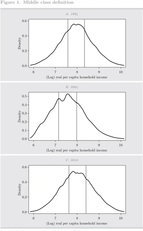
(14) 302. 4.. LATIN AMERICAN JOURNAL OF ECONOMICS | Vol. 50 No. 2 (Nov, 2013), 289–326. Data and results. We use the annual National Household Survey (ECH) conducted yearly by the National Statistical Of fice of Uruguay (INE).We employ cross-sectional data for 1994, 2004 and 2010 to analyze two dif ferent periods, 1994-2004 and 2004-2010. The first period is characterized by increasing inequality and it comprises the 2002 economic downturn6, while in the second one redistributive policies were introduced and average yearly real GDP growth was 6%. The ECH is the main source of socioeconomic information on Uruguayan households and their members at the national level. Because the 1994 and 2004 surveys only include households in urban areas with more than 5,000 inhabitants, we restrict the analysis to this population.7 We are interested in the total household income variable of the survey. This variable includes all sources of income (salaries, pensions, benefits from cash transfer programs, etc.) as well as imputed income (for example, in the case of homeowners, the imputed rental income is the hypothetical value that household members would have to pay for it). It is necessary to point out that the household income reported in the survey is net of social security and income taxes. Specifically, our outcome variable is the per-capita household income in March 1997 Uruguayan pesos since we adjust it by the consumer price index with base in March 1997.. 4.1 Characterizing the middle class In this section, we define and characterize the middle class following Esteban and Ray (1994) and then compare it with the other social classes (lower and upper). In Figure 1, we observe the density of the (log) real household income jointly with the middle class boundaries in 1994, 2004 and 2010. In 1994 and 2010 the definition seems to be quite similar, while in 2004 the middle-class interval shifts to the left, probably due to the 2002 economic crisis. Based on these middle-class intervals, Table 1 shows summary statistics of the middle classes. First of all, we observe that in Uruguay around 37% of the households belong to the middle class. The low-income class is the largest, with approximately 45%, and the upper class is the smallest (around 12%). Therefore, Uruguay is basically comprised 6. Real GDP decreased 11% in 2002 and unemployment reached 17% that year. 7. Note that only around the 5% of the Uruguay population is located in rural areas..

(15) F. Borraz, N. González, and M. Rossi | POLARIZATION AND THE MIDDLE CLASS IN URUGUAY. Figure 1. Middle class definition A. 1994. Density. 0.6. 0.4. 0.2. 0.0 6. 7 8 9 (Log) real per capita household income. 10. B. 2004. 0.5. Density. 0.4 0.3 0.2 0.1 0.0 6. 7 8 9 (Log) real per capita household income. 10. C. 2010. Density. 0.6. 0.4. 0.2. 0.0 6. 7 8 9 (Log) real per capita household income. Source: Authors’ computations based on data from ECH.. 10. 303.

(16) 6.05 10.34 0.59. % head of hhld with university degree. 2.97. % head of hhld with high school degree. 12.02. % households in [10,12]. % households in >12. Head of hhld years of education. 32.85. % households in [7,9]. 6.47 51.98. % households in < 7. Average household education. Education. 1.56. % of hhs below the extreme poverty line. 2.79. 20.44. 7.41. 11.27. 21.34. 28.58. 38.80. 7.85. 0.00. 0.00. 60.28. 61.67 29.69. % of labor income. % of hhs below the poverty line. 37.26. 25.68. 4.578 1.002. Household income share. 1.977 716.72. Average (per capita) household income. 37.26. Standard deviation. 54.17 44.57. % of persons. 32.50. 1994 Middle. Low. % of households. Variables. 15.59. 47.47. 10.74. 36.16. 28.70. 18.26. 16.88. 10.8. 0.00. 0.00. 60.1. 37.06. 6.134. 11.427. 18.17. 13.33. High. 0.65. 9.51. 7.17. 5.25. 20.36. 38.02. 36.36. 7.56. 4.66. 57.33. 60.06. 23.14. 520. 1.346. 46.42. 58.29. Low. Table 1. Characteristics of social classes: summary statistics 2004. 5.23. 28.14. 8.94. 21.56. 27.77. 23.08. 27.59. 9.24. 0.00. 0.00. 58.17. 35.33. 794. 3.396. 36.95. 30.16. Middle. 24.19. 62.9. 12.60. 54.36. 24.53. 10.04. 11.08. 12.50. 0.00. 0.00. 57.21. 41.53. 5.859. 9.252. 16.62. 11.56. High. 0.28. 8.34. 7.30. 4.94. 19.97. 40.36. 34.73. 7.59. 1.11. 27.72. 58.88. 26.01. 751. 2.103. 45.45. 56.62. Low. 2010. 3.01. 28.24. 9.38. 23.07. 29.99. 23.75. 23.19. 9.61. 0.00. 0.00. 60.96. 37.03. 1.115. 4.975. 37.15. 31.37. Middle. 16.04. 61.23. 12.80. 55.22. 25.65. 9.88. 9.25. 12.80. 0.00. 0.00. 59.15. 36.96. 8.782. 12.891. 17.40. 12.01. High. 304 LATIN AMERICAN JOURNAL OF ECONOMICS | Vol. 50 No. 2 (Nov, 2013), 289–326.

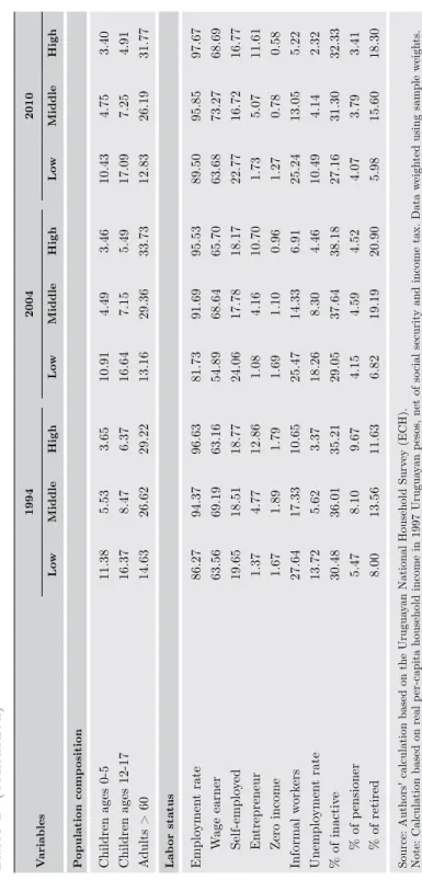
(17) 1994. 43.16. % of children in [7,15] with education gap. 3.92. Household size. 0.22. 0.14 -0.80. 97.22 44.62. Water supply - general network. Network evacuation. Asset index. 30.60. % of overcrowded households. Wealth Index. 69.90. 2.07. 2.81. 0.10. 98.44. 7.05. 1.45. 59.91. Homeownership. 73.27. 25.69. Persons per room. Living conditions. 0.76. 0.37. 42.46. 20.95. Average education gap - children in [7,15]. [18,23]. 86.56. 98.23 68.86. 99.78. Middle. [6,12]. Low. [13,17]. Attendance rate by age interval:. Variables. Table 1. (continued). 2.34. 1.22. 0.33. 91.08. 99.43. 1.32. 1.18. 81.05. 26.48. 0.32. 61.83. 94.47. 99.53. High. 3.83. -1.14. 0.17. 52.91. 98.24. 27.02. 2.00. 57.88. 46.64. 0.76. 33.59. 82.83. 98.34. Low. 2004. 2.52. 0.33. 0.29. 78.07. 99.22. 3.64. 1.38. 71.24. 27.00. 0.34. 64.99. 95.84. 99.23. Middle. 2.15. 1.60. 0.42. 92.50. 99.75. 0.93. 1.20. 81.17. 26.68. 0.31. 83.05. 99.45. 99.14. High. 3.54. -1.04. 0.24. 48.74. 98.17. 22.66. 1.87. 54.38. 47.22. 0.73. 28.42. 80.56. 98.88. Low. 2010. 2.40. 0.40. 0.33. 71.90. 98.95. 2.74. 1.28. 63.65. 29.02. 0.34. 55.85. 95.09. 99.12. Middle. 1.95. 1.70. 0.44. 87.15. 99.57. 0.37. 1.03. 71.65. 28.69. 0.33. 77.55. 98.68. 99.51. High. F. Borraz, N. González, and M. Rossi | POLARIZATION AND THE MIDDLE CLASS IN URUGUAY. 305.

(18) 14.63. Adults > 60. 13.56. 8.10. 36.01. 5.62. 17.33. 18.51. 11.63. 9.67. 35.21. 3.37. 10.65. 1.79. 12.86. 18.77. 63.16. 96.63. 29.22. 6.37. 3.65. High. 6.82. 4.15. 29.05. 18.26. 25.47. 1.69. 1.08. 24.06. 54.89. 81.73. 13.16. 16.64. 10.91. Low. 19.19. 4.59. 37.64. 8.30. 14.33. 1.10. 4.16. 17.78. 68.64. 91.69. 29.36. 7.15. 4.49. Middle. 2004. 20.90. 4.52. 38.18. 4.46. 6.91. 0.96. 10.70. 18.17. 65.70. 95.53. 33.73. 5.49. 3.46. High. 5.98. 4.07. 27.16. 10.49. 25.24. 1.27. 1.73. 22.77. 63.68. 89.50. 12.83. 17.09. 10.43. Low. 15.60. 3.79. 31.30. 4.14. 13.05. 0.78. 5.07. 16.72. 73.27. 95.85. 26.19. 7.25. 4.75. Middle. 2010. 18.30. 3.41. 32.33. 2.32. 5.22. 0.58. 11.61. 16.77. 68.69. 97.67. 31.77. 4.91. 3.40. High. Source: Authors' calculation based on the Uruguayan National Household Survey (ECH). Note: Calculation based on real per-capita household income in 1997 Uruguayan pesos, net of social security and income tax. Data weighted using sample weights.. 5.47 8.00. % of pensioner. % of retired. 13.72 30.48. Unemployment rate. % of inactive. 1.89. 1.67 27.64. Zero income. 1.37. Informal workers. 4.77. 19.65. Self-employed. Entrepreneur. 69.19. 86.27 63.56. Wage earner. 94.37. 26.62. 8.47. 5.53. Middle. 1994. Employment rate. Labor status. 11.38 16.37. Children ages 0-5. Low. Children ages 12-17. Population composition. Variables. Table 1. (continued). 306 LATIN AMERICAN JOURNAL OF ECONOMICS | Vol. 50 No. 2 (Nov, 2013), 289–326.

(19) F. Borraz, N. González, and M. Rossi | POLARIZATION AND THE MIDDLE CLASS IN URUGUAY. 307. of low- and middle-income households. Another interesting feature we observe is a great income dispersion in the upper class, while the lower class appears to be more homogeneous. Also, the income share of the middle and upper classes seems to be similar between 1994 and 2010, despite their size dif ferences. As expected, the income share of the lower class decreases in 2004, while that of the upper class increases. We present a second group of indicators that are related to education. Overall, we observe that educational attainment increases from the lower to the upper class. For instance, if we consider the average years of education of adult household members, the upper class has the highest average while the lower class has the lowest8. The attendance rate is similar across classes for the age cohort [6, 12]9. However, when we take into account higher cohorts the attendance rate decreases, mainly in the lower class case. In addition, the lower class shows a high education gap in children between 7 and 15 years old in comparison with the middle and upper class, which have a similar education gap. Regarding living conditions, around 70% of the middle-class households own their homes. Nevertheless, it is interesting to note that this proportion has declined in recent years and around 64% are homeowners in 2010. This trend is also evident in the other social classes. In addition, there is a considerable dif ference in terms of overcrowded households between the lower and the middle and the upper classes. Sanitation is another variable that increases as we move to higher-income classes. We construct an asset index as a weighted average of a series of indicator variables for the availability of the following household assets: refrigerator, dishwasher, washing machine, broadcast TV, Internet connection, computer, car and household help. The weights are the relative distance between 1 and the proportion of households having this item and therefore the index places more weight on items possessed only by few households. The index varies between 0 and 1. The asset index shows a dif ference between the low and middle classes of around 0.10 point and this gap remains constant for the three years. The asset gap between the middle and upper class is wider (approximately 0.14). We construct another wealth index with the same variables but considering a normal, standardized transformation of them. In this case, we observe larger gaps and this index varies among a higher set of values than before. 8. The same conclusion arises when we consider the average years of education of the head of household. 9. This is not surprising since primary school attendance is almost universal..

(20) 308. LATIN AMERICAN JOURNAL OF ECONOMICS | Vol. 50 No. 2 (Nov, 2013), 289–326. In regard to population composition, the lower class is comprised of more younger people than the other classes, while the middle and upper classes have more adults older than 60. The labor status indicators show that the unemployment rate is the highest for the lower-income class. The majority of the middleclass workers are wage earners, followed by the self-employed and then entrepreneurs. This pattern is quite similar in the other class categories. The major dif ference is that the high-income class has a greater proportion of workers in the entrepreneur category. We use the definition of informal workers adopted by the International Labour Organization at the 15th International Conference of Labor Statisticians (1993), which considers informal workers as those who work in the housekeeping sector, unpaid household members, private wage earners working in firms with less than five employees and selfemployed workers (excluding administrative workers, professionals and technicians). Using this definition, the highest proportion of informal workers is in the low-income class. The proportion of informal workers in the middle class in 1994 is just over 0.17 and decreases in both 2004 and 2010. Finally, the middle and upper classes show a similar share of inactive people. Table 2 presents multinomial logit estimates for the three years. As a dependent variable we use the category variable, which takes the value of 1 if the household belongs to the low-income category, 2 if it belongs to the middle and 3 if belongs to the high-income category. We consider the middle class as the base category and we report the marginal ef fects. It is interesting to note that the signs of the coef ficients do not change when we consider dif ferent years and that almost all the coef ficients are statistically dif ferent from zero at the 1% level. For instance, the probability of being a low-income household (with respect to being a middle-income household) decreases if the household is in the capital city (Montevideo). The opposite occurs when we analyze the probability of being a high-income household. This could be associated with dif ferences in the cost of living between the capital and the rest of the country. As mentioned earlier, households with young children have higher probabilities of being low-income than middle-class. The same holds for the household size variable. A more educated head of household raises the probability of being high-income and decreases the probability of being low-income (with respect to the middle). Concerning labor market variables, a head of household who is unemployed or works in the informal sector increases the probability.

(21) -0.132*** (0.007). 0.080*** (0.009). 0.094*** (0.008). -0.047*** (0.008). 0.083*** (0.003). -0.017*** (0.001). 0.190*** (0.022). -0.111*** (0.016). 0.032*** (0.007). -0.094*** (0.007). Household with children ages 0-5. Household with children ages 12-17. Household with adults > 60. Household size. Head of hhld average education. Head of hhld unemployed. Head of hhld occupation: entrepreneur. Households with informal workers. Homeownership. Low. Capital. Variables. Table 2a. Multinomial logit estimates 1994. 0.059*** (0.006). -0.040*** (0.007). 0.072*** (0.008). -0.069*** (0.020). 0.015*** (0.001). -0.075*** (0.003). 0.019*** (0.006). -0.042*** (0.007). -0.048*** (0.008). 0.074*** (0.006). High. -0.043*** (0.007). 0.025*** (0.007). -0.099*** (0.018). 0.153*** (0.015). -0.018*** (0.001). 0.098*** (0.003). -0.055*** (0.008). 0.078*** (0.008). 0.051*** (0.008). -0.044*** (0.007). Low. 2004. 0.046*** (0.006). -0.030*** (0.008). 0.079*** (0.009). -0.118*** (0.020). 0.016*** (0.001). -0.073*** (0.003). 0.038*** (0.006). -0.027*** (0.008). -0.031*** (0.009). 0.055*** (0.006). High. -0.048*** (0.004). 0.052*** (0.005). -0.083*** (0.011). 0.134*** (0.013). -0.022*** (0.001). 0.111*** (0.002). -0.041*** (0.006). 0.099*** (0.005). 0.075*** (0.006). -0.028*** (0.005). Low. 2010. 0.046*** (0.004). -0.052*** (0.005). 0.072*** (0.006). -0.081*** (0.014). 0.016*** (0.000). -0.088*** (0.002). 0.015*** (0.004). -0.034*** (0.005). -0.032*** (0.006). 0.037*** (0.004). High. F. Borraz, N. González, and M. Rossi | POLARIZATION AND THE MIDDLE CLASS IN URUGUAY. 309.

(22) -0.080*** (0.003). Wealth index. 11,906. Observations. 1994. 11,906. -7,678.08. 0.374. 0.050*** (0.002). 0.051*** (0.007). -0.042*** (0.016). High. Marginal ef fects and robust standard errors reported. Base category = middle class * significant at 10%; ** significant at 5%; *** significant at 1%.. -7,678.08. Log Likelihood. 0.374. -0.060*** (0.007). Network evacuation. Pseudo R2. 0.060*** (0.010). Low. Overcrowded households. Variables. Table 2a. (continued). 11,748. -7,064.40. 0.414. -0.078*** (0.002). -0.032*** (0.008). 0.047*** (0.012). Low. 2004. 11,748. -7,064.40. 0.414. 0.049*** (0.002). 0.005 (0.009). -0.032* (0.019). High. 27,914. -17,023.34. 0.395. -0.071*** (0.001). -0.044*** (0.005). 0.031*** (0.009). Low. 2010. 27,914. -17,023.34. 0.395. 0.046*** (0.001). 0.017*** (0.005). -0.050*** (0.019). High. 310 LATIN AMERICAN JOURNAL OF ECONOMICS | Vol. 50 No. 2 (Nov, 2013), 289–326.

(23) F. Borraz, N. González, and M. Rossi | POLARIZATION AND THE MIDDLE CLASS IN URUGUAY. 311. Table 2b. Ordered logit estimates 1994 Middle. 2004 Middle. 2010 Middle. Capital. 0.042*** (0.002). 0.015*** (0.002). 0.012*** (0.001). Household with children ages 0-5. -0.026*** (0.003). -0.013*** (0.002). -0.021*** (0.002). Household with children ages 12-17. -0.028*** (0.002). -0.018*** (0.002). -0.026*** (0.001). Household with adults > 60. 0.013*** (0.002). 0.015*** (0.002). 0.010*** (0.001). Household size. -0.030*** (0.001). -0.027*** (0.001). -0.035*** (0.001). Head of hhld average education. 0.007*** (0.000). 0.006*** (0.000). 0.007*** (0.000). Head of hhld unemployed. -0.056*** (0.007). -0.043*** (0.004). -0.040*** (0.004). Head of hhld occupation: entrepreneur. 0.035*** (0.004). 0.028*** (0.003). 0.029*** (0.002). Households with informal workers. -0.013*** (0.002). -0.008*** (0.002). -0.017*** (0.001). Homeownership. 0.031*** (0.002). 0.014*** (0.002). 0.017*** (0.001). Overcrowded households. -0.015*** (0.003). -0.012*** (0.003). -0.007*** (0.003). Network evacuation. 0.021*** (0.002). 0.007*** (0.002). 0.012*** (0.001). Wealth index. 0.025*** (0.001). 0.021*** (0.001). 0.021*** (0.000). Variables. Pseudo R 2 Log Likelihood Observations. 0.368. 0.413. 0.393. -7,756.56. -7,077.75. -17,140.93. 11,906. 11,748. 27,914. Marginal ef fects and robust standard errors reported. Base category = middle class * significant at 10%; ** significant at 5%; *** significant at 1%.. of being low-income, while decreasing the probability of being highincome. In addition, if the head of household is an entrepreneur, this increases the probability of being high-income. The housing variables have the expected signs. Because in this case the dependent variable seems to have a natural order, an ordered logit model appears to be the most appropriate. However, if this assumption does not hold we will have a bias estimator. Otherwise, the ordered logit model produces more ef ficient estimates.

(24) 312. LATIN AMERICAN JOURNAL OF ECONOMICS | Vol. 50 No. 2 (Nov, 2013), 289–326. than the multinomial logit. However, the results of both models are quite similar, so we do not report the ordered logit estimation.10. 4.2.. Evolution of the middle class and polarization. In this section, we apply the methodology related to the evolution of the middle class and the polarization measures. Table 3 presents summary statistics that help describe the income distribution for the different years. As we can see, the mean and the median of the income distribution fall between 1994 and 2004 and both increase in 2010. The mean is greater than the median, indicating that the income distribution is skewed left. With respect to income concentration, the first quintile has approximately 5% of the total income, while the fifth quintile represents approximately 50%. Interestingly, during the first period the proportion of the first quintile declines, whereas that of the fifth rises. In the second period we observe the opposite pattern. This also can be viewed in the income share measures. The bottom five percentile has an income share of just under 1%, which decreases in the first period and subsequently increases. The top five percentile has an income share of 20% in 1994, which rises one percentage point and then declines to just over 20%. The next group of indicators measures the population share given a specific income range. For instance, we observe that 10% of households have income less than 40% of the median in 1994, and so on. Considering low and high income values as a percentage of the median, we observe that the population share grows in the first period and in the subsequent period it drops. However, if we consider income intervals near or around the median this trend reverses. This generates the perception of a decrease in the middle class during the 1994-2004 period, and an increase in the next period. Using the M curve, this perception is confirmed. The middle class decreases by around 3% in the 1994-2004 period (the movement from the middle was both upward and downward), and then rises by 2 percentage points in the following period. When analyzing different population ranges around the middle, we also observe that a larger income spread is required to capture those ranges in 2004, reflecting greater income variation in the income distribution in that year. For example, given a population range between 20% and 80%, we require an income spread of 141% of the median income in 2004. This percentage falls by 8% in 2010. 10. The results are available from the authors upon request..

(25) 14.99. 21.96. 47.12. 2sd Quantile. 3rd Quantile. 4th Quantile. 5th Quantile. 0.78. 2.07. 5.60. 47.13. 30.84. 19.69. Bottom 5%. Bottom 10%. Bottom 20%. Top 20%. Top 10%. Top 5%. Income share (%). 5.61. 10.32. 1st Quantile. Quintiles (%). 74.53. 3,476.21. Median. Median/mean. 4,664.18. Mean. Centrality measures. 1994 (1). 21.65. 33.15. 49.47. 4.94. 1.83. 0.71. 53.80. 20.69. 13.03. 8.27. 4.22. 71.43. 2,409.77. 3,373.71. 2004 (2). 20.46. 31.61. 47.83. 5.50. 2.07. 0.81. 49.37. 21.50. 14.34. 9.63. 5.17. 73.35. 3,669.35. 5,002.64. 2010 (3). 22.14. 33.79. 50.19. 4.85. 1.82. 0.71. 54.54. 20.43. 12.86. 8.04. 4.14. 70.09. 2,286.45. 3,262.06. 2004a (4). 22.13. 32.52. 48.95. 5.16. 1.94. 0.77. 50.49. 21.40. 14.04. 9.18. 4.88. 71.88. 3,444.06. 4,791.46. 2010b (5). Table 3. Description of income distribution and middle class measures. 1.96. 2.31. 2.34. -0.66. -0.24. -0.07. 2.34. -0.22. -0.61. -0.85. -0.66. -3.10. -1,066.44. -1,290.47. Difference (2) - (1). -1.19. -1.54. -1.64. 0.56. 0.24. 0.10. -4.43. 0.81. 1.31. 1.36. 0.95. 1.92. 1,259.58. 1,628.91. Difference (3) - (2). -0.01. -1.27. -1.24. 0.31. 0.12. 0.06. -4.05. 0.97. 1.18. 1.14. 0.74. 1.79. 1,157.61. 1,529.40. Difference (5) - (4). F. Borraz, N. González, and M. Rossi | POLARIZATION AND THE MIDDLE CLASS IN URUGUAY. 313.

(26) (continued). 16.61. 23.41. 10.76. 15.82. 12.71. 8.80. 17.57. < 60% of median. 60% to 75%. 75% to 100%. 100% to 125%. 125% to 150%. > 200%. 37.33. 28.53. 54.90. 75% to 150% of median. 75% to 125%. 50% to 150%. % in M-curve given income range. 10.38. < 50% of median. 1994 (1). < 40% of median. % of Population with income:. Table 3.. 50.64. 25.78. 34.57. 18.60. 8.79. 11.24. 14.54. 9.26. 26.20. 19.39. 12.68. 2004 (2). 53.82. 27.20. 36.19. 17.78. 8.99. 11.93. 15.28. 10.58. 24.14. 17.10. 10.71. 2010 (3). 49.82. 25.22. 33.73. 19.28. 8.51. 10.88. 14.34. 9.27. 26.38. 19.56. 12.81. 2004a (4). 51.99. 25.76. 34.59. 18.75. 8.83. 11.38. 14.38. 10.28. 25.35. 18.22. 11.90. 2010b (5). -4.26. -2.75. -2.76. 1.03. -0.01. -1.47. -1.28. -1.50. 2.79. 2.78. 2.30. Difference (2) - (1). 3.18. 1.42. 1.62. -0.82. 0.20. 0.69. 0.74. 1.32. -2.06. -2.29. -1.97. Difference (3) - (2). 2.17. 0.54. 0.86. -0.53. 0.32. 0.50. 0.04. 1.01. -1.03. -1.34. -0.91. Difference (5) - (4). 314 LATIN AMERICAN JOURNAL OF ECONOMICS | Vol. 50 No. 2 (Nov, 2013), 289–326.

(27) (continued). 54.34. 75.30. 100.47. 131.25. 30% to 70%. 25% to 75%. 20% to 80%. 1.011. 1.021. 1.036. 1.057. 18.386. 35% to 65%. 30% to 70%. 25% to 75%. 20% to 80%. Observations. 18.392. 1.078. 1.051. 1.033. 1.019. 1.009. 141.30. 109.91. 83.80. 60.38. 39.92. 2004 (2). 40.539. 1.064. 1.042. 1.025. 1.014. 1.007. 133.23. 103.67. 79.08. 57.22. 37.23. 2010 (3). 18.392. 1.083. 1.055. 1.036. 1.020. 1.009. 144.78. 113.47. 86.08. 62.24. 40.87. 2004a (4). 40.539. 1.068. 1.044. 1.025. 1.013. 1.005. 140.30. 109.12. 82.57. 60.20. 39.26. 2010b (5). 0.021. 0.015. 0.012. 0.008. 0.003. 10.05. 9.44. 8.50. 6.04. 4.34. Difference (2) - (1). -0.014. -0.009. -0.008. -0.005. -0.002. -8.07. -6.24. -4.72. -3.16. -2.69. Difference (3) - (2). -0.015. -0.011. -0.011. -0.007. -0.004. -4.48. -4.35. -3.51. -2.04. -1.61. Difference (5) - (4). Source: Authors' calculation based on the Uruguayan National Household Survey (ECH). Note: Calculation based on the real per capita household income in March 1997 Uruguayan pesos, net of social security and income tax. Income data weighted using sample weights. a household income without considering the old health system (OHS) income. b household income without considering the new health system (NHS) income.. 1.006. 40% to 60%. Avg distance given pop range:. 35.58. 35% to 65%. 1994 (1). 40% to 60%. S given pop range:. Table 3.. F. Borraz, N. González, and M. Rossi | POLARIZATION AND THE MIDDLE CLASS IN URUGUAY. 315.

(28) 316. LATIN AMERICAN JOURNAL OF ECONOMICS | Vol. 50 No. 2 (Nov, 2013), 289–326. Figure 2. Middle class and polarization curves A. Evolution of the middle class; M-curve 0.5. 0.5. 0.4. 0.4. 0.3. 0.3. 0.2. 0.2. 0.1. 0.1. 0.0. 0.0. 0.5. 1.0 std income. 1.5. 2.0. 0.0. 0.0. 0.5. 1.0 std income. 1.5. 2.0. 0.6. 0.8. B. Evolution of polarization; S - first degree curve 1.5. 1.5. 1.0. 1.0. 0.5. 0.5. 0.0. 0.0. 0.2. 0.4. 0.6. 0.8. 0.0. 1994. 0.0. 0.2. 0.4. 2004. Source: Authors’ computations based on data from ECH.. All of these observed features are illustrated in Figure 2. In the top panels we plot the M-curve, which measures the concentration of mass around the median of the income distribution. We observe that the M-curve of the income distribution of 1994 is above the M-curve of the income distribution of 2004 (and they do not cross each other), and thus Proposition 1 holds: “The income distribution function in 1994 has an unambiguously larger middle class than the income distribution function in 2004.” In other words, the 1994 income distribution has more mass around the median than the 2004 income distribution. Moreover, the first- and second-degree polarization curves (middle and lower panels) lead to the same conclusions as before. Those latter curves indicate that polarization in the income distribution in 2004 is higher than polarization in the income distribution in 1994, revealing that the latter has a greater income spread. Since a greater income spread implies a lower proportion of population around the middle, according to Proposition 3 the 1994 income distribution has a larger middle class than the 2004 income distribution and therefore, the former.

(29) F. Borraz, N. González, and M. Rossi | POLARIZATION AND THE MIDDLE CLASS IN URUGUAY. 317. dominates the latter. Additionally, the second-degree polarization curve in 1994 is below the second-degree polarization curve in 2004, which implies that the income distribution in 2004 has a greater spread, as well as a greater bipolarity than the income distribution in 1994. The second period, 2004-2010, shows the opposite picture. The middle class increases while polarization tends to decline. Table 4 contains inequality and polarization indices. The inequality indicators show a sharp increase between 1994 and 2004. For instance, the Gini index rises from 0.409 to 0.439. The generalized entropy index, the Atkinson index and the coefficient of variation index increase 0.054, 0.021 and 0.143 points, respectively. As mentioned above, this period is characterized by a tendency toward increasing inequality which is enhanced by the economic downturn that began in the late 1990s. This period of growing inequality is also accompanied by a significant rise in income polarization. The Duclos et al. index grows around 0.015 for dif ferent levels of identification represented by the parameter α. That is, for dif ferent values of α, the change in the Duclos et al. index between 1994 and 2004 is statistically dif ferent from zero at the 1% level. A greater value of α means that more emphasis is placed on the identification process. In order to analyze the contribution of each of the sources of polarization, the index can be decomposed into three (multiplicative) components: identification, alienation (which is equal to the Gini index) and correlation (between the two measures). It is interesting to note that while the alienation and correlation components evolve positively, the identification component declines. This result holds for dif ferent values of the α parameter. In other words, polarization basically increases because the gap between the identified groups rises. For the second period, 2004-2010, the first main result is a decline in inequality. With the exception of the coefficient of variation index, the reduction is statistically different from zero. The second interesting result is that, as we have already noted, polarization falls. If we focus on the Duclos et al. (2004) index, the magnitude of the reduction decreases with the value of the α parameter. This can be explained by the fact that we give the greatest weight to the identification effect, which in this case goes in the opposite direction. Despite polarization declining slightly, the identification component rises but not enough to offset the reduction of the alienation effect. The Foster and Wolfson polarization measure deserves a very similar reading. In the first period, we observe a statistically significant increase in the bipolarization index. In this case, we observe an.

(30) 0.158 (0.002) 1.077 (0.038). 0.136 (0.002). 0.934 (0.016). Atkinson index. Coefficient of variation index. 0.884 0.258 (0.001) 0.837 0.222 (0.001). 0.834. 0.877. 0.243 (0.001). 0.725. 0.819. 0.209 (0.001). 0.646. 0.791. Identification. Correlation. α = 0.50. Identification. Correlation. α = 0.75. Identification. Correlation. 0.814. 0.621. 0.702. 0.817. 0.299 (0.001). α = 0.25. Duclos, Esteban and Ray (polarization) Index 0.317 (0.002). 0.353 (0.008). 0.298 (0.005). Generalized entropy index. Polarization. 0.439 (0.003). 2004 (2). 0.409 (0.003). 1994 (1). 0.797. 0.645. 0.215 (0.001). 0.824. 0.723. 0.249 (0.001). 0.878. 0.831. 0.305 (0.001). 1.049 (0.039). 0.143 (0.002). 0.321 (0.011). 0.418 (0.002). 2010 (3). Polarization and inequality measures. Gini index. Inequality. Table 4.. 0.809. 0.625. 0.226 (0.002). 0.833. 0.704. 0.262 (0.001). 0.881. 0.818. 0.322 (0.002). 1.106 (0.040). 0.163 (0.003). 0.366 (0.008). 0.447 (0.003). 2004a (4). 0.797. 0.642. 0.221 (0.001). 0.823. 0.720. 0.256 (0.001). 0.877. 0.829. 0.314 (0.001). 1.092 (0.040). 0.152 (0.002). 0.343 (0.007). 0.432 (0.002). 2010b (5). 0.013***. 0.015***. 0.018***. 0.143***. 0.021***. 0.054***. 0.030***. Difference (2) - (1). -0.007***. -0.009***. -0.013***. -0.028. -0.015***. -0.032***. -0.021***. Difference (3) - (2). -0.005***. -0.006***. -0.008***. -0.013. -0.011***. -0.023**. -0.015***. Difference (5) - (4). 318 LATIN AMERICAN JOURNAL OF ECONOMICS | Vol. 50 No. 2 (Nov, 2013), 289–326.

(31) (continued). 18.392. 40.539. 0.278. 0.140. 0.188. 0.555. 2010 (3). 0.296. 0.151. 0.206. 0.591. 2004a (4). 0.287. 0.145. 0.197. 0.574. 2010b (5). 0.019***. 0.011***. 0.018***. 0.037***. Difference (2) - (1). -0.014***. -0.008***. -0.012***. -0.014***. Difference (3) - (2). -0.009***. -0.006***. -0.009***. -0.017***. Difference (5) - (4). Source: Authors' calculation based on the Uruguayan National Household Survey (ECH). Note: Calculation based on the real per capita household income in March 1997 Uruguayan pesos, net of social security and income tax. Income data weighted using sample weights. a household income without considering the old health system (OHS) income. b household income without considering the new health system (NHS) income. * significant at 10%; ** significant at 5%; *** significant at 1%.. 18.386. Observations. 0.291. 0.148. 0.137. 0.272. Within gini index. Between gini index. 0.200. 0.545. 0.182. 0.582. 2004 (2). Relative median deviation. 1994 (1). Bipolarization Index. Foster & Wolfson. Table 4.. F. Borraz, N. González, and M. Rossi | POLARIZATION AND THE MIDDLE CLASS IN URUGUAY. 319.

(32) 320. LATIN AMERICAN JOURNAL OF ECONOMICS | Vol. 50 No. 2 (Nov, 2013), 289–326. Figure 3. Actual and relative density A. Reference group 1994; comparison group 2004 4 Relative density. Density. 0.6 0.4 0.2. 3 2 1. 0.0. 0 6. 7 8 9 (Log) real per capita income. 10. 0.0. 0.2 0.4 0.6 0.8 Proportion of reference group. 1.0. B. Reference group 2004; comparison group 2010 2.5. Relative density. Density. 0.6 0.4 0.2 0.0. 2.0 1.5 1.0 0.5 0.0. 6. 7 8 9 (Log) real per capita income. 10. Actual density 2004. 0.0. 0.2 0.4 0.6 0.8 Proportion of reference group. 1.0. Actual density 2010. Source: Authors’ computations based on data from ECH.. increase in inequality within and between the two groups.11 Therefore, both groups spread out and the distance between them increases (“increased spread” and “increased bipolarity”). In the second period, the reduction in the within- and the between-Gini indices indicates a decreases in polarization. We apply the relative distribution approach in order to find changes in the entire income distribution. Figure 3 shows the actual income distribution in 1994 and 2004 in the left plot and the relative distribution in the right plot of the top panel. At first glance, there is a shift from the right to the left which implies a reduction of mean income in this period. On the contrary, we observe a shift from the. 11. As previously mentioned, Foster and Wolfson identify only two groups, those above and those below the median of the income distribution..

(33) F. Borraz, N. González, and M. Rossi | POLARIZATION AND THE MIDDLE CLASS IN URUGUAY. 321. Figure 4. Location and shape effects A. Reference group 1994; comparison group 2004 Shape effect. 2.5. 2.5. 2.0. 2.0. Relative density. Relative density. Location effect. 1.5 1.0 0.5 0.0. 1.5 1.0 0.5 0.0. 0.0. 0.2 0.4 0.6 0.8 Proportion of reference group. 1.0. 0.0. 0.2 0.4 0.6 0.8 Proportion of reference group. 1.0. B. Reference group 2004; comparison group 2010 Location effect. Shape effect 4 Relative density. Relative density. 4 3 2 1 0. 3 2 1 0. 0.0. 0.2 0.4 0.6 0.8 Proportion of reference group. 1.0. 0.0. 0.2 0.4 0.6 0.8 Proportion of reference group. 1.0. Source: Authors’ computations based on data from ECH.. left to the right in the income distribution during the 2004-2010 period (see lower panel of Figure 3). In Figure 4, we observe the location and the shape ef fect. The plots on the left confirm our prior observation since we find a decreasing and increasing location ef fect for the first and second periods, respectively. The right (top) plot shows how the lower and upper tail of the income distribution increase during the 1994-2004 period. This fact supports prior findings concerning a decline around the middle of the income distribution. In the other period, the shape ef fect shows that the lower and upper tail decline and the middle increases slightly. To formalize this result, and based on the relative density, we calculate relative polarization measures where positive values mean that polarization increases. In fact, we observe positive values that are statistically dif ferent from zero for the three measures in the first period. In.

(34) 322. LATIN AMERICAN JOURNAL OF ECONOMICS | Vol. 50 No. 2 (Nov, 2013), 289–326. the second period, the three indices are negative. This means that polarization decreases, which is in line with our previous findings. However, the change is smaller than in the first period. To summarize, throughout the 1990s and until 2004 the income distribution becomes more unequally distributed and more polarized and the middle class shrinks considerably, while during the 2004-2010 period we observe some improvements.. 4.3. Robustness analysis In order to analyze the robustness of our results, we do not include as household income the health services derived from the new healthcare system (NHS) implemented in 2008.12 In the new scheme, children under 18 years old of formal employees automatically acquired the right to medical services and therefore are not subject to the monthly payment.13 The reform implies an important increase in the number of persons af filiated with private hospitals.14 The National Statistical Of fice of Uruguay (INE) accounts for this change by imputing a monthly payment for healthcare services to household income15. From a theoretical point of view, it is not clear whether this should include be included as income. If we do not impute this income, the results could change because the income distribution is sensitive to this imputation (mainly for low-income households). As we can see in Table 3 (fourth and fifth column) the proportion of income in the first and in the second quintiles decreases. What’s more, the percentage of households around the median drops while the proportions at the extremes tend to increase. This is confirmed in the summary statistics related to the M-curve. In the previous section, we conclude that the middle class increases. However, if we do not include the imputation for health reform as household income (as well as the imputed income for healthcare services to wage earners in 2004), the change in the middle is ambiguous. This situation is illustrated by Figure 5, where the M-curve of the income distribution of 2004 is still 12. For a complete discussion of the 2008 health reform see Bérgolo and Cruces (2010). 13. This change was financed with an increase in worker contributions. 14. According to the Ministry of Public Health, the number of customers of collective healthcare institutions, which are the main private healthcare suppliers, increased by 314,976 between December 2007 and December 2008. 15. The INE also includes in 2004 household income the amount accounting for the health services for each household member who is a wage earner..

(35) F. Borraz, N. González, and M. Rossi | POLARIZATION AND THE MIDDLE CLASS IN URUGUAY. 323. Figure 5. Robustness analysis A. Middle class curve M - curve 2004 M - curve 2010. 0.4. Cumulative spread. Population share. 0.5. C. Polarization curve. 0.3 0.2 0.1. 0.6. B - curve 2004 B - curve 2010. 0.4 0.2 0.0. 0.0 0.0. 0.5 1.0 1.5 Normalized income. 0.0. 2.0. C. Location effect. 0.4 0.6 Percentile. 0.8. 1.0. D. Shape effect 4 Relative density. 4 Relative density. 0.2. 3 2 1 0. 3 2 1 0. 0.0. 0.2 0.4 0.6 0.8 Proportion of reference group. 1.0. 0.0. 0.2 0.4 0.6 0.8 Proportion of reference group. 1.0. Source: Authors’ computations based on data from ECH.. below the M-curve of the income distribution of 2010, but around the middle both curves are quite similar. This result implies that the middle class increases. Nevertheless, around the middle its increment is not as pronounced as observed in the previous section. The same is also evident in the shape ef fect panel, in which the extreme poles seem to decline while the middle increases, but to a lesser extent than in the previous section. With respect to the polarization and inequality measures in Table 4, the various indicators decrease as before, but to a lesser extent. For instance, the Gini index decreases from 0.439 in 2004 to 0.418 in 2010 (0.021 points), while if we do not impute income for healthcare services the decline is 0.015. The same picture holds for the other indices where the changes are statistically dif ferent from zero, but with a lower change than in the original case. Furthermore, polarization grows for dif ferent values of the α parameter. In this case, the most important component of polarization is alienation since identification remains steady. Therefore, the higher the value of α, the lower the.

(36) 324. LATIN AMERICAN JOURNAL OF ECONOMICS | Vol. 50 No. 2 (Nov, 2013), 289–326. Table 5. Relative polarization measures 1994-2004 (1). 2004-2010 (2). 2004a-2010b (3). Median relative polarization index. 0.069*** (0.006). -0.052*** (0.005). -0.035*** (0.005). Lower relative polarization index. 0.076*** (0.010). -0.058*** (0.009). -0.041*** (0.009). Upper relative polarization index. 0.062*** (0.010). -0.045*** (0.009). -0.029* (0.009). Source: Authors' calculation based on the Uruguayan National Household Survey (ECH). Note: Calculation based on the real per capita household income in March 1997 Uruguayan pesos, net of social security and income tax. Income data weighted using sample weights. (1) Reference group 1994 and comparison group 2004; (2) reference group 2004 and comparison group 2010. a household income without considering the old health system (OHS) income. b household income without considering the new health system (NHS) income. * significant at 10%; ** significant at 5%; *** significant at 1%.. ef fect. The conclusions are the same with respect to the Foster and Wolfson indexes and relative polarization measures (Tables 4 and 5).. 5.. Concluding remarks. In recent years there has been increasing concern about inequality and polarization. The expansion of the middle class is one of the key issues contributing to a reduction in inequality and less polarization. From an economic and social perspective, the middle class could play an important role in the development of a democratic country because it contributes a significant share of the labor force, and therefore is closely related to the country’s output and usually represents the main source of tax revenue. Furthermore, an increase in the middle class resulting from reduction of the lower and upper classes could enhance the positive externalities mentioned above, decreasing income inequality and social tension. We analyze the middle class and polarization in Uruguay over the last two decades. We conclude that the middle class decreases in size and income polarization increases between 1994 and 2004, while the opposite occurs between 2004 and 2010. However, when we do not include the income imputation due to the health reform implemented in 2008, the results tend to be attenuated. In other words, the expansion of the middle class between 2004 and 2010 is reduced and the magnitude of the decline is af fected by the health income imputation, highlighting the importance of analyzing income imputation when using household surveys..

(37) F. Borraz, N. González, and M. Rossi | POLARIZATION AND THE MIDDLE CLASS IN URUGUAY. 325. References Aghion, P., E. Caroli, and C. Garcia-Penalosa (1999), “Inequality and economic growth: The perspective of the new growth theories,” Journal of Economic Literature 37(4): 1615–60. Amarante, V. and A. Vigorito (2006), “Evolución de la pobreza en el Uruguay,” Instituto Nacional de Estadística. Andersen, L.E. (2001), “Social mobility in Latin America: Links with adolescent schooling,” Research Network Working Papers R-433, Inter-American Development Bank. Azzimonti, M. (2011), “Barriers to investment in polarized societies,” American Economic Review 101(5): 2182–204. Banerjee, A.V. and E. Duflo (2008), “What is middle-class about the middle classes around the world?” Journal of Economic Perspectives 22(2): 3–28. Barro, R. (1999), “Determinants of democracy,” Journal of Political Economy 107(S6): S158–S183. Barriex, A. and J. Roca (2007) “Reforzando un pilar fiscal: El impuesto a la renta dual a la Uruguaya,” Revista de la CEPAL: 123–42. Bérgolo, M. and G. Cruces (2010), “Labor informality and the incentive ef fects of social security: Evidence from a health reform in Uruguay,” CEDLAS, Universidad Nacional de la Plata. Borraz, F. and N. González (2009), “The impact of the Uruguayan conditional cash transfer program,” Latin American Journal of Economics 46(134): 243–71. Bourguignon, F. and C. Morrison (2002), “Inequality among world citizens: 18201992,” American Economic Review 92: 727–43. Cruces, G., L.F. Lopez-Calva, and D. Battiston (2010), “Down and out or up and in? In search of Latin American´s elusive middle class,” Research for Public Policy, Inclusive Development, ID-03-2010, RBLAC-UNDP. Duclos, J., J. Esteban, and D. Ray (2004), “Polarization: concepts, measurements, Estimation,” Econometrica 72: 1737–72. Easterly, W. (2001). “The middle class consensus and economic development,” Journal of Economic Growth 6(4): 317–35. Esteban, J. and D. Ray (1994), “On the measurement of polarization,” Econometrica 62: 819–52. Foster, J. and M. Wolfson (2009), “Polarization and the decline of the middle class: Canada and the U.S.,” Journal of Economic Inequality 8(2): 247–73. Gasparini, L., E. Horenstein, E. Molina, and S. Olivieri (2008), “Income polarization in Latin America: Patterns and links with institutions and conflict,” Oxford Development Studies 36(4): 463–84. Goldthorpe, J. (1980), Social mobility and class structure in modern Britain. Oxford: Clarendon Press..