Multi phase resilience assessment and adaptation of electric power systems throughout the impact of natural disasters

Texto completo

(1)PONTIFICIA UNIVERSIDAD CATOLICA DE CHILE SCHOOL OF ENGINEERING. MULTI-PHASE RESILIENCE ASSESSMENT AND ADAPTATION OF ELECTRIC POWER SYSTEMS THROUGHOUT THE IMPACT OF NATURAL DISASTERS. SEBASTIAN ANDRES ESPINOZA. Thesis submitted to the Office of Research and Graduate Studies in partial fulfilment of the requirements for the Degree of Master of Science in Engineering Advisor: HUGH RUDNICK VAN DE WYNGARD. Santiago de Chile, October 2015. © MMXV, Sebastián Andrés Espinoza Lara.

(2) PONTIFICIA UNIVERSIDAD CATOLICA DE CHILE SCHOOL OF ENGINEERING. MULTI-PHASE RESILIENCE ASSESSMENT AND ADAPTATION OF ELECTRIC POWER SYSTEMS THROUGHOUT THE IMPACT OF NATURAL DISASTERS. SEBASTIAN ANDRES ESPINOZA. Members of the Committee: HUGH RUDNICK VAN DE WYNGARD DANIEL OLIVARES QUERO RODRIGO MORENO VIEYRA MIGUEL RIOS OJEDA. Thesis submitted to the Office of Research and Graduate Studies in partial fulfilment of the requirements for the Degree of Master of Science in Engineering. Santiago de Chile, October 2015..

(3) DEDICATION. To my loving sister, mother and grandmother.. ii.

(4) ACKNOWLEDGEMENTS I would like to express my deepest gratitude to my advisor, Professor Hugh Rudnick, not only for his constant support and guidance in the past years, but also because through his example he has shown me different ways to serve those around me. Special thanks to Mathaios Panteli and Professor Pierluigi Mancarella from The University of Manchester, who have been working in the Electric Power Systems group together with Tyndall Centre for Climate Change trying to tackle global problems. I am much obliged for the co-work and for receiving me in Manchester for a semester. Also thanks for the co-work to Felipe Rivera, Alan Poulos, Paula Aguirre, Jorge Vásquez, Juan Gonzáles and the dean Juan Carlos de la Llera from CIGIDEN, who are developing scientific knowledge that will enable Chile to be better prepared to confront natural disasters. My gratitude to Rodrigo Moreno from University of Chile for his kind academic and personal advises. Thanks to Óscar Alamos from the Ministry of Energy, Helia Molina from ONEMI, Mark Beswick from the MET UK Office, Jorge Araya from GSI and Juan Carlos Araneda, Raúl Moreno and Marco Quezada from CDEC-SING. Also my gratitude to Carlos Medel, Alejandro Navarro, Luis Gutierrez and Carlos Cruzat for having the time to answer my questions and all the people in The University of Manchester for making me feel at home. Thanks to the past and present friends of the Office 302, where we had endless days discussing how to solve the energy problems of the world. And of course, thanks for the constant support of my girlfriend Pía and my lifefriends. Thanks especially to my family for every little detail that have made me who I am. Thanks to all for all those afternoons that you gave to this project without thinking in what you would receive back. I finally hope this research is a small contribution to the disaster management and electric power systems fields. Chile and countries affected by major natural disasters need to improve their actions at the preparedness, response, recovery and mitigation stages while having a special care for those in need within the society, who are at the same time the most affected. ”Pray as though everything depended on God. Work as though everything depended on you”. - Saint Augustine iii.

(5) TABLE OF CONTENTS Page DEDICATION ............................................................................................................. ii ACKNOWLEDGEMENTS ........................................................................................ iii LIST OF FIGURES.................................................................................................... vii LIST OF TABLES ...................................................................................................... ix ABSTRACT ................................................................................................................. x RESUMEN .................................................................................................................. xi 1. INTRODUCTION............................................................................................... 12 1.1 Motivation ................................................................................................ 12 1.2 Objectives ................................................................................................. 12 1.3 Research delimitations ............................................................................. 13 1.4 General methodology ............................................................................... 15 1.5 Thesis outline ........................................................................................... 16 2. BASIC CONCEPTS............................................................................................ 17 2.1 Definitions ................................................................................................ 17 2.2 System’s performance curve throughout a disaster.................................. 18 2.3 Electric power system’s structure ............................................................ 19 2.4 Types of risk analyses .............................................................................. 20 3. STATE OF THE ART AND CONTRIBUTIONS OF THIS THESIS ............... 23 3.1 Different perspectives for the resilience concept ..................................... 23 3.2 Methodological advances of resilience assessment and adaptation in electric power systems ............................................................................. 24 3.3 Contributions of the present work ............................................................ 25 4. MULTI-PHASE RESILIENCE ASSESSMENT AND ADAPTATION FRAMEWORK ................................................................................................ 27 4.1 Multi-phase resilience assessment ........................................................... 27 4.1.1 Phase one: threat characterization.................................................. 28 .

(6) 4.1.2 Phase two: fragility of system’s components ................................ 30 4.1.3 Phase three: system’s reaction ....................................................... 32 4.1.4 Phase four: system’s restoration .................................................... 33 4.2 Multi-phase adaptation strategies ............................................................. 34 4.3 Resilience metrics .................................................................................... 35 4.4 Resilience modelling ................................................................................ 36 5. APPLICATION TO WINDSTORMS AND FLOODS IN GREAT BRITAIN . 37 5.1 Influence of extreme weather and climate change in Great Britain’s power system ............................................................................................ 37 . 5.2 5.3 . 5.4 5.5 . 5.1.1 Extreme weather events ................................................................. 37 5.1.2 Climate change and future hazard scenarios.................................. 38 The Great Britain’s simplified electric power system .............................. 39 Resilience assessment .............................................................................. 40 5.3.1 Phase one: windstorms and floods characterization ...................... 40 5.3.2 Phase two: fragility of electrical components ................................ 43 5.3.3 Phase three: power system’s reaction ............................................ 44 5.3.4 Phase four: power system’s restoration ......................................... 45 Resilience adaptation................................................................................ 46 Results and discussion .............................................................................. 47 . 6. APPLICATION TO EARTHQUAKES IN CHILE ............................................ 51 6.1 Influence of earthquakes and tsunamis in Chile....................................... 51 6.1.1 Influence of earthquakes in Chile’s power systems....................... 52 6.1.2 Future hazard scenarios in northern Chile ..................................... 54 6.2 The northern Chilean reduced electric power system .............................. 55 6.3 Resilience assessment .............................................................................. 58 6.3.1 Phase one: earthquakes characterization........................................ 58 6.3.2 Phase two: fragility of electrical components ................................ 59 6.3.3 Phase three: power system’s reaction ............................................ 62 6.3.4 Phase four: power system’s restoration ......................................... 64 6.4 Resilience adaptation................................................................................ 65 6.5 Results and discussion .............................................................................. 66 7. CONCLUSIONS ................................................................................................. 70 .

(7) 8. FUTURE WORK ................................................................................................ 72 REFERENCES ........................................................................................................... 74 A P P E N D I C E S................................................................................................... 82 APPENDIX A : CORRELATION BETWEEN ELECTRICITY CONSUMPTION AND ECONOMIC GROWTH ......................................................................... 83 APPENDIX B : MULTI-PHASE RESILIENCE AND ADAPTATION FRAMEWORK ................................................................................................ 84 APPENDIX C : EARTHQUAKE AND TSUNAMI 2015 ........................................ 85 APPENDIX D : SOIL CLASSIFICATION OF NORTHERN CHILE ..................... 87 APPENDIX E : NORTHERN CHILEAN HAZARD MAP ...................................... 88 APPENDIX F : INTERNATIONAL LITERATURE OF SEISMIC FRAGILITY CURVES FOR ELECTRICAL COMPONENTS ............................................ 89 APPENDIX G : SING’S RECUPERATION ZONES ............................................... 91 APPENDIX H : LIST OF PUBLICATIONS AND PRESENTATIONS .................. 92 .

(8) LIST OF FIGURES Page Figure 2.1. System’s performance curve throughout a disaster .......................................... 18 Figure 2.2. Electric power system’s structure ..................................................................... 19 Figure 2.3. Types of system risk analyses........................................................................... 22 Figure 4.1. The multi-phase resilience and adaptation framework ..................................... 27 Figure 4.2. Generic fragility curve: probability of failure vs threat parameter ................... 31 Figure 4.3 (a). Different fragility curves to assign damage states. (b). Different zones in the fragility curve to assign damage states ................................................................... 32 Figure 4.4 (a). Normal case. (b). Robust case. (c). Redundant case. (d). Responsive case. 33 Figure 4.5. Resilience modelling flow chart ....................................................................... 36 Figure 5.1 (a). Great Britain’s simplified system. (b). Weather regionalization of the system. ......................................................................................................................... 40 Figure 5.2. Winter peak demand week in Great Britain...................................................... 40 Figure 5.3. Projection diagram for Region 4....................................................................... 42 Figure 5.4. (a) Lines and tower’s fragility curves. (b) Floods by intense or prolonged rainfall fragility curves ................................................................................................ 44 Figure 5.5. Dotted lines show the critical transmission corridor for which the adaptation case studies are applied ............................................................................................... 47 Figure 5.6. EENS of different hazards in potential future scenarios................................... 48 Figure 5.7. (a) Windstorms adaptation strategies results. (b) Floods adaptation strategies results. ......................................................................................................................... 49 . vii.

(9) Figure 5.8. (a) Windstorms adaptation results improvements for the three most hazardous events. (b) Floods adaptation results improvements for the three most hazardous events. ........................................................................................................ 49 Figure 6.1. (a) Number of medium shallow earthquakes plotted against latitude. (b) Map of all earthquakes registered by USGS from 1973 to 2012......................................... 55 Figure 6.2. (a) Northern Chile real system. (b) Northern Chile explicative diagram.. ....... 56 Figure 6.3. Northern Chilean reduced electric power system ............................................. 57 Figure 6.4. Transmission tower’s fragility curves. ............................................................. 61 Figure 6.5. Anchored medium voltage substation’s fragility curves .................................. 61 Figure 6.6. Anchored low voltage substation’s fragility curves ......................................... 61 Figure 6.7. Anchored large power plant’s fragility curves ................................................. 62 Figure 6.8. Anchored small power plant’s fragility curves ................................................. 62 Figure 6.9. Annual peak demand week in the SING........................................................... 63 Figure 6.10. Generation capacity and reserves normative. ................................................. 64 Figure 6.11. Northern Chilean system with GIS information ............................................. 66 Figure 6.12. Hourly expected power not supplied. ............................................................. 67 Figure 6.13. Hourly power net capacity .............................................................................. 68 Figure 6.14. EENS of the normal system under different scenarios. .................................. 69 Figure 6.15. EIU of adaptation strategies under different scenarios. .................................. 69 . viii.

(10) LIST OF TABLES Page Table 5.1. Threats analysed with their correspondent key vulnerable components identified. .................................................................................................................... 43 Table 5.2. Mean times to repair (hours) for different weather intensities ........................... 46 Table 5.3. EIU results.......................................................................................................... 50 Table 6.1. Hazard analysed with its correspondent key vulnerable components identified and modelled ............................................................................................................... 59 Table 6.2. Components damage states ................................................................................ 60 Table 6.3. Delay in mean times to repair due to the event’s magnitude. ............................ 64 Table 6.4. Mean Times to Repair for different components ............................................... 65 Table 6.5. Damages produced by earthquakes 7.64 Mw and 8.97 Mw. ............................... 67 Table Appendices.1. Seismic fragility curves for electrical components presented in WCEE and Syner-G project. ....................................................................................... 89 . ix.

(11) ABSTRACT. Around the world natural disasters, such as floods, ice and windstorms, hurricanes, tsunamis, earthquakes and other high impact and low probability events have affected countries’ public security and economic prosperity. Furthermore, as a direct impact of climate change, the frequency and severity of some of these events is expected to increase in the future. This highlights the necessity of evaluating the impact of these events and investigating how man made systems can withstand major disruptions with limited service degradation and recover rapidly. In this context, a multi-phase resilience framework is proposed here, which can be used to analyse any natural threat that may have a severe single, multiple and/or continuous impact on critical infrastructure, particularly electric power systems. Firstly, resilience assessment phases are presented: (i) threat characterization, (ii) vulnerability of the system’s components, (iii) system’s reaction and (iv) system’s restoration. Secondly, multi-phase adaptation strategies, i.e., making the system more robust, redundant and responsive are explained to discuss different options to enhance the resilience of the network. To illustrate the above, this time-dependent framework is applied to assess the impact of potential future windstorms and floods on a simplified version of the Great Britain’s power system and to assess the impact of potential future earthquakes on a reduced version of the Northern Chilean Interconnected System. Finally the adaptation strategies are evaluated to conclude in what situations a stronger, bigger or smarter grid is preferred against the uncertain future.. Keywords: Adaptation strategies, earthquakes, electric power systems, floods, fragility curves, reliability, resilience, resiliency, windstorms. x.

(12) RESUMEN. Alrededor del mundo desastres naturales como inundaciones, tormentas de nieve y viento, huracanes, tsunamis, terremotos y otros eventos de baja probabilidad y alto impacto han afectado la seguridad pública y la prosperidad económica de los países. Aun más, como impacto directo del cambio climático, se espera un incremento de la frecuencia y severidad de algunos de estos eventos en el futuro. Esto remarca la necesidad de evaluar su impacto e investigar cómo los sistemas construidos por el hombre pueden soportar alteraciones mayores con una degradación limitada del servicio junto a una rápida recuperación. En este contexto, se propone un marco multi-fase de la resiliencia, el cual puede usarse para analizar cualquier amenaza natural que tiene un gran único, múltiple y/o continuo impacto sobre infraestructura crítica, particularmente sistemas eléctricos de potencia. Primero, fases de evaluación de la resiliencia son presentadas: (i) caracterización de la amenaza, (ii) vulnerabilidad de los componentes del sistema, (iii) reacción del sistema y (iv) restauración del sistema. Segundo, estrategias de adaptación multi-fase, i.e., haciendo el sistema más robusto, redundante y responsivo son explicadas para discutir diferentes opciones para mejorar la resiliencia de la red. Para ilustrar lo anterior, este marco tiempo-dependiente es aplicado para evaluar el impacto de potenciales futuras tormentas de viento e inundaciones en una versión simplificada del sistema eléctrico de Gran Bretaña y para evaluar el impacto de potenciales futuros terremotos en una versión reducida del Sistema Interconectado del Norte Grande de Chile. Finalmente, las estrategias de adaptación son evaluadas para concluir en qué situaciones una red más fuerte, grande o inteligente es preferida para enfrentar el incierto futuro. Palabras Claves: Confiabilidad, curvas de fragilidad, estrategias de adaptación, inundaciones, resiliencia, sistemas eléctricos de potencia, terremotos, tormentas de viento. xi.

(13) 1.. INTRODUCTION Natural disasters around the world have affected the social and economic. wellbeing of societies (P. Southwell, 2014). Furthermore, it is expected that some of these events may occur more often and with greater severity, mainly because of global warming and climate change (R. Pachauri and L. Meyer, 2014). Therefore, it is a necessity to develop techniques for assessing the impact of natural disasters in a comprehensive and systematic way, which will enable the enhancement of systems resilience against these catastrophic events.. 1.1. Motivation Among critical infrastructure, electric power systems are particularly. important because they are the backbone of several other key sectors, such as, health, traffic control, water supply, finance markets and others. Furthermore, while low-income and developing countries, like Chile, are the countries most affected by disasters (R. Pachauri and L. Meyer, 2014), their electricity systems are changing rapidly because of the high correlation between energy consumption and economic growth (as shown in Appendix A). Therefore, especially for developing and low-income countries, it is a priority to consider high impact low probability events in the design and operation of power systems.. 1.2. Objectives In this context, the present research aims at fostering the resilience concept. in electric power systems by achieving the following specific objectives:. 12.

(14) i) Formalize a resilience framework for studying particularly for electric power systems, which includes assessment and adaptation strategies. ii) Study the results of applying the resilience framework to the Great Britain’s electric power system. iii) Study the results of applying the resilience framework to the Northern Chile’s electric power system.. 1.3. Research delimitations Given the complexity and size of the research objectives to achieve, the. following boundaries were set to this study: a) Scenario building The hazard scenarios are simplified in order to represent only what is needed and what can be interpreted in the fragility curves available; all other aspects are assumed negligible and taken aside. Even though electric power systems are threatened by several risks, only windstorms, pluvial floods, intraplate and interplate earthquakes are modelled. b) Fragility curves Disastrous events may have direct and indirect impacts on systems. On the one hand, direct impacts are related to the stress applied to the components by the threat and on the other hand, indirect impacts reflect the probability of cascading, where failure of certain components may lead to the failure of others. In this research, only direct impacts are modelled. Direct impact fragility curves are not developed in this research; they are taken from international literature and adapted to this research. Macro components identified and modelled as fragile to hazards are limited; consumers (demand) are modelled as unaffected to threats (invulnerable). In. 13.

(15) reality, every system component is unique; however, components of the same type are modelled identically. c) Operation of the system In electric power systems, there are many considerations to ensure a coordinated efficient and secure operation. For instance, one week ahead of the operation a Unit Commitment is modelled to decide which units have to be turned on at each time. With the committed units, an Optimal Power Flow (OPF) is run to decide the actual dispatch of units. In this research, no Unit Commitment is included. Also, losses are considered only when running AC OPF. In the Chilean case study, the existing interconnection with the Argentinean system, SADI, is not included. Technology characteristics are not accounted for, except for wind power plants where wind profiles are used. For simplicity reasons, other considerations, such as start-up times, are included only when indicated. d) Restoration of the system An exhaustive central planning of the restoration procedure is not carried out; instead an individual perspective with interdependencies with other critical infrastructure through the magnitude of the event is taken into account. e) Socio-economic costs To compare adaptation strategies, cost-benefit analyses should be carried out. However, socio-economic costs are not considered in this study. Economic costs are only considered when deciding which generation units will be dispatched. It is important to remark that given all the delimitations just presented, the results are conditioned to these boundaries. Therefore, to be able to have results 14.

(16) that may be taken into consideration for public policies and by decision-makers additional development of the current models is required.. 1.4. General methodology Before entering the topic in detail, three questions about the general. methodology had to be answered to set the course of this research: a) Static vs dynamic analysis. Two time frames may be used to apply the resilience concept. On the one hand, a dynamic analysis, where the time frame may go from micro seconds to minutes, where tiny disturbances may be the studied scenarios. Frequency, reserves and protections would be the key variables. On another hand, a static or steady-state analysis, where multiple component failures may be the scenario. Grid topology, generation over capacity and generators operational constraints would become the most important variables. In this work, the latter analysis is used, where a time frame of one week is chosen with an hourly resolution. b) Analytical techniques vs Monte Carlo Simulations. In electric power systems, analytical techniques are very popular to evaluate the impact of weather hazards. But this is practical only for small systems and with limited number of variables. When large systems and many probabilistic variables are modelled, a simulation approach is recommended. Given the wide range of uncertainties considered in the analysis of resilience, including, for example, the hazard’s probability of occurrence, its magnitude and probabilistic recuperation times, a Time-Series Monte Carlo Simulation approach is selected.. 15.

(17) c) What software should be used? The complexity of the problem requires doing various analyses. Therefore, an environment with simulation, optimization and stochastic tools is required. MATLAB of Mathworks (2013) is chosen because of its versatility. Also MATPOWER (R. Zimmerman, C. Murillo-Sánchez and R. Thomas) is used for the system modelling. 1.5. Thesis outline The organization of the thesis is as follows: in Section 2, basic concepts used. within the proposed resilience framework are briefly described. Then, in Section 3, the state of the art and the contributions of the present work are discussed. Thereafter, in Section 4, the multi-phase resilience assessment and adaptation framework is outlined along with the resilience metrics used and a model flow chart. In Section 5 and 6, the resilience framework is applied to windstorms and floods in a simplified version of the network of Great Britain and to earthquakes in a reduced version of the system of northern Chile, respectively. Finally, Section 7 summarizes and concludes the thesis and Section 8 proposes future work lines to develop new, better and more complete studies in order to achieve results that may be of guidance for public policy and decision-makers in disaster management and electric power systems fields.. 16.

(18) 2.. BASIC CONCEPTS The present chapter aims at briefly defining and classifying important concepts. used within the research framework. These concepts are threat, vulnerability, risk and resilience definitions; the system performance curve throughout a disaster, the electric power system structure and a classification of analyses: single-phase, system fragility, system serviceability and system resilience. 2.1. Definitions Disaster management and risk analyses require clarifying and defining the. following concepts: a) Natural hazard or threat1,2: Naturally occurring events that might have a negative effect on people, environment or infrastructure. They are characterized by their location, severity and frequency (OAS, 2014). b) Vulnerability: Probability to suffer human and material damages of a community exposed to a natural threat, given the degree of fragility of its elements (infrastructure, housing, productive activities, degree of organization, waning systems, political and institutional development). It has to be remarked, that vulnerability is a precondition that reveals itself during a disaster (ECLAC and IDB, 2000). c) Risk: Combined probability of the two previous concepts: threat and vulnerability (ECLAC and IDB, 2000). This broad definition is the core of various definitions published in literature. 1 2. After the event occurs, if there is an overwhelming damage the concept changes to natural disaster. When human interests are not affected the concept changes to natural phenomenon.. 17.

(19) d) Resilience or resiliency: (The White House, 2013) has defined the concept as “the ability to prepare for and adapt to changing conditions and withstand and recover rapidly from disruptions“.. 2.2. System’s performance curve throughout a disaster Given a system’s Performance Variable, PV(t), a system’s performance. curve may be drawn throughout a disaster as shown in Figure 2.1.. PV t=0. Preparation Normal state. ta rec Di. Performance degradation. R. es t. im ct ire. or at. ind. io n. nd pa ct. Performance Variable. Adaptation. Post-event degraded state. t=0. t = t0. t = t1. Time (t). t = t2. t = t3. t=T. Figure 2.1. System’s performance curve throughout a disaster (own elaboration).. Within a time frame, defined by the time within t = 0 and t = T, the performance curve starts in a normal pre-event state, where the main characteristic is preparation. When the event occurs at t0, a direct and indirect impact to the system degrades the system to the post-event degraded state between t1 and t2, which is followed by a restoration stage between t2 and t3, that may return the system to a normal state or even, in a larger time-scale, to an even better adapted state that is more prepared to confront future disasters starting from t3. 18.

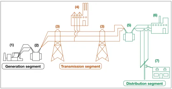
(20) 2.3. Electric power system’s structure Electric power systems are complex interconnected systems that are divided. in three distinct segments: generation, transmission and distribution; a simple network presented in Figure 2.2 illustrates this segmentation, present in this study. Currently, the development of new technologies is making power systems more complex by evolving to the smart grid concept. The electricity generation is carried out by power plants (1) that may use a wide range of resources (e.g. solar irradiance, water, oil, wind and coal) to produce energy with different technologies. This is done at a medium voltage and connected to a local substation (2), which constitutes a node of the network. The transmission segment starts at the substation (2) where voltage levels are increased in order to diminish losses, while it is being transported in transmission lines supported by towers (3) to another substation (5) in a different location where it is transformed to a medium or low voltage. The distribution segment starts at the substations (5), where it may be transformed to a low voltage to supply residential consumers (7) or may be kept at medium voltage to supply industrial consumers (4,6), which depending on the size could also be connected directly to the transmission segment (4). (4) (6) (3). (1). (3). (5). (2). (7) Generation segment. Transmission segment. Distribution segment. Figure 2.2. Electric power system’s structure (adapted from (S. Blume, 2007)). 19.

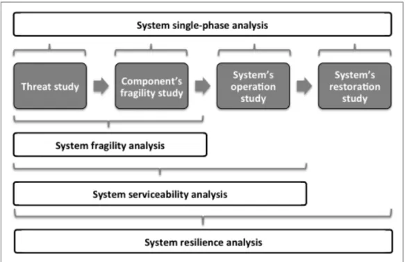
(21) The main components considered in the diagram and in this study are power plants, towers, transmission lines, substations and consumers (or loads). Power plants are composed of generation units, which are characterized by a number of technical parameters, such as their installed capacity, net (minus own consumption) active/reactive maximum/minimum generation, start-up times, variable costs, among others. Towers are vital components that support overhead power conductors, which are able to transport electricity constrained to their thermal capacity. Substations are facilities that are able to change the voltage from one level to another (with transformers), regulate the voltage, convert AC to DC and vice versa if required and is where safety/protection devices are installed, such as disconnect switches, circuit breakers, lightning arresters, etc. Loads are usually classified in industrial, commercial and residential consumers and represent the demand of the system.. 2.4. Types of risk analyses Various system evaluations may be performed depending in what is. included. As it is shown in Figure 2.3, in this work, a classification of four types of system analyses is proposed depending in what studies are included: a) Single-phase analysis: Commonly, because of the complexity of the problem, researchers have gone deep into the understanding of the threat (e.g. (V. Kaistrenko, 2014)), the development of fragility studies of components (e.g. (M. Sadeghi, M. Hosseini and N. Pakdel Lahiji, 2012)), models and tools to understand the operation of electric power systems (e.g. (F. Noakes and A. Arismundandar, 1963)) and models to manage and optimize system’s restoration (e.g. (N. Xu, et al., 2007)). These stages and their complexities are explained in more detail in Chapter 4. Even though these approaches might be useful, an. 20.

(22) integral point of view can result in a better understanding of the whole problem. b) System fragility analysis: Some authors have integrated the threat analysis and the system topology. This fragility analysis enables to understand the capacity post disaster of the system after a disastrous event by identifying which are the components that will commonly fail and those that may continue working (e.g. (H. Yang, et al., 2013)). c) System serviceability analysis: Research groups have integrated in a single study the threat study, the system topology and the system operation. When this is carried out, it may be considered as a vulnerability analysis. This permits to know the actual capacity of the system to supply the demand over a time frame (e.g. (J. Buritica, et al., 2012)). d) System resilience analysis: In the past few years, a number of authors have started to integrate the threat characterization, the system topology, the system operation and also the system restoration. This analysis is the most complete study and the approach taken in the present research (e.g. (M. Panteli and P. Mancarella, 2015; K. Pitilakis, et al., 2014; M. Ouyang and L. Dueñas-Osorio, 2014; M. Shinozuka, et al., 2007)).. 21.

(23) Figure 2.3. Types of system risk analyses (own elaboration).. 22.

(24) 3.. STATE OF THE ART AND CONTRIBUTIONS OF THIS THESIS Electrical power systems have been designed and operated to be reliable against. abnormal but foreseeable contingencies. The concept of reliability3, defined as the ability to supply adequate electric service on a nearly continuous basis, with very few interruptions over an extended time period (R. Billinton and W. Li, 1994), has been extensively applied in the electric sector. However, dealing with unexpected and less frequent severe situations remains a challenge. Resilience is an emerging concept and, as such, it has not yet been adequately explored in spite of its growing interest, particularly in power systems where there are almost no publications on the matter in IEEE periodicals (M. Panteli and P. Mancarella, 2015; H. Rudnick, 2011). This chapter aims at explaining different perspectives researchers from the power systems community have taken to analyse this problem. Then different methodological advances in the topic are presented and finally the contributions of this thesis are listed.. 3.1. Different perspectives for the resilience concept In 2014, the third number of the periodical IEEE Power and Energy. Magazine covered the resilience concept with the title “Surviving with resiliency“. The same year, CIGRE released the report “Disaster recovery within a CIGRE Strategic framework: network, resilience, trends and areas of future work”. This reflects the fact that resilience has become a major topic in the area. However, there is no consensus on how to treat the concept. Given the complexity of the problem and the system, it is understandable that different perspectives are taken. For example, within the mentioned IEEE PES Magazine issue, Article (G. Strbac, et al., 2015) is centred in how microgrids can enhance the resilience of the European megagrid. Here resilience is treated in a 3. Internationally, its main features are adequacy and security (R. Billinton and W. Li, 1994). In the Chilean technic normative quality of service is included as a third feature (CNE-Chile, 2015).. 23.

(25) dynamic time frame, where microgrids can help specifically in the islanding and restoration procedures. Article (C. Marnay, et al., 2015) focuses on the same issue and methodology, giving as example the microgrids developed in Japan. Article (M. Shahidehpour, et al., 2015) discusses how does an integrated lightning system in a smart city improve resilience by strengthening the mesh and adding redundancy. Two more articles, describe projects where different strategies are being used, such as hardening the system components, the deployment of microgrids as well as distributed and renewable generation devices and the automation of the system. With the exception of Article (M. Panteli and P. Mancarella, 2015), none of the above articles have developed an analysis of the system throughout the disaster in all of its stages. As (C.-C. Liu, 2015) suggests “a standardized definition of resiliency is needed to develop the requirements and procedures for (..) system planning and operation”.. 3.2. Methodological advances of resilience assessment and adaptation in electric power systems There are a few works related to power systems that take as base the curve in. Figure 2.1 and have a system perspective. Nevertheless, studies published in other fields are briefly described below. For instance, in (K. Pitilakis, et al., 2014), a joint effort of European universities analyses the impact of earthquakes on various cities and different critical infrastructures, including the power systems of Sicily. This study included the use of fragility curves and an object-oriented programme to assess the pre- and post-disaster performance of the network. In (M. Panteli and P. Mancarella, 2015), the impact of windstorms is analysed using wind fragility curves, running DC optimal power flows on the IEEE-6 bus reliability test system and comparing different adaptation cases.. 24.

(26) The resilience of the electric system of Harris County, Texas, US, is evaluated in (M. Ouyang and L. Dueñas-Osorio, 2014) by running four models: hurricane hazard model, components fragility model, power system response model and restoration model. The results are classified in technical, organizational and social dimensions of resilience. In (Shinozuka, et al., 2007), micro-components of the transmission network under seismic stress are modelled to assess the resilience of the power system in Los Angeles, US. The vulnerability is also modelled, with fragility curves and risk curves developed as results. Another notable effort, that has involved software developments, is Hazus, from the Federal Emergency Management Agency (FEMA) (2015). This platform has developed various fragility curves with damage states for many systems, some of them used in this research. Even though the recent work on the topic has been a huge step towards understanding and measuring resilience, further research in this area remains a concerning issue given the consequences of these and other catastrophic threats to different systems around the world.. 3.3. Contributions of the present work In the present work, the novel contributions are listed below: An integral analysis with a system perspective covering the whole. disaster process is carried out to confront the problem of natural disasters and electric power systems. It is common to find in literature that researchers studying disaster management and power systems choose single-phase approaches where the intention is limited to individual elements at risk. A novel multi-phase resilience assessment and adaptation framework is formalized by identifying the best practices in recent international literature.. 25.

(27) Three different natural hazards and two electric power systems are modelled to apply the resilience framework presented. Therefore, comparisons are possible. In all publications found about the topic, only a single hazard and system is modelled. The test systems are representative of national grids with focus on the generation and transmission system, where potential impacts are wider, but with fewer details. In most publications the test system is focused on the distribution level, losing a national perspective and being unable to apply national strategies. Multi-disciplinary work was carried out, with people from public and private organizations and from different countries. Due to the complexity of resilience studies, different fields have to be involved to be able to cover the whole process.. 26.

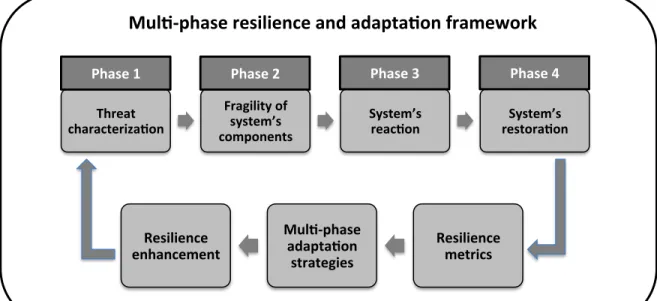
(28) 4.. MULTI-PHASE. RESILIENCE. ASSESSMENT. AND. ADAPTATION FRAMEWORK In this chapter, the resilience and adaptation framework presented in Figure 4.1, and given in detail in Appendix B, is proposed for evaluating the impact of natural disasters on the resilience of electric power systems4 and the effect of possible adaptation strategies. This framework is presented in detail next.. Mul$%phase+resilience+and+adapta$on+framework+ Phase+1+. Phase+2+. Phase+3+. Phase+4+. Threat+ characteriza$on+. Fragility+of+ system’s+ components+. System’s+ reac$on+. System’s+ restora$on+. Resilience+ enhancement+. Mul$%phase+ adapta$on+ strategies+. Resilience+ metrics+. Figure 4.1. The multi-phase resilience and adaptation framework (own elaboration).. 4.1. Multi-phase resilience assessment The resilience assessment consists of four phases: threat characterization,. fragility of the system’s components, the reaction of the system and finally its restoration.. 4. Even though the resilience framework proposed can be extended to study any threat and any critical infrastructure, the study focuses in power systems so the phases do not incorporate aspects that may be of importance to other systems.. 27.

(29) 4.1.1 Phase one: threat characterization The objective of this phase is to model the magnitude, probability of occurrence and spatiotemporal profile of a hazard. To this end, the causes, physical aspects and consequences of the threat must be understood. Two approaches can be taken, one is to build deterministic scenarios, where a historic event is modelled, and the other one is to build probabilistic scenarios, where potential future scenarios are projected. For deterministic modelling, depending on the natural hazard under investigation, different tools can be used. For extreme weather events, generally the weather database needed may be acquired through Climate Models (CM), which can model the threat with a certain geographic and time resolution, or using real measurements with time a geographic features from weather stations. In the case of seismic and tsunami hazards seismographs and sea-level measurements database should be used. For probabilistic scenarios, different projection methods can be used. The selected method has to be suitable to be applied to the specific event (e.g. earthquakes, tsunamis, floods, etc.) and be able to make an estimate of anticipated forces, possibly much greater than have ever been observed, using historical or model-generated data. For the case of data generated by CM, parametric studies are useful, where the parameters are modified by a certain factor (usually taking in consideration real extreme measurements or expert knowledge). For the case of instrumentally measured data, a first option is Power Law, which has modelled numerous natural phenomena, such as the Gutenberg-Richter number-size distribution of earthquake magnitude and other probabilistic predictions of data behaviour (S. Burroughs and S. Tebbens, 2001). Specifically for earthquakes, as developed by (B. Gutenberg and C. Richter, 1994) and explained in (A. Poulos,. 28.

(30) 2014), each seismic source has an annual amount of earthquakes that exceeds a given magnitude, which is represented by Equation 4.1.. 𝑙𝑜𝑔!" 𝜆! 𝑚. = 𝑎 − 𝑏𝑚. (4.1). Where 𝜆! 𝑚 is the mean annual frequency of the seismic events that exceeds magnitude m, and coefficients a and b are estimated by regressions. Given lower and upped bound magnitudes Mmin and Mmax, respectively, the cumulative distribution function (CDF) of the magnitude of an earthquake 𝑀!"# ≤ 𝑀 ≤ 𝑀!"# is presented in Equation 4.2 and its probability density function is presented in Equation 4.3.. 𝐹! 𝑚 = 𝑃 𝑀 ≤ 𝑚 = . 𝑓! 𝑚 = 𝑃 𝑀 = 𝑚 = . !!!"!!(!!!!"# ) !!!". !!(!!"# !!!"# ). !∗!" !" ∗!"!!(!!!!"# ) !!!". !!(!!"# !!!"# ). (4.2). (4.3). A second option for instrumentally measured data, is Extreme Value Theory (EVT) (S. Coles, 2001), which is based on the distribution of the maximums (or minimums) by defining a return period T (e.g. 100-years) and estimating its return value X(T) (e.g. 60 mm). This would mean that an event of X(T) is estimated to happen every T years. EVT has two main approaches: Block Maxima Approach (BMA) and Peaks Over Threshold (POT). Both approaches have the aim of estimating X(T) for rare extreme events. In the case of BMA, this is done by a parametric modelling of maximums (or minimums) taken from large blocks of independent data. In the case of POT, this is done by a parametric modelling of independent exceedances above a large (or low) threshold. Both approaches then. 29.

(31) use the Generalized Extreme Value (GEV) distribution (A. Jenkinson, 1955; J. Hosking, J. Wallis and E. Wood, 1985). GEV has the flexibility of combining the three types of extreme distributions, namely Type I-Gumbel, Type II-Fréchet and Type III-Weibull. GEV’s cumulative distribution function (CDF) is as follows:. 𝐹 𝑥; 𝜓, 𝛽, 𝜉 = 𝑒. !(!!! . ! !!! !! ) !. , 𝑓𝑜𝑟 1 +. !(!!!) !. >0. (4.4). In Equation 4.4, 𝜓 (location), 𝛽 (scale) and 𝜉 (shape) are the three main parameters of GEV. The particular cases of 𝜉 = 0, 𝜉 > 0 and 𝜉 < 0 are respectively equivalent to the distributions Type I, whose tails decrease exponentially; Type II, whose tails decrease as a polynomial and Type III, whose tails are finite. When the parameters are estimated to fit the dataset, a projection diagram can be drawn to visualize the return periods and return values (E. Gumbel, 1958).. 4.1.2 Phase two: fragility of system’s components The aim of this phase is to determine the damage level of each component of the system. To do this, the following three steps are considered: i.. identify the vulnerable components. ii.. fragility modelling of the components. iii.. assign damage states In the first step, the components identified are those that are vulnerable to. the threat that could possibly have a high impact on the network resilience. Also, the type of component must be selected. In electric power systems, components can be classified in macro or micro components (K. Pitilakis, et al., 2014). For example, high/medium/low voltage substations/power plants, distributions circuits, transmission towers and lines can be classified as macro components. Circuit breakers, transformers, lightning arresters, switches and all those elements that 30.

(32) describe the internal logic of macro components are micro components. The use of one or another depends on the objectives of the resilience study being undertaken. Some studies also propose modelling people and communities from a physiologic perspective (M. Bruneau, et al., 2003; K. Bergstrand, et al., 2014). The second step corresponds to modelling the fragility of the components to the natural threats. The concept of Fragility Curves has its origins as a structural reliability concept (JCOSS, 1981; F. Casciati and L. Faravelli, 1991), and is a useful tool for a stand-alone analysis of each component. A fragility curve, as shown in Figure 4.2, expresses the probability of failure of a component conditioned on the impact of the hazard. In practice, these failure probabilities are compared with a uniformly distributed random number r~U(0,1). If the failure probability of the component is larger than r, then the component fails.. Figure 4.2. Generic fragility curve: probability of failure (%) vs threat parameter (own elaboration). It is important to note that a “failure“ of the component does not necessarily imply a complete collapse of the component (i.e. removal from service). For example, after a seismic event a power plant that is composed of more than one generation unit might have just a portion of the units out of service, meaning that the power plant will be able to work at a degraded maximum generation capacity.. 31.

(33) At the same time, other components such as transmission lines have a binary damage state: tripped or non-tripped. Thus, as a third step, the damage state of the components must be addressed. In order to do this, two approaches can be used as shown in Figure 4.3, where (a) uses different fragility curves for different damage levels (as used by (FEMA, 2015)) and (b) relates the damage level to the zone of the fragility curve defined by percentiles (as used in Chapter 5). Particularly for electric power systems, even though, most frequent faults happen at a distribution level, less common but with a higher impact occur at a transmission and generation level. Because of this, and to be able to have a nationwide perspective of resilience this research focuses on the generation and transmission level components.. Figure 4.3 (a). Different fragility curves to assign damage states. (b). Different zones in the fragility curve to assign damage states. (Own elaboration). 4.1.3 Phase three: system’s reaction The objective of the third phase is to evaluate the performance of the critical infrastructure when it is exposed to the extreme event. In electrical power systems, to do this, numerous evaluation tools have been developed over the last decades; such as the CASCADE model, which studies the cascading mechanism of a blackout (I. Dobson, A. Carreras and D. Newman, 2003); the ORNL-PSERC-. 32.

(34) Alaska (OPA) model, which is based on a DC optimal power flow and it is built upon Self-Organized Criticality (B. Carreas, V. Lynch, I. Dobson and D. Newman, 2002; I. Dobson, A. Carreras and D. Newman, 2001); the Hidden Failure model, which is based on approximated DC power flow and standard linear programming optimization of generation redispatch to represent hidden failures of the protection system (J. Chen, J. Thorp and I. Dobson, 2005); and the Manchester model, which is built upon AC power flow, uses load shedding and a power flow solution to determine the power system operation (M. Rios, et al., 2002; D. Kirschen, et al., 2003, D. Kirschen, et al., 2004). When modelling the impact of extreme natural events, it is important to take into account the diverse impact of the weather front or geographic profile moving across the system, which is both spatial- and temporal-dependent. The resilience model used in this phase should thus be capable of capturing the spatiotemporal stochastic impact of the natural disaster on the resilience of power systems. It has to consider the flexibility of the system given by the installed technology and possible international interconnections. It should also be capable of providing a component and area criticality index, which will enable the resilience enhancement of the most vulnerable components. Furthermore, following the disaster, it is very likely that the system will be divided into multiple islands, which should be incorporated in the impact assessment model. 4.1.4 Phase four: system’s restoration The response to the disaster and the restoration times following the disaster are strongly related to the following three aspects: i.. damage caused. ii.. amount of human and material resources available. iii.. accessibility of the affected area. The restoration process can only be undertaken under the condition that both. repair-teams and spare parts are available. The fast restoration and recovery of. 33.

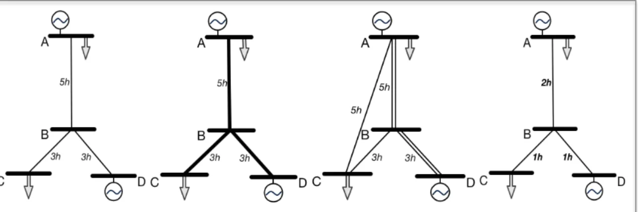
(35) critical infrastructure is a crucial feature of resilience (as discussed in Chapter 2). Therefore, proper and effective emergency and restoration strategies should be in place to restore the system to its pre-disaster state as fast as possible. 4.2. Multi-phase adaptation strategies The probability of extreme weather events is relatively low, but their impact. is so high that is vitally important to enhance the resilience of critical infrastructures. Particularly, for electric power systems, this can be achieved through a wide range of short- and long-term measures. Short-term measures are discussed in detail in (M. Panteli and P. Mancarella, 2015a; M. Panteli and P. Mancarella, 2015b). Long-term measures can be grouped in strategic adaptation cases that improve specific phases of the resilience of the system. Namely, the cases are: (i) Normal, which is the basic network; (ii) Robust, that improves the resistance of the system; (iii) Redundant, which includes backup installations or spare capacity enabling the diversion of the power flows to alternative paths of the network; and (iv) Responsive, that enables a faster response from the disruptive events. It can thus be seen that these adaptation case studies can improve, respectively, the 2nd, 3rd and 4th phases of the resilience framework.. Figure 4.4 (a). Normal case. (b). Robust case. (c). Redundant case. (d). Responsive case. (Own elaboration. Numbers indicate mean time to repair).. 34.

(36) Explicative diagrams of the adaptation cases are presented in Figure 4.4 (based on the examples in (C. Pickering, S. Dunn and S. Wilkinson, 2013), where (a) represents the normal network, which consists of four nodes and three links with their mean times to repair, (b) represents the robust case, having more resistant links that can be interpreted as a shift of the fragility curve. (c) shows the redundant case including alternative paths and (d) is the responsive case, where the mean times to repair are decreased. 4.3. Resilience metrics Depending on the aim of the resilience study, the performance of electric. power systems can be measured using numerous different metrics. Two measurements that are able to describe the impact of the extreme event within a time frame are the Expected Energy Not Supplied (EENS) and the Energy Index of Unreliability (EIU) (R. Billinton and W. Li, 1994, R. Allan and R. Billinton, 2000). The first, shown in Equation 4.5, indicates how much service (energy) was not provided during the studied time period as an absolute number (MWh or GWh). The second, shown in Equation 4.6, is directly related to EENS, which is normalized using the total energy demand in the studied time frame (%). In the following equations, 𝐸! is the energy not supplied with a probability 𝑝! of occurrence of scenario k during the time frame of the study. E represents the energy demand in the whole study period. !!!. 𝐸𝐸𝑁𝑆 𝐺𝑊ℎ = . 𝐸! ∗ 𝑝! . (4.5). !!!. 𝐸𝐼𝑈 % = . 𝐸𝐸𝑁𝑆 ∗ 100% 𝐸. 35. (4.6).

(37) 4.4. Resilience modelling In the previous sections of this chapter, the framework concepts have been. explained. In Figure 4.5, a flow chart of the resilience framework is displayed. The model is based on Sequential Monte Carlo Simulations, where every grey box represents one scenario and within every scenario an hourly sequential simulation is run. It has to be noted that the applications in following chapters may differ from the present flow chart.. Read inputs Load system case (lines, buses, generators). Set Nhours, Initial component damage states, initial operation state of units. Set ENS to 0.. scenario = s. Hazard scenario Apply deterministic or probabilistic method for event. hour = 1…Nhours Initialization of parameters Hourly power and reactive demand per bus. Hazard hourly scenario Hourly intensity measure of event in every component site (e.g. wind speed, peak ground acceleration, etc).. Impact on components Run fragility curve analyses for every component. Assign damage states.. Restoration of components For all components: Is component damaged? yes no. Subject to human and resources availability, event intensity and damage state assign time to repair.. Is time to repair < hour yes Component damage state = normal.. System operation Set operation state of the system (emergency and normal). Island handling. With online components run OPF of this hour.. Resilience metrics ENS = ENS + Energy not supplied this hour.. Figure 4.5. Resilience modelling flow chart (own elaboration). 36.

(38) 5.. APPLICATION TO WINDSTORMS AND FLOODS IN GREAT BRITAIN In the present chapter, the multi-phase resilience framework previously presented. is illustrated by assessing the impact of potential future scenarios of windstorms and floods on a reduced version of the Great Britain’s electric power system as it is explained hereafter.. 5.1. Influence of extreme weather and climate change in Great Britain’s power system In this Section, extreme weather events are described along with the. influence of climate change and possible future scenario hazards.. 5.1.1 Extreme weather events A disruptive weather event can be classified into small, moderate, serious, major and extreme based on the number of customers disconnected, the duration and frequency (W. Associates, 2011). For example, in the USA, extreme weatherrelated events account approximately for 80% of the large-scale power outages from 2003 to 2012 (A. Kenward and U. Raja, 2014), with the annual impact ranging from $20 to $55 billion (R. Campbell, 2012). Great Britain, in particular, is significantly affected by weather-related power outages. In (L. McColl, et al., 2012), it is reported that only from April 2008 to March 2009, 211 faults occurred on the transmission network in England and Wales and other 44 in Scotland, of which 23% and 95% were caused by weather, respectively. These weather-related faults can be categorized in one of eight causes: wind and gale; snow; sleet and blizzard; lightnings; ice; freezing fog and frost; heat waves; flooding and rain (L. McColl, et al., 2012; K. Murray and K. Bell, 2014). For example, several transmission substations and power stations are. 37.

(39) at high risk of flooding, while high winds can cause transmission lines and towers to collapse. Also, in 2007, Great Britain suffered the wettest summer in its history. This produced extreme rainfall compressed into short periods of time that caused a series of destructive floods catalogued as the country’s “largest peacetime emergency since World War II“ (M. Pitt, 2008). Moreover, a few years later in 2014, an even more extreme weather-year took place. As described by the National Meteorological Office (MET), this was the wettest, 5th warmest and probably most disastrous winter in the UK (MET Office, 2014). Consequently, the Climate Change act of 2008 required the UK electricity industry to report on adaptation measures to deal with the effects of weather and the effect of climate change (United Kingdom Parliament, 2008). This motivates to analyse particularly windstorms and floods in this research.. 5.1.2 Climate change and future hazard scenarios In 1992, the United Nations Framework Convention on Climate Change (UNFCCC) was created with the objective to “stabilize greenhouse gas concentrations in the atmosphere at a level that would prevent dangerous anthropogenic interface with the climate system“ (R. Pachauri and L. Meyer, 2014). To achieve this, the Intergovernmental Panel on Climate Change (IPCC) supports UNFCCC producing reports of the scientific, technical and socioeconomic aspects of global warming with its potential impacts and options for adaptation and mitigation. Until today, a series of five comprehensive reports have been published. The latest one, in 2014, stated that now, the IPCC, is “95% certain that humans are the main cause of current global warming“ and that “climate change will amplify existing risks and create new risks for natural and human systems“ (R. Pachauri and L. Meyer, 2014). Even though, mitigation of Greenhouse Gases (GHG) is crucial to constrain climate change, adaptation of infrastructure becomes essential, before mitigation measures can have any effect. 38.

(40) (N. Stern, 2006). In consequence, possible future changes in natural hazards must be analysed. According to the IPCC, climate change projections may vary from region to region, but generally it is likely that wet and dry extremes are going to become more severe (R. Pachauri and L. Meyer, 2014). In Great Britain, particularly for the variables studied here, reports indicate that while wind has a high uncertainty on how it will change (L. McColl, et al., 2012), flood risk will escalate because of the potential increase of rainfall volume and intensity (E. Evans, et al., 2008). Unfortunately, quantitative studies disagree on how will they scale up (L. McColl, et al., 2012). 5.2. The Great Britain’s simplified electric power system The Great Britain network used in this study is a simplification5 of the real. one at the end of 2010 (M. Belivanis and K. Bell, 2011). As it is shown in Figure 5.1 (a), the grid consists of 29 nodes, 98 overhead transmission lines in double circuit configuration and one single circuit transmission line between nodes 2 and 3, and 65 generators (with 81.5 GW of installed capacity) which are located at 24 nodes and include several technologies, such as wind, nuclear and CCGT. Nodes Transmission route – double circuit OHL Transmission route – single circuit OHL. 1. Weather Region. 2. 1. 2. 1 3. 3. 4. 4 5. 2. 7. 6. 5. 8. 7. 6. 8 10. 9. 10. 9. 4. 3. 15. 11 12. 13. 16. 14. 12. 17. 22. 29. 24 28. 13. 16. 14 17. 19. 19. 18 23. 15. 11. 25. 18. 20. 21. 22 23. 26. 5. 27. 29. 24 28. 25. 20. 21 26. 27 6. 5. The components are not real; they represent a group of real components while trying to replicate the real AC power flows and operation of the actual system.. 39.

(41) Figure 5.1 (a). Great Britain’s simplified system. (b). Weather regionalization of the system. (Own elaboration with M. Panteli). Interconnections with external subsystems, i.e., France, the Netherlands and Northern Ireland are included. The demand, plotted in Figure 5.2, represents the winter peak week in 2010.. 50000. 50000. Active power 45000. Reactive power. 40000. 40000. 35000. 35000. 30000. 30000. 25000. 25000. 20000. 20000. 15000. 15000. 10000. 10000. 5000. 5000. 0. Reactive power demand [MVAr]. Active power demand [MW]. 45000. 0 1. 8. 15. 22. 29. 36. 43. 50. 57. 64. 71. 78. 85. 92. 99 106 113 120 127 134 141 148 155 162. Time [hour]. Figure 5.2. Winter peak demand week in Great Britain (Own elaboration).. 5.3. Resilience assessment The resilience of the test network is evaluated against windstorms and. floods, which constitute severe threats to the Great Britain system.. 5.3.1 Phase one: windstorms and floods characterization As explained in detail in Section 4.1.1, the threat characterization phase aims at defining the event’s probability of occurrence, magnitude and spatio-temporal profile. Therefore, in order to account for the spatial feature of the weather events, the “big island” is divided into 6 weather regions, as shown in Figure 5.1 (b).. 40.

(42) Weather conditions are assumed to be homogeneous within each region, so the fragility of each component is conditioned to the same stress across each weather region. Potential future scenarios were modelled as explained hereafter. For the windstorms modelling, the main characteristic is the geographic mapping of the location and magnitude of wind speed. Therefore, hourly mean wind data for 33 years (1979-2011) was obtained using MERRA re-analysis (NASA, 2015). On the other hand, floods are more complex and affected by many factors, such as the capacity of drainage system, saturated ground, high river levels and accumulated rainfall. But in general, especially river and groundwater floods are strongly related to rainfall. For example, in (P. Guhathakurta, et al., 2011) flood is linked directly to accumulated rainfall. The hourly rainfall data for the same years, i.e., 1979-2011, was obtained from more than 17000 rain gauge stations all over Great Britain in that time frame, which was provided by the MET Office, UK (MET Office, 2006). This analysis altogether provides the temporal characterization of the threats: 33 years of wind and rainfall profiles with hourly resolution. In order to deal with the uncertainty associated with the future weather conditions as a direct impact of climate change, five scenarios have been developed for evaluating the impact of windstorms, floods and both hazards together. Given that wind speed was taken from a Climate Model, where the focus is on average measurements (with a maximum average of approximately 20 m/s), one suitable approach to use in order to model extreme winds that can damage the transmission components is to parametrically scale up the wind profiles. Therefore, the winds profiles of the 6 weather regions have been scaled up using a multiplication factor in the range [1,3] in steps of 0.5, resulting in five windstorms scenarios (meaning that x2 and x3 would represent approximately wind speeds of 40 m/s and 60 m/s, respectively). The wind profile is scaled up by the same factor. 41.

(43) in the whole network, so the impact affects the entire network instead of specific areas. For floods, given that the rainfall data was taken from real measurements, five levels were modelled by applying extreme value theory. Assuming the data is independent and identically distributed, the Block Maxima Approach (BMA) and the Generalized Extreme Value (GEV) distribution was used. Then the parameters of the GEV distribution were estimated to fit the dataset and a projection diagram was drawn for each region. An example of a projection diagram for Region 4 is shown in Figure 5.3.. Figure 5.3. Projection diagram for Region 4 - horizontal axis in logarithmic scale - (own elaboration). Thereafter, five return periods were chosen (i.e. 10-year, 33-year, 100-year, 150-year and 250-year), which provided five return values for the peak rainfall within one hour for every region. For example, for Region 4 the return values projected were: 17 mm, 32.9 mm, 59.7 mm, 74.1 mm and 97 mm, respectively (which is reasonable taking into account that the highest hourly rainfall recorded by Met Office was 92 mm in 1901 (MET Office UK, 2015). Then, rainfall scale parameters are calculated with Equation 5.1, where given a return period λ-year, the scale parameter, π γ, ρ, λ , for the year γ and region ρ is equal to the return. 42.

(44) value Τ (𝜆-year) [mm] divided by the peak rainfall value of the year γ in the region ρ, Ρ (γ, ρ) [mm]. 𝜋 𝛾, 𝜌, 𝜆 = . ! (!!!"#$) ! (!,!). , 𝑓𝑜𝑟 𝛾 ∈ [1979, . . ,2011]. (5.1). 5.3.2 Phase two: fragility of electrical components As detailed in Section 4.1.2, the component’s fragility phase should follow three steps: first identify the vulnerable components, then use a fragility curve approach and finally assign damage states. Therefore, in the Great Britain study case, the key vulnerable macro components shown in Table 5.1 were identified and modelled. Table 5.1. Threats analysed with their correspondent key vulnerable components identified (own elaboration). Threat Wind Storms Floods. Vulnerable components Transmission lines Substations. Transmission towers Power plants. Subsequently, the vulnerability of each identified component is analysed through fragility curves. Used lines and towers’ wind fragility curves are presented in Figure 5.4.(a) (M. Panteli and P. Mancarella, 2015). Likewise, in Figure 5.4.(b), the flood fragility curves used are shown. Floods are strongly related to the accumulated rainfall, which can be produced by an intense short event (less than three hours) or a prolonged event (less than ten hours). These imply that beginning with rainfalls of approximately 20 mm/hour for at least three hours, the risks of flooding exist (D. Houston, et al., 2011). To take into account the particularities of power stations and substations, when a flood occurs, a probabilistic assignation is done (i.e. 38% for power plants and 33% for substations) based on the report on the survey of electrical components at flood risk in (H. Wallingford, 2014). The accuracy of these curves can vary depending on the particularities of each. 43.

(45) component. Consequently the accuracy of the assessment can be improved in further works by improving the methods to generate the fragility curves.. Figure 5.4. (a) Lines and tower’s fragility curves (M. Panteli and P. Mancarella, 2015). (b) Floods by intense or prolonged rainfall fragility curves (own elaboration with data from (D. Houston, et al. 2011)).. Finally, following the failure of a component, the damage state has to be assigned. The approach in this study is to establish the damage through zones in the fragility curve as shown in Figure 4.3. (b). For example, power plants have four possible damage states: minor, moderate, extensive and complete. These states are determined by the percentiles 0-25th, 25th-50th, 50th-75th and 75th-100th, respectively. Lines, towers and substation’s potential damage are modelled with two states: operative and non-operative.. 5.3.3 Phase three: power system’s reaction As detailed in Section 4.1.3, the system’s operation phase consists in Sequential Monte Carlo Simulations with hourly OPF analyses. Also, in order to capture the spatiotemporal impact of the wind and rainfall fronts moving across the transmission network, a Sequential Monte Carlo-based time-series simulation model has been developed. This enables the representation of the weather and. 44.

(46) electrical events in a chronological order as they happen in reality at different locations of the test system. An hourly simulation step is used, which is considered sufficient for modelling weather events. However, any time resolution can be used if desired and provided that the relevant information is available, e.g., weather profile. Further, one winter week is used as a simulation period, where extreme wind and rainfall events are expected considering that severe weather events do not usually last longer in Great Britain. At every simulation step, the wind- and rainfall-affected failure probabilities of the electrical components obtained by the fragility curves are fed to the timeseries simulation model as explained in the previous phases. Following this approach, the real-time weather-adjusted operation state of each electrical component is obtained. An AC Optimal Power Flow (OPF) is used for assessing the performance of the test network at every simulation step, which helps determine if load shedding is required for stabilizing the system. For solving the power flows the Netwon method was used, and for the optimization problem Matlab Interior Point Solver (MIPS) was employed. Finally, the model is also capable of island handling.. 5.3.4 Phase four: power system’s restoration As explained in Section 4.1.4, three aspects should be taken into consideration for the components restoration: damage caused, human and material resources availability and the accessibility to the affected area. In this study, for simplicity reasons, the restoration curves are only related to the difficulties of the repair crew to enter the affected areas. The component restoration curves are defined by exponentially distributed curves with mean parameters as shown in Table 5.2. A Mean Time To Repair (MTTR) of 10 hrs and 50 hrs is assumed for lines and towers respectively, and 10 hrs and 30 hrs for power plants and substations respectively (referred to as MTTRbase). The weather intensity is. 45.

(47) classified here as follows: for windstorms, it can be Low (less than 20 m/s), Moderate (between 20 m/s and 40 m/s) or High (more than 40 m/s), while for floods it can be Low (less than 138 mm for intense accumulated rainfall or 280 mm for prolonged accumulated rainfall or High (more than 138 mm for intense accumulated rainfall or 280 mm for prolonged accumulated rainfall). As weather intensity increases, the repair crews need more time to enter the affected area and restore the damaged components, which is modelled here as a random increase in MTTRbase as can be seen in Table 5.2. Table 5.2. Mean times to repair (hours) for different weather intensities (own elaboration). Threat Windstorms Floods. 5.4. Component Lines Towers Power Plants Substations. MTTR for different weather intensities (Wind speed (m/s) / Accumulated rainfall (mm)) Low Moderate High MTTRbase MTTRbase MTTRbase MTTRbase. MTTRbase×rand[2,4] MTTRbase×rand[2,4] -----. MTTRbase×rand[5,7] MTTRbase×rand[5,7] MTTRbase×2 MTTRbase×2. Resilience adaptation In this study, the adaptation strategies discussed in Section 4.2 are applied to. the critical transmission route shown in Figure 5.5 from North to South Great Britain. Following extensive resilience studies (mainly focusing on the maximum power flows on the transmission lines), this corridor was identified as one of the critical transmission routes for preserving the resilience of the entire power system. Particularly, for the normal case, the basic network was used with no resilience enhancement. For the robust strategy case, the fragility curves of the components (see Figure 5.4) in the critical path were shifted to the right a 15% of the 50th percentile of the curve. For the redundant strategy case, identical parallel lines have been added to the critical transmission path. Finally, for the responsive. 46.