The Next Generation Virgo Cluster Survey (NGVS) XXXI The Kinematics of Intracluster Globular Clusters in the Core of the Virgo Cluster

Texto completo

(1)The Astrophysical Journal, 864:36 (23pp), 2018 September 1. https://doi.org/10.3847/1538-4357/aad3d2. © 2018. The American Astronomical Society. All rights reserved.. The Next Generation Virgo Cluster Survey (NGVS). XXXI. The Kinematics of Intracluster Globular Clusters in the Core of the Virgo Cluster Alessia Longobardi1 , Eric W. Peng1,2 , Patrick Côté3 , J. Christopher Mihos4 , Laura Ferrarese3 , Thomas H. Puzia5 Ariane Lançon6 , Hong-Xin Zhang5,7 , Roberto P. Muñoz5, John P. Blakeslee8,9 , Puragra Guhathakurta10 , Patrick R. Durrell11 , Rúben Sánchez-Janssen12 , Elisa Toloba13, Andrés Jordán5,14 , Susana Eyheramendy14,15, Jean-Charles Cuillandre16, Stephen D. J. Gwyn8, Alessandro Boselli17 , Pierre-Alain Duc6 , Chengze Liu18 , Karla Alamo-Martínez5 , Mathieu Powalka6 , and Sungsoon Lim2. ,. 1. Kavli Institute for Astronomy and Astrophysics, Peking University, Beijing 100871, People’s Republic of China; alongobardi@pku.du.cn 2 Department of Astronomy, Peking University, Beijing 100871, People’s Republic of China; peng@pku.edu.cn 3 NRC Herzberg Astronomy and Astrophysics, National Research Council, 5071 West Saanich Road, Victoria, BC V9E 2E7, Canada 4 Department of Astronomy, Case Western Reserve University, Cleveland, OH 41106, USA 5 Institute of Astrophysics, Pontificia Universidad Católica de Chile, Av. Vicuña Mackenna 4860, 7820436 Macul, Santiago, Chile 6 Observatoire Astronomique de Strasbourg, Université de Strasbourg, CNRS, UMR 7550, 11 rue de l’Université, F-67000 Strasbourg, France 7 CAS Key Laboratory for Research in Galaxies and Cosmology, Department of Astronomy, University of Science and Technology of China, Hefei 230026, People’s Republic of China 8 NRC Herzberg Astronomy and Astrophysics, 5071 West Saanich Road, Victoria, BC V9E 2E7, Canada 9 Gemini Observatory, Casilla 603, La Serena 1700000, Chile 10 UCO/Lick Observatory, University of California, Santa Cruz, 1156 High Street, Santa Cruz, CA 95064, USA 11 Department of Physics and Astronomy, Youngstown State University, Youngstown, OH 44555, USA 12 UK Astronomy Technology Centre, Royal Observatory Edinburgh, Blackford Hill, Edinburgh, EH9 3HJ, UK 13 Department of Physics, University of the Pacific, 3601 Pacific Avenue, Stockton, CA 95211, USA 14 Millennium Institute of Astrophysics, Av. Vicuña Mackenna 4860, 7820436 Macul, Santiago, Chile 15 Department of Statistics, Faculty of Mathematics Pontificia Universidad Católica de Chile, Av. Vicuña Mackenna 4860, 7820436 Macul, Santiago, Chile 16 CEA/IRFU/SAp, Laboratoire AIM Paris-Saclay, CNRS/INSU, Université Paris Diderot, Observatoire de Paris, PSL Research University, F-91191 Gif-sur-Yvette Cedex, France 17 Aix Marseille Université, CNRS, LAM (Laboratoire d’Astrophysique de Marseille) UMR 7326, F-13388 Marseille, France 18 Department of Astronomy, Shanghai Key Laboratory for Particle Physics and Cosmology, Shanghai Jiao Tong University, Shanghai 200240, People’s Republic of China Received 2018 March 23; revised 2018 July 6; accepted 2018 July 14; published 2018 August 29. Abstract Intracluster (IC) populations are expected to be a natural result of the hierarchical assembly of clusters, yet their low space densities make them difficult to detect and study. We present the first definitive kinematic detection of an IC population of globular clusters (GCs) in the Virgo cluster, around the central galaxy M87. This study focuses on the Virgo core, for which the combination of Next Generation Virgo Cluster Survey photometry and follow-up spectroscopy allows us to reject foreground star contamination and explore GC kinematics over the full Virgo dynamical range. The GC kinematics changes gradually with galactocentric distance, decreasing in mean velocity and increasing in velocity dispersion, eventually becoming indistinguishable from the kinematics of Virgo dwarf galaxies at R>320 kpc. By kinematically tagging M87 halo and intracluster GCs, we find that (1) the M87 halo has a smaller fraction (52±3%) of blue clusters with respect to the IC counterpart (77±10%), (2) the (g′−r′)0 versus (i′−z′)0 color–color diagrams reveal a galaxy population that is redder than the IC population, which may be due to a different composition in chemical abundance and progenitor mass, and (3) the ICGC distribution is shallower and more extended than the M87 GCs, yet still centrally concentrated. The ICGC specific frequency, SN,ICL=10.2±4.8, is consistent with what is observed for the population of quenched, low-mass galaxies within 1 Mpc from the cluster’s center. The IC population at Virgo’s center is thus consistent with being an accreted component from low-mass galaxies tidally stripped or disrupted through interactions, with a total mass of MICL,tot = 10.8  0.1 ´ 1011 M. Key words: galaxies: clusters: individual (Virgo) – galaxies: individual (M87) – galaxies: kinematics and dynamics – galaxies: star clusters: general – globular clusters: general stellar properties. In dense environments, accretion is even more dramatic, such that close to the dynamical center of clusters, central galaxies are expected to have accreted a majority of their stars (Laporte et al. 2013; Cooper et al. 2015). In galaxy clusters, a fraction of their baryonic content is represented by the intracluster light (ICL, or “diffuse light”), a component that is gravitationally unbound to cluster galaxies but bound to the cluster potential (e.g., Murante et al. 2004; Rudick et al. 2006; Dolag et al. 2010; Puchwein et al. 2010; Contini et al. 2014). Galaxy interactions and tidal interactions between galaxies and the cluster potential are both believed to. 1. Introduction Mergers are believed to play a dominant role in the assembly of massive galaxies (De Lucia & Blaizot 2007). A two-phase formation scenario (Naab et al. 2009) predicts that in a first dissipative phase (high redshift, z2) stars form quickly and build the compact innermost regions of massive galaxies (with stars rich in α elements; Thomas et al. 2005); later, minor mergers dominate the mass assembly in the outermost regions (Oser et al. 2010), and the accretion of metal-poor stars from smaller stellar systems results in the variation of the galaxy 1.

(2) The Astrophysical Journal, 864:36 (23pp), 2018 September 1. Longobardi et al.. Forte 2001; Kundu & Whitmore 2001; Larsen et al. 2001; Puzia et al. 2005a, 2005b; Peng et al. 2006; Leaman et al. 2013; Tonini 2013; Harris et al. 2017). The most popular division uses optical colors to identify a red (metal-rich) and a blue (metal-poor) population of GCs, although the existence of an additional, intermediate, population of GCs has been claimed (Peng et al. 2009; Strader et al. 2011; Agnello et al. 2014). To these different classes correspond different observed properties, so red and blue GCs are measured to have different kinematics and spatial distribution (Zepf et al. 2000; Côté et al. 2001, 2003; Schroder et al. 2002; Perrett et al. 2003; Peng et al. 2004; Schuberth et al. 2010; Strader et al. 2011; Coccato et al. 2013; Agnello et al. 2014; Zhang et al. 2015). Also, the relative fraction of blue-to-red GCs increases with galactocentric radius, probably tracing the hierarchical processes that built up the stellar halos of the galaxies (e.g., Côté et al. 1998, 2000, 2002; Tonini 2013; Lim et al. 2017). It is important to emphasize, however, that the interpretation of a single color as a measure of metallicity is a simplification. Such an interpretation presents the uncertainty driven by the nonlinearity in the relation (Peng et al. 2006; Cantiello & Blakeslee 2007; Richtler 2013) and wrongly assumes that the same stellar population characteristics found in the Local Group apply to dense environments (Blakeslee et al. 2012; Powalka et al. 2017). As consequence of their brightness and spatial extension, GCs are powerful tracers of the galaxies’ outer halos, also bridging the transition region between the galaxies and the ICL that surrounds them. Single intragroup/cluster GCs have been detected in A1185 (Jordán et al. 2003; West et al. 2011), Fornax (Firth et al. 2008; Schuberth et al. 2008), Virgo (Williams et al. 2007; Firth et al. 2008; Lee et al. 2010; Ko et al. 2017), Coma (Peng et al. 2011), and A1689 (AlamoMartínez & Blakeslee 2017). However, the identification of a large sample of tracers has been elusive, mainly due to a significant level of contamination (see Section 2.3). The Virgo cluster, the nearest large-scale structure in the universe, and its central galaxy M87 have long been the targets of GC studies with the aim of tracing their formation and evolution (e.g., Baum 1955; Mould et al. 1987; Jordán et al. 2002; Côté et al. 2004; Ferrarese et al. 2012; Brodie et al. 2014). Virgo is characterized by both spatial and kinematic substructures (Binggeli et al. 1987). Moreover, the evidence that many galaxies are presently falling toward the cluster core (Tully & Shaya 1984; Conselice et al. 2001; Boselli et al. 2008, 2014) and the presence of a complex network of extended tidal features (Mihos et al. 2005, 2017) suggest that the Virgo core is not completely in equilibrium. Close to its dynamical center lies M87 (Binggeli et al. 1987; Nulsen & Bohringer 1995; Mei et al. 2007). It is considered a cD galaxy (e.g., Carter & Dixon 1978) with an extended stellar envelope that reaches out to a projected galactocentric radius of ∼150 kpc (Ferrarese et al. 2006; Kormendy et al. 2009; Janowiecki et al. 2010). Evidence of the galaxy experiencing a gas-rich major merger event can be found in its central regions, hosting a kinematically distinct core (KDC) in its inner 5 kpc (Emsellem et al. 2014). Moreover, Hα studies have shown the presence of prominent filaments of ionized gas extending out to 10kpc from the galaxy’s nucleus (Arp 1967; Ford & Butcher 1979; Sparks et al. 1993; Gavazzi et al. 2000). Evidence of accretion is traced by age and metallicity gradients in the. play an important role in the production of the ICL. Hence, the ICL is thought to be intimately linked to the dynamical history of the cluster, so the ICL’s observable features contain information about the evolutionary processes that took place in these dense environments. Despite its dynamical definition and low surface brightness (SB; its peak in SB corresponds to ∼1% of the brightness of the night sky; Vílchez-Gómez 1999), the ICL is usually identified on the basis of its photometric properties. It is either identified as any optical light below a fixed SB limit (Feldmeier et al. 2004a; Mihos et al. 2005, 2017; Zibetti et al. 2005), or as the less-concentrated light profile that overlaps the one of the galaxy’s halo (Gonzalez et al. 2005; Seigar et al. 2007). These studies have shown that the detected ICL is often a discernibly separate entity from the host galaxies, with well-defined transitions in the SB profile, axis ratio, and position angle, and whose evolution is tied to the cluster as a whole rather than to the central galaxy. In theoretical studies, in which the ICL is dynamically identified in terms of either binding energy (stars that are not bound to identified galaxies, including the central one; Murante et al. 2004) or velocity distribution (broader for the ICL than for the galaxy halo; Dolag et al. 2010; Contini et al. 2014), the authors find two distinct stellar populations in terms of kinematics, spatial distribution, and physical properties like age and metallicity, suggesting that the identification of the system galaxy+ICL as a single entity is ill defined. However, in several observational and theoretical analyses (e.g., Gonzalez et al. 2007; Cooper et al. 2015), no separation is made between galaxy halos and the ICL, and the two components are treated as a continuum. In nearby clusters, individual tracers can be used to study the diffuse cluster light around galaxies. They can trace its spatial distribution, age, and metallicity, and, when spectroscopy is available, they allow us to gather information on the kinematics of this diffuse component, leading to a less ambiguous definition of galaxy halos and ICL (Longobardi et al. 2015a). Individual stellar tracers include supernovae (Gal-Yam et al. 2003; Dilday et al. 2010; Sand et al. 2011; Barbary et al. 2012), red giant and supergiant stars (Ferguson et al. 1998; Durrell et al. 2002; Ohyama & Hota 2013), planetary nebulae (PNs; Arnaboldi et al. 1996, 2004; Feldmeier et al. 2004a; Aguerri et al. 2005; Gerhard et al. 2005; Ventimiglia et al. 2011; Longobardi et al. 2013, 2015a; Hartke et al. 2017, 2018), and globular clusters (GCs; McLaughlin et al. 1994; Jordán et al. 2004; Williams et al. 2007; Lee et al. 2010; Peng et al. 2011; Strader et al. 2011; Romanowsky et al. 2012; Durrell et al. 2014; Alamo-Martínez & Blakeslee 2017; Ko et al. 2017). GCs are compact groups of stars that are found to inhabit all types of galaxies more luminous than ~3 ´ 106 L  (e.g., Georgiev et al. 2010), with the most luminous systems characterized by higher GC specific frequencies (e.g., Harris & van den Bergh 1981; Brodie & Strader 2006; Peng et al. 2008; Georgiev et al. 2010). Several GC studies have shown that the properties of these systems are correlated with those of their host galaxies (Brodie & Huchra 1991; Harris 1991; Peng et al. 2006, 2008; Harris et al. 2013), suggesting a link between their formation and the evolution of the galaxy itself. It is now well established that the GC systems, within the majority of large galaxies, possess two or more subpopulations of clusters characterized by very different chemical compositions (e.g., Gebhardt & Kissler-Patig 1999; Puzia et al. 1999; Forbes &. 2.

(3) The Astrophysical Journal, 864:36 (23pp), 2018 September 1. Longobardi et al.. galaxy’s inner region (Liu et al. 2005; Montes et al. 2014), together with blue color gradients toward the outer regions (Rudick et al. 2010; Mihos et al. 2017). Furthermore, at large radii, kinematic signatures of accretion events are found in the orbital distribution of GCs (Agnello et al. 2014; Oldham & Evans 2016), in the kinematics of UCDs (Zhang et al. 2015),as well as in the presence of kinematic substructures in the velocity phase space of GCs (Romanowsky et al. 2012) and PNs (Longobardi et al. 2015b). A large accretion event (the crown of M87; Weil et al. 1997; Longobardi et al. 2015b) was found to contribute 60% of the total light at its highest density point (60–90 kpc NW of the galaxy; Longobardi et al. 2015b), showing that M87 is still assembling in a substantial way. This work follows other recent Next Generation Virgo Cluster Survey analyses with the aim of studying the Virgo core (Zhu et al. 2014; Grossauer et al. 2015; Liu et al. 2015; Zhang et al. 2015; Ferrarese et al. 2016; Sánchez-Janssen et al. 2016; Roediger et al. 2017) and the correlations between the GC properties and the evolution of the environment that surrounds them (e.g., Powalka et al. 2016a, 2016b, 2017). We make use of the deep and extended photometric information provided by the Next Generation Virgo Cluster surveys (NGVS/NGVS-IR; Ferrarese et al. 2012; Muñoz et al. 2014) in the central 2×2 deg2 of Virgo, to study the transition region between the central galaxy and the IC space. The aim is to identify and separate the GC populations associated with these components and study their properties separately. The paper is structured as follows. In Section 2 we present our data, the different sources of contamination, and hence our working sample of GCs. In Section 3 we study the GC line-of-sight velocity distribution (LOSVD) and kinematically separate the M87 halo component from the Virgo ICL. The properties of both M87 halo and Virgo intracluster GCs are analyzed in Section 4 in terms of colors and spatial distributions. We discuss our results in Section 5 and finally report our conclusions in Section 6. Throughout the paper, we assume a distance for Virgo and M87 of 16.5 Mpc (Mei et al. 2007; Blakeslee et al. 2009), implying a physical scale of 80 pc arcsec−1.. spatial extent, making the NGVS a deep photometric survey in the u* g′ r′ i′ z′ bands that for point sources reaches a depth of g′=25.7 mag.19 In addition, images in all filters have an FWHM that is lower than 1 0, with the best seeing conditions obtained for the i′ band with an upper limit of 0 6. All final images have the same astrometric reference frame, tied to the positions of stars in the Sloan Digital Sky Survey (SDSS), and the same spatial resolution with a physical scale of 0 186 px−1. For the Virgo core, a 3.62 deg2 region centered on M87, a deep Ks band imaging survey (NGVS-IR) was also carried out with WIRCam on the CFHT (Muñoz et al. 2014). Any raw images with a seeing worse than 0 7 were rejected before stacking. This made it possible to produce stacked images with the same pixel scale as the MegaCam stacks, although the original WIRCam pixel scale is 0 3 px−1. The Swarp software (Bertin et al. 2002) coupled with a Lanczos-2 interpolation method was used to stack the sky-subtracted images. Thus, the NGVS-IR has a limiting magnitude of Ks∼24.4 AB mag for point sources and an image quality better than 0 7. Photometry of all objects on the final, stacked NGVS/NGVS-IR images was conducted using Source Extractor (Bertin & Arnouts 1996). The aperture corrections (due to small variations in the stellar point-spread function across the field) were derived using samples of bright, unsaturated stars in each field for each filter (more details can be found in Durrell et al. 2014; Muñoz et al. 2014; Liu et al. 2015).. 2.2. Spectroscopy We have compiled a catalog containing all of the known redshifts within the NGVS footprint. It combines data from the literature (e.g., Binggeli et al. 1985; Hanes et al. 2001; Strader et al. 2011), public archives such as SDSS (DR12, Alam et al. 2015), and NED,20 as well as data from our own spectroscopic surveys dedicated to the detection of compact objects in Virgo. In this work, we only focus on the inner 2°×2° around M87, and in what follows we will give a brief description of the surveys that provided data for this analysis. Spectroscopic data in the Virgo core:. 2. Observations and Data. The literature sample. In addition to our own surveys (described below), the central region of the Virgo cluster has been the target of several spectroscopic campaigns. Strader et al. (2011; S11) combined the pre-2011 published data with their new observations to compile a sample of radial velocities covering M87 within a 40′ radius. As a compilation of different surveys (e.g., Côté et al. 2001; Hanes et al. 2001), data from the S11 catalog come from observations carried out with different instruments, and hence are characterized by different resolutions and spectral coverage. The authors extensively describe the different observational strategies and the compilation procedure that led to the creation of the S11 catalog, so we refer the reader to their work for a detailed description of the surveys. Here we note that we use the radial velocities provided in their catalog, but in some cases we have modified the object classification. This work examines the GC population in the core region of the Virgo cluster through a synergy between optical/nearinfrared photometry from the NGVS (Ferrarese et al. 2012)/ NGVS-IR (Muñoz et al. 2014) and spectroscopy, the latter coming from a compilation of different campaigns. In what follows, we give a brief description of these surveys and refer the reader to the references therein for additional details. 2.1. NGVS Photometry The NGVS is an optical imaging survey of the Virgo cluster carried out with MegaCam on the Canada-France-Hawaii Telescope (CFHT; Ferrarese et al. 2012). It covers a total area of 104 deg2, covering the two main subclusters (Virgo A centered on M87, and Virgo B centered on M49) out to their virial radii. Ferrarese et al. (2012) adopted several methods of background subtraction and image combination to produce stacked NGVS images. Here we work with the stacks built using the MegaPipe global background subtraction, combined with the artificial skepticism algorithm (Stetson et al. 1989). This provides high-accuracy photometry for sources of small. 19 Deep imaging in the u* and r′ bands does not cover the entire NGVS footprint, with the r′ band limited to the central 2 by 2 square degrees around M87. Magnitudes are on the CFHT MegaPrime photometric system. 20 The NASA/IPAC Extragalactic Database (NED) is operated by the Jet Propulsion Laboratory, California Institute of Technology, under contract with the National Aeronautics and Space Administration.. 3.

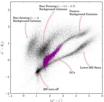
(4) The Astrophysical Journal, 864:36 (23pp), 2018 September 1. Longobardi et al.. based on our high-quality photometric information (see Section 2.3.1). The MMT campaign. In 2009 and 2010, we used the Hectospec multifiber spectrograph on the 6.5 m MMT telescope to survey the compact stellar systems in the central 2°×2° area around M87 (Zhang et al. 2015). Data covered the spectral region within 3650–9200 Å with a resolution of R=1000. By exposing for ∼2 hr, the survey depth is g′∼22.5 mag, and velocities have a typical uncertainty of sVLOS = 30 km s-1. The AAT campaign. Compact objects in Virgo were further followed up spectroscopically in 2012 March/April when we surveyed the central region of the Virgo cluster (Virgo A subcluster) using the 2dF AAOmega multifiber spectrograph on the AAT. Spectra were obtained in the wavelength range 3700–8000 Å and with a spectral resolution of R=1300 (Zhang et al. 2015). The survey consisted of nine 2dF pointings with a typical exposure time of 1.5 hr, covering a total sky area of ∼30 deg2. At the limiting magnitude of g′∼20.5 mag and with such an observational setup, the typical uncertainty on the velocity estimates is sVLOS = 30 km s-1. The Keck campaign. In 2013 April, additional data were collected using the DEIMOS spectrograph located at the Keck II 10 m telescope. The instrumental configuration provided a wavelength coverage of 4800–9500 Å with a spectral resolution of 2.8 Å (FWHM). This campaign provided velocity measurements with a mean precision of sVLOS = 10 km s-1 and down to g′∼24.7 mag (Toloba et al. 2016). Here, 24.7 must be the faintest object, but it is certainly not representative of the GC population. The Magellan campaign. Finally, in 2016 March, we used the IMACS multislit spectrograph on the Magellan Baade telescope to obtain spectra for compact objects in Virgo with g′<22 mag. With a field of view of 27 5×27 5, the observations surveyed two regions, one centered on M87 and the second one offset by 30′ toward the northwest along the major axis of the galaxy. Data were obtained in the wavelength range 3900–9000 Å with a spectral resolution of 6.5 Å. With a total integration time of 3.5 hr, this survey provided data with a mean velocity uncertainty sVLOS = 30 km s-1 (Zhang et al. 2018).. Figure 1. u*i′Ks color–color diagram for the NGVS photometric sample in the pilot region with g′24.0 AB mag. In this plane, background galaxies, GCs, and foreground Milky Way (MW) stars separate into different regions (Muñoz et al. 2014). Magenta dots identify objects with high photometric probability, pgc>0.5, to be GCs (see the text for more details).. The two spectroscopic catalogs with the highest number of GCs in common (67 common objects from the S11 and MMT samples) only present two velocity estimates that deviate by <~1.5 sVLOS. 2.3. Object Classification The selection of a bona fide sample of GCs is a crucial first step for our kinematic analysis. The two main types of contaminants in our sample are (1) background galaxies and (2) foreground Milky Way (MW) stars. A third, more subtle, type of potential contaminant is (3) Virgo UCD galaxies. In what follows, we examine such a contamination and its contribution to the sample of GCs.. As we show below, the NGVS photometry provides vital information needed to select the GC sample that we use to analyze the kinematics of the GC system and identify the LOSVDs of the different dynamical components. Hence our working sample is selected from the matched objects between the NGVS photometric and spectroscopic catalogs in the pilot region, resulting in a total sample of Nobj=2809 sources. We further decide to analyze objects down to g′24.0 mag and sVLOS  50 km s-1. This leads to a total number of sources Nobj=2551, with median photometric uncertainties σmag=[0.01, 0.005, 0.004, 0.005, 0.008, 0.02] in the u* g¢ r ¢ i¢ z ¢ and Ks bands, respectively. Of these objects, 897 have a high photometric probability of being a GC (see Section 2.3.1). Among these, 592 were gathered by S11, while 232, 9, 29, and 18 radial velocities were observed for the first time in the MMT, AAT, Keck, and Magellan campaigns, respectively (the remaining velocities are from public archives). We emphasize that from repeated measurements in different campaigns the velocity estimates are in agreement within the spectroscopic uncertainty threshold of ~sVLOS = 50 km s-1.. 2.3.1. Contamination by Background Galaxies and Foreground Stars. Muñoz et al. (2014) showed that background galaxies, GCs, and foreground stars define different regions in the u*i¢Ks color–color diagram. In Figure 1, this relation is shown for the photometric sample in the NGVS pilot region. From redder to bluer (i′−Ks) colors, we can see the different contributions from background galaxies with various star-forming histories at redshifts up to z;1, GCs (which merge into the redshift sequence of passive galaxies at the red end), and foreground main-sequence stars. However, a successful compilation of a GC sample implies accounting for the shared contribution between different populations in the transition regions of these three sequences. To do so, we have used the full photometric information gathered by the NGVS/NGVS-IR surveys, and we adapted the “extreme deconvolution” (XD) algorithm from Bovy et al. (2011) to classify our data according to multidimensional color and concentration information. The details of this classification procedure will be presented in a future work. Here we give a brief description of the procedure and validate 4.

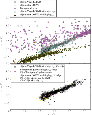
(5) The Astrophysical Journal, 864:36 (23pp), 2018 September 1. Longobardi et al.. Figure 2. Left panel:LOSVD of the spectroscopically confirmed objects in the NGVS pilot region that defines our sample. The GMM best-fit model describes the total LOSVD as a mixture of three Gaussians (black solid line) centered on the star, Virgo ICL, and M87 halo distributions, respectively (black dashed lines). Central panel:BIC and AIC scores for the Gaussian mixtures as a function of the number of components. Both of the information criteria prefer three mixtures to describe the data, as in the left panel. Right panel:posterior probabilities that an object is drawn from one of the three components, that is, the stars (light gray, class 1), the Virgo IC (gray, class 2), and the M87 galaxy (dark gray, class 3) distributions, as a function of its LOSV. For a given velocity value, the vertical extent of each region is proportional to that probability.. of ∼40 km s−1 with a velocity dispersion of ∼120 km s−1 (e.g., Battaglia et al. 2005). Therefore, the MW star LOSVD overlaps with the LOSVD of objects in Virgo, the latter measured to cover a velocity range -500 km s-1  VLOS  3000 km s-1 (Binggeli et al. 1987; Conselice et al. 2001). The contamination by foreground stars is visible as a strong and narrow Gaussian that peaks at around 40 km s−1 in Figure 2 (left-hand panel), where we plot the LOSVD of our working sample with VLOS  3000 km s-1. To isolate this kinematic component, we run a Gaussian mixture model (GMM), that is, a probabilistic model that divides the observed LOSVD into a linear combination of K independent Gaussian probability density functions (PDFs). At the end of the procedure, the posterior probability, Γ, of a data value belonging to either of the K Gaussian components is returned (Figure 2 right-hand panel, and see Section 3 for details on the GMM). Tests with the Bayesian information criterion (BIC) and Akaike information criterion (AIC) show that the GMM best-fit model is a mixture of three Gaussians (Figure 2 central panel), identifying the Galactic stellar contamination as a component with Vstar = 41  4 km s-1 and sstar = 114  3 km s-1. In Section 3, we will show that the remaining two Gaussians are tracing the Virgo cluster and the M87 halo distributions, but because for the moment our goal is to validate the photometric classification, we only isolate the objects with velocities that fall within the stars’ LOSVD, and we consider as one single class the remaining objects. In Figure 3, the (u*−i′) versus (i′−Ks) diagram encodes the spectroscopic information in color: objects with higher GMM posterior probabilities of belonging to the star LOSVD are shown in yellow and orange. From this plot, we can see that the majority of these objects are consistent with being foreground stars on the basis of their u*i¢Ks properties (yellow circles). However, a fraction of objects with u*i¢Ks colors consistent with being GCs have velocities that fall within the star LOSVD. Their total number is 32, that is, ∼4% of the sample of star candidates based. the results in the next section, with the spectroscopic information we have. In the pilot region, the XD approach uses multidimensional Gaussians to model the density of objects in the fivedimensional space: (u*−g′)0, (g′−i′)0, (i′−z′)0, (i′−Ks)0, and a measure of concentration iC = i4¢ - i8¢, where i4¢ and i8¢ are the point source aperture-corrected i-band magnitudes measured in fixed apertures of diameter r=4 pixels (0 72) and r=8 pixels (1 44), respectively. The i-band seeing in the NGVS images has FWHM<0 6 with a median seeing of 0 54. For point-like objects, iC=0, and extended objects have iC>0. The Gaussians in the model are convolved with the observational uncertainties of the data. Therefore, each data point is assumed to be drawn from the model convolved with its own set of measurement uncertainties, and at the end of the XD procedure we obtain for each object the probabilities, pgalx, pgc, and pstar, of it being either a galaxy, a GC, or a star, respectively. Magenta dots in Figure 1 are objects with high photometric probability, pgc>0.5, of being GCs. 2.3.2. Spectroscopic Validation of the Photometric Selection. Background galaxies—There is a well-defined gap between the Virgo members and background galaxies at radial velocities Vgalx = 3000 km s-1 (Binggeli et al. 1987; Conselice et al. 2001; Kim et al. 2014). Therefore, the background component is identified by selecting objects with VLOS > 3000 km s-1. We find that 721 sources in our sample satisfy this criterion, representing ∼28% of our working sample. The XD photometric classification identifies these contaminants successfully: >99% of the background objects are assigned high photometric probability of being background galaxies, with mean value á pgalx ñ = 0.98, and only 1% would result in having high photometric probability of being GCs. Foreground stars—The velocity distribution of the Galactic stellar halo is measured to peak at a heliocentric radial velocity 5.

(6) The Astrophysical Journal, 864:36 (23pp), 2018 September 1. Longobardi et al.. 2.3.3. Virgo UCD Contamination. In the last 20 years, evidence has emerged for the existence of a family of compact stellar systems, called “ultracompact dwarfs” (UCDs). Their sizes and luminosities are intermediate between compact elliptical galaxies and the most massive GCs (Hilker et al. 1999; Drinkwater et al. 2000; Haşegan et al. 2005; Misgeld & Hilker 2011), and their colors and stellar populations are similar to GCs and nuclear star clusters (Taylor et al. 2010; Spengler et al. 2017). Recently, Zhang et al. (2015) studied the properties of a sample of UCD galaxies within ∼1° of M87 and compared them to the properties of the red and blue GC populations. They found that they do not share the same kinematics as the GC system, but no distinction was made between galaxy halo and intracluster GCs, leading to the question as to whether UCDs may trace the IC component instead, hence sharing properties similar to that of the ICGCs. The evidence that the Virgo UCDs never reach the cluster dispersion, nor do they trace the Virgo systemic velocity, is enough to argue that these systems are not to be associated with the ICL. However, the argument gets stronger if we consider that at large radii the UCDs behave more like the red GCs (in terms of density profiles and rotational axis). As we will show in this work (see Section 3), the presence of an IC component particularly affects the GC properties at large radii, and it is dominated by the blue GC population (see Section 4). Thus, if the UCDs did trace the ICL, they would rather show density distributions and kinematics similar to that of the blue GC population at large radii, which we do not observe. We then use the information gathered by Zhang et al. (2015) and Liu et al. (2015) to exclude the UCDs from our sample of bona fide GCs. These authors identified UCDs based on their photometric properties, such as size and colors. By crossmatching the catalogs from Zhang et al. (2015) and Liu et al. (2015) with our sample of compact objects, we identify 85 UCD candidates that we remove from our sample of bona fide GCs. The selection of these objects is reliable, only missing ∼6% of genuine UCDs for g′<21.5 (Liu et al. 2015; Zhang et al. 2015). However, under the assumption that UCDs are the surviving nuclei of tidally stripped galaxies, Ferrarese et al. (2016) argued that we expect a contribution in the 21.5< g′24.0 mag range that amounts to ∼100 objects. Given our spectroscopic incompleteness (on average we only observe 10% of the photometric candidates; see Section 4.2), this implies a residual contamination by UCDs of ∼10 objects in our spectroscopic sample. Such a fraction is negligible with respect to the final sample of GCs and does not affect any of the scientific results that we present in this study.. Figure 3. Top panel: u*i′Ks diagram color coded based on the spectroscopic information: yellow dots are objects with higher posterior probabilities of belonging to the star LOSVD (class 1), while black crosses are more likely to be drawn from the M87 galaxy/ICL distributions (class 2/3). Magenta triangles represent background galaxies. Cyan and orange triangles are objects with velocities consistent with being part of class 1 (orange) or class 2/3 (cyan), but they have photometric probability of being background galaxies. Bottom panel:same as top panel with the object’s size scaled by its photometric probability of being a GC. The photometric information allows us to retrieve the fraction of objects with colors consistent with being GCs but with velocities within the star’s LOSVD (yellow dots). Only 1% of background galaxies (magenta triangles) are misclassified as GCs following the photometric classification.. on their kinematics. In the bottom panel of Figure 3, where the color–color diagram is replotted by weighting the contribution of each data point by the XD probability, pgc, of being a GC, we show that we can successfully retrieve this fraction using the photometric classification previously described. Going back to the top panel of Figure 3, we also see that there are a few misclassified objects (∼9% of our working sample with VLOS  3000 km s-1) with high photometric probability, pgalx, of being background galaxies (cyan and orange triangles). These objects have been visually inspected and reintroduced in the bona fide sample of GCs when their velocity is consistent with the Virgo IC/M87 halo components (cyan triangles, 85 objects). For those whose velocities fall within the star LOSVD (orange triangles, 77 objects), we only reintroduce those that are in the locus of the color–color diagram where the majority of GCs sit (four objects). All of the reintroduced objects have been assigned pgc=1.0. To summarize, we have shown that the photometric information gathered by the NGVS is enough to properly separate foreground stars and Virgo compact objects, allowing us to avoid hard cuts in the velocity distribution for VLOS < 500 km s-1.. 2.3.4. GCs Bound to Other Virgo Members. In the previous sections, we have subtracted the contributions of stars, background galaxies, and Virgo UCDs from our working sample. However, as our goal is to study the GC population of the M87 halo and the Virgo IC component, we also have to flag GCs that are likely to be bound to other Virgo members. To do this, we considered GCs to belong to another galaxy if (1) the GC velocity relative to the galaxy velocity, Vg, is within 3×σg, where σg is the velocity dispersion of the galaxy (assuming a Gaussian LOSVD, 99.7% of the distribution falls within this limit), and (2) their distance from the galaxy’s center is within 10 effective radii, Re, of the galaxy.. 6.

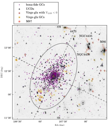
(7) The Astrophysical Journal, 864:36 (23pp), 2018 September 1. Longobardi et al.. This generous radial criterion was chosen to account for possible differences between the galaxy light and the GC spatial distribution. Fits to the SB and surface-density profiles of galaxies’ light and GC systems show that the latter are, on average, more extended than that of the host galaxies’ (e.g., Puzia et al. 2004; Kartha et al. 2014; Forbes 2017; Hudson & Robison 2018). For less-massive dwarf galaxies, the scaling relation can be reduced to Re,GC=1.5×Re,gal (e.g., Peng & Lim 2016). Within a 2° radius around M87, there are 197 Virgo galaxies with known velocity, 129 of which are early-type dwarf galaxies, as compiled by the GOLDMine project (but see also Gavazzi et al. 2003; Toloba et al. 2014). The GOLDMine catalog also provided us the velocity dispersion for a fraction of galaxies, while the effective radius information was retrieved from McDonald et al. (2011). For those galaxies with no measured velocity dispersion or effective radius, mostly dwarfs, we have given a fixed value of sg = 50 km s-1 and Re = 30″. At the end of this procedure, we have identified 56 GCs as belonging to other Virgo galaxies. Finally, we are aware that there will be a fraction of galaxies in the surveyed area with no velocity information, so that is not considered in this analysis. However, we note that additional GCs bound to other galaxies would show a correlation in position and velocity that we checked for. This test showed no evidence of any possible spatial or kinematic correlation, so we can state that if there is a contribution from GCs belonging to other nearby galaxies in our bona fide sample of objects, it is negligible. To summarize, in this section we have analyzed and removed the contribution from contaminants in our working sample to define our final sample of bona fide GCs. We have found the following:. Figure 4. Spatial distribution of GCs in Virgo with spectroscopic information (purple dots) superimposed on the g′-band NGVS image of the Virgo core. Blue triangles show the position on the sky of UCDs, while orange crosses show GCs that we associated with other Virgo galaxies. Aside from M87 (salmon star), we highlight the position of the other four main galaxies as given in the plot. Red crosses identify Virgo galaxies with negative VLOS. The gray ellipses, oriented as the M87ʼs isophotes (major and minor axis inclinations as depicted by the dotted lines), divide the sky into four regions. North is up, and east is to the left.. 1. Background galaxies (i.e., no Virgo members with VLOS > 3000 km s-1) represent ∼28% of our working sample. 2. Once the background contamination is subtracted, foreground MW stars contribute ∼46% of the data, leaving 975 sources with high photometric probability, pgc, of being a compact Virgo object. 3. Among the compact objects, 85, or 9%, are identified as UCDs. 4. Finally, 56 GCs (6% of the total GC sample) are consistent with belonging to other Virgo members.. different PN properties, and hence are consistent with having different parent stellar populations. In what follows, we will investigate whether GCs trace a similar galaxy halo–IC interface. If there are, indeed, ICGCs, in what systems did they form, and do they show photometric properties that differ from the M87 halo GCs? 3.1. Projected GC Velocity Phase Space. This selection led to a final sample of 837 confirmed GCs that we will analyze in the next sections. Their spatial distribution is shown in Figure 4 (purple dots) together with the position on the sky of UCDs (blue triangles) and GCs associated with other Virgo members (orange crosses; the centers of other Virgo galaxies are shown by red crosses).. In Figure 5 we show the velocity–position phase space diagram (central and bottom panels) for our GC sample. The GC LOS velocities are plotted against the major axis distance, the latter computed as R = [(x (1 - e))2 + y 2]1 2 for a system aligned along the y axis, with position angle P. A.=155°. 0 and ellipticity e=0.4 (Ferrarese et al. 2006; Janowiecki et al. 2010). The relations for positive and negative R are plotted separately to trace the northwest (NW; central panel) and southeast (SE; bottom panel) halves with respect to the center of M87, respectively (see Figure 4 for a representation of the spatial configuration). This plot shows a system dominated by random motion, with the GC kinematics concentrated around the M87 systemic velocity Vsys = 1308 km s-1, together with a scattered distribution of high- and low-velocity objects on both sides of the galaxy. As shown in the histograms of the velocities (side. 3. The M87 Galaxy Halo and Virgo ICL as Traced by GCs When studying the light at the center of a cluster reaching out ∼300 kpc (1°) in radius from the central galaxy, we are tracing the transition region between the central galaxy halo and the IC component. Longobardi et al. (2015a) analyzed a 0.5 deg2 area around M87 using PN kinematics to dynamically identify and separate the galaxy halo and the ICL. They showed that the two components overlap at all radii, but with. 7.

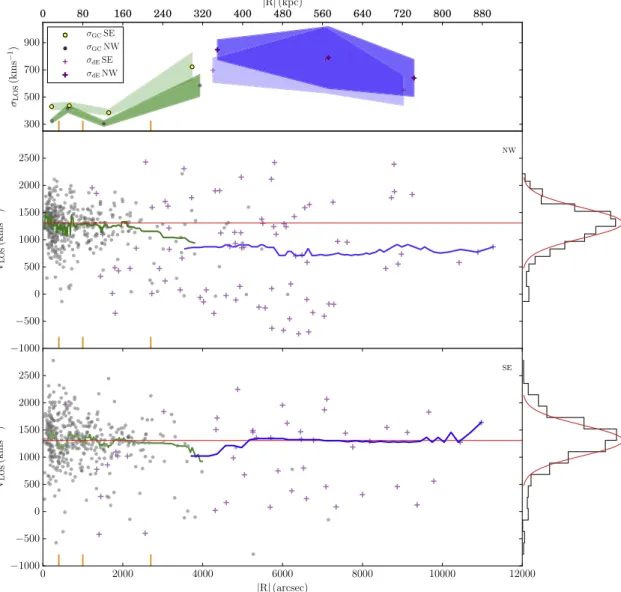
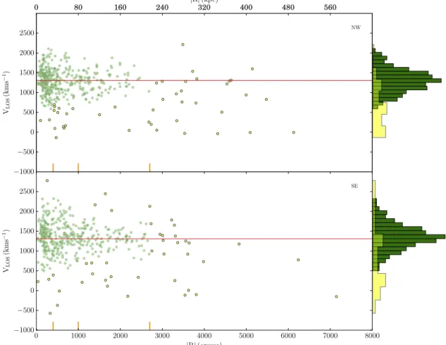
(8) The Astrophysical Journal, 864:36 (23pp), 2018 September 1. Longobardi et al.. Figure 5. Top panel: LOS velocity dispersion profile for the GCs in the NGVS pilot region (dots with the green shaded area delimiting the 1σ region) and for the dwarf early-type galaxies within a 2° radius from the cluster’s center (purple crosses with blue shaded area delimiting the 1σ region). The GC velocity dispersion profile is observed to increase on both the NW (dark dots and dark shaded area) and SE (yellow dots and light shaded area) sides of M87, reaching the velocity dispersion of the dwarfs in Virgo. Central panel: projected velocity phase space that compares the velocity distributions of GCs (black dots) and Virgo dwarf earlytype galaxies (purple crosses) in the NW region. The solid lines trace the running average computed from the total GC sample (green) and the dwarf population (blue). The histogram of the velocities, plotted on the side, shows an LOSVD with strong and asymmetric tails compared to a Gaussian distribution centered on the M87 systemic velocity with a velocity dispersion of ∼300 km s−1 and normalized to the total number of GCs (red curve). Bottom panel:same as central panel, but the relation is shown for the SE region with respect to M87. On both sides, the GC mean velocity decreases as a function of the distances, deviating from the M87 systemic velocity (Vsys = 1308 km s-1, red line) and merging into the mean velocity of the Virgo dwarfs at ∣R∣ ~ 320 kpc . The vertical orange lines separate the phase space into four elliptical bins, as given in the text.. panels), the wings (or tails) of the GC LOSVDs are strong and quite asymmetric with respect to a Gaussian distribution (red curve) centered on the M87 systemic velocity and with a velocity dispersion of σ∼300 km s−1.21 Such behavior contrasts with what is observed for nonrotating early-type galaxies, whose LOSVD are symmetric (i.e., h3∼0) and hence well described by a single Gaussian to within a few percent (Gerhard 1993; Bender et al. 1994). Orbital anisotropy would create a symmetric variation around the mean velocity (i.e., h 4 ¹ 0 ) and is unlikely to be measured at all radii (see Figure 6 for a plot of the GC LOSVDs as a function of the distance from M87ʼs center). On the other hand, strong tails are seen in simulations, observed to characterize the LOSVD of. galaxies in dense environments and consistent with the presence of an intracluster/group component overlapping the galaxy halo (Dolag et al. 2010; Longobardi et al. 2015a; Veale et al. 2017; Barbosa et al. 2018). In fact, the relative importance of these “tails” increases as a function of the major axis distance, with the GCs gradually deviating from the central galaxy’s kinematics and merging into the cluster potential. This is shown in the same plot by comparing the GC kinematics with the kinematics of the population of early-type dwarfs in Virgo with measured radial velocities (129 objects; Gavazzi et al. 2003). We study the running average of the LOS velocities of GCs (solid green lines in the central and bottom panels) and early-type dwarfs (solid blue lines); that is, we plot the running mean in bins of n objects, with n=30 for the GCs, n=35 for the NW dwarfs, and n=25 for the SE dwarfs. By comparing the different runningaverage profiles, it is clear that the GC mean velocity decreases. 21. Here we consider as a velocity dispersion representative of M87 the one traced by the red GC population over a range 0 5–30 0 (Zhang et al. 2015).. 8.

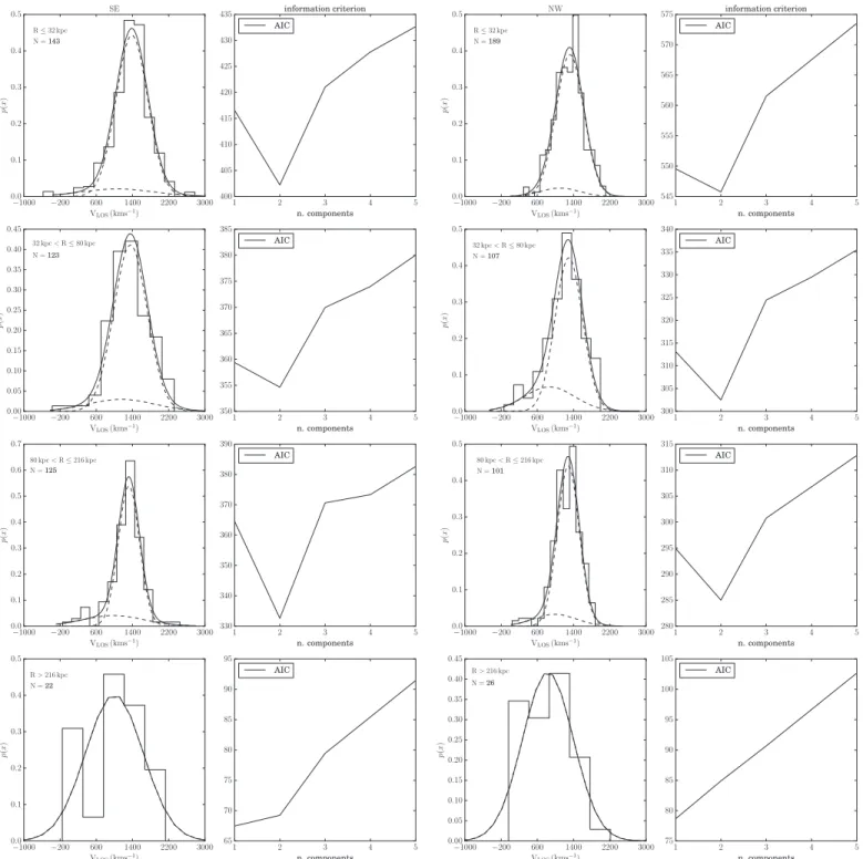
(9) The Astrophysical Journal, 864:36 (23pp), 2018 September 1. Longobardi et al.. Figure 6. GMM analysis of the GC LOSVD carried out separately for the GCs located to the SE (left panels) and NW (right panels) of M87. From top to bottom, the sample is divided into four elliptical annuli as given in Figure 5, with N representing the total number of GCs used in the GMM fitting. An AIC analysis (second and fourth panels) prefers a two-component Gaussian mixture out to R=216 kpc, implying the contribution from the M87 galaxy halo and Virgo ICL to the total LOSVD at all distances out to this radius. For R>216 kpc, the best-fit mixture is a model with one component tracing the Virgo cluster potential.. going toward larger distances, deviating more than 2.5σ at large distances and on both sides from the M87 systemic velocity (red line) and merging into the mean velocity of the Virgo dwarfs at ∣R∣ ~ 320 kpc . At these distances, the GC velocity dispersion reaches its maximum, sLOS = 590  80 km s-1, merging with the cluster potential (Figure 5, top panel). The comparison between the NW and SE fields around M87 shows that the NW has more dE galaxies with negative velocities (red crosses in Figure 4). It is likely that a substantial fraction of these objects comes from the accretion of material that is falling toward the. cluster’s center, dragged along by the well-known infalling M86 subgroup, and it is contributing to what we see today as an IC component. 3.2. Kinematic Separation between the M87 Halo and ICL The comparison with the Virgo dE/dS0 galaxies showed that the GC system around M87 is tracing the transition toward the Virgo cluster potential. Hence, we now further analyze the GC LOSVD, and we do it (1) separately for the NW and SE halves, and (2) in four different elliptical bins, or stripes in 9.

(10) The Astrophysical Journal, 864:36 (23pp), 2018 September 1. Longobardi et al.. Table 1 Fitting Parameters for the GMM Best-fit Models for the M87 Halo and Virgo ICL Components and Separately for the SE and NW Regions NWM87,halo. SEM87,halo. SEICL. NWICL. 1074±403 km s−1 806±285 km s−1 0.10±0.04. 1098±300 km s−1 424±212 km s−1 0.10±0.07. 1153±421 km s−1 729±287 km s−1 0.12±0.07. 865±159 km s−1 551±112 km s−1 0.22±0.06. 977±182 km s−1 680±129 km s−1 0.18±0.05. 986±237 km s−1 474±167 km s−1 0.12±0.06. 999±135 km s−1 634±95 km s−1 1.0±0.2. 833±109 km s−1 559±77 km s−1 1.0±0.2. ∣R∣  32 kpc μ σ W. 1385±30 km s−1 350±21 km s−1 0.90±0.07. 1317±22 km s−1 307±16 km s−1 0.90±0.07. μ σ W. −1. −1. 32 < ∣R∣  80 kpc 1355±34 km s 371±24 km s−1 0.88±0.08. 1293±31 km s 304±22 km s−1 0.77±0.7. 80 < ∣R∣  216 kpc μ σ W. 1319±22 km s−1 234±16 km s−1 0.82±0.08. 1282±24 km s−1 241±17 km s−1 0.87±0.09. ∣R∣ > 216 kpc μ σ W. L L L. L L L. phase space (gray ellipses in Figure 4, or orange lines in Figure 5), covering the entire GC range. The four regions in space are defined as ∣R∣  32 kpc, 32 < ∣R∣  80 kpc, 80 < ∣R∣  216 kpc , and ∣R∣ > 216 kpc, with bin size increasing toward the outer regions to ensure a statistically significant sample of tracers even at large radii, where the GC number density is the lowest. Thus, our choice of radial binning represents the best compromise between similar radial extension and statistical noise. We emphasize that the stability of the results was tested against different choices of radial limits: within the uncertainties, the results are consistent with each other. In our analysis, we assume that both the M87 halo and Virgo IC LOSVDs are Gaussians. As argued in the previous section, this is a reliable approximation for the galaxy’s stellar velocity distribution, and, from hydrodynamical simulations (Dolag et al. 2010; Cui et al. 2014), Gaussian shapes also describe well the IC component. We are aware, however, that a Gaussian may be a less good model for the Virgo IC LOSVD if the Virgo cluster is not fully virialized. We then run a GMM analysis for each of these samples to isolate individual kinematic structures and trace the coexistence of the M87 halo/Virgo IC components. The GMM is a probabilistic model which assumes that a distribution of points, in our case the objects’ velocities, can be described as a linear combination of K independent Gaussian PDFs. The best set of Gaussians is selected by implementing the expectationmaximization (EM) algorithm, an iterative process that continuously updates the PDF parameters until convergence in the likelihood is reached. The process ends with the assignment of posterior probabilities, Γ, that each data point belongs to each of the K Gaussians. This analysis is based on the public scientific Python package scikit-learn (Pedregosa et al. 2011). However, our estimated Gaussian mixture distribution starts from a weighted sample of data, the weights, pgc, being the normalized probabilities of being a GC given its photometric properties (see Section 2.3.1). We then modified the Python GMM routine accordingly, and the details on this. will be given in A. Longobardi et al. (2018, in preparation). Here we only point out that the EM for mixture models consists of two steps. The first step, or E step, consists of calculating the expectation of the component assignments, Γi,k, for each data point given the model parameters. Thus, at the mth iteration of the EM process, the posterior probabilities of the ith particle belonging to the kth Gaussian component become Gim, k =. pk (xi ∣ mk , sk ) Pkm. åk. K. p (x = 1 k i. ∣ mk , sk ) Pkm. ´ pgc, i ,. where the Gaussian density function (PDF) is written as p (xi ) = å kK= 1 pk (xi ∣ mk , sk ) Pk , with pk (x ∣ mk , sk ) being the individual mixture component centered on μk, with a dispersion σk, and mixture weight Pk. The second step, or M step, consists of maximizing the expectations parameters, that is, updating the values μk, σk, and Pk as weighted parameters, the weights being Γi,k. In this way, the EM process always takes into account the starting weight of each particle pgc,i. Tests with the AIC show that the mixture that best describes the total GC LOSVD is a two-component model in the first three elliptical bins, while in the outermost bin, the GMM identifies only one component. A comparison of the performances of AIC and BIC scores was tested against mock sets of data that mimic different LOSVDs and sample sizes. AIC scores were found to be more reliable, so we only report these scores. Moreover, the stability of the fitted parameters was tested with 1000 GMM runs for different mock data sets and initialization values. The results of our GMM analysis, the histograms of the data together with the GMM best-fit model, and relative AIC scores are shown in Figure 6, while we summarize the fitting Gaussian parameters in Table 1. The GMM analysis shows that out to 216 kpc the hotter (broader) and colder (narrower) components coexist, while outside this radius the narrower Gaussian is not detectable, and the GC kinematics are well described by a single broad 10.

(11) The Astrophysical Journal, 864:36 (23pp), 2018 September 1. Longobardi et al.. Figure 7. Top panel: projected velocity phase space that compares the velocity distributions of the M87 halo GCs (green dots) and Virgo ICGCs (yellow dots) in the NW region. The histograms of the velocities, plotted on the side, compare the GC LOSVDs associated with the two dynamical components (green is the M87 halo and yellow is ICL). Bottom panel:same as top panel, but the relation is shown for the SE region with respect to M87. The M87 systemic velocity (Vsys = 1308 km s-1) is plotted as a red line. The vertical orange lines separate the phase space into four elliptical bins, as given in the text.. Gaussian. Within the uncertainties, the narrow Gaussians describe the galaxy’s kinematics with a mean systemic velocity consistent with VLOS = 1308 km s-1, and with a velocity dispersion that decreases as a function of the distance, reaching a value of sLOS ~ 230 km s-1 in the outermost bin. The broad Gaussians, instead, are consistent with the kinematics traced by the early-type dwarf population in the core of Virgo, the latter measured to peak at VdE + dS0 = 1139  67 km s-1, with a velocity dispersion of sdE + dS0 = 649 km s-1 (Binggeli et al. 1993). The mean velocities and velocity dispersions of the ICGC component are consistent not only with those of the dwarf galaxies, but also with those of the more massive systems in the Virgo core (Binggeli et al. 1993). However, (1) very broad, asymmetric wings, like the ones we show in Figures 5 and 6, are only observed for the LOSVD of the dwarf spheroidal galaxies (see Binggeli et al. 1993; Conselice et al. 2001), and (2) in the next sections, we will show that the photometric properties of the detected ICGCs are similar to what is measured for the dE system in Virgo, hence our comparison with the lower mass Virgo galaxies. The broad GC LOSVD component points toward a different kinematic behavior when measured separately in the two halves: SE of M87 the velocity dispersion is larger than in the NW region. However, more kinematic tracers will be needed to reduce the uncertainties associated with these results (see Table 1). For. clarity, the NW and SE GC velocity phase spaces, together with the LOSVDs of the M87 halo and Virgo intracluster GCs, are shown in Figure 7. Different LOSVDs for the galaxy halo and the ICL are predicted by cosmological analysis of structure formation. At the center of simulated clusters, the total LOSVD splits into two Gaussians characterized by very different velocity dispersions (Dolag et al. 2010; Cui et al. 2014). One component is gravitationally bound to the galaxy and more spatially concentrated; the other is more diffuse, and its high velocity dispersion reflects the satellites’ orbital distribution in the cluster gravitational potential. Using this framework, we can identify the narrow and the broad Gaussians traced by the GC kinematics with the M87 halo and Virgo ICL, the latter contributing ∼13% of the GC sample within 216 kpc, beyond which the M87 halo component is no longer detected. In Figure 8 we plot again the comparison between the kinematics of the GC system and the Virgo dE population, but, this time, no separation between NW and SE fields is made. Interestingly, the kinematic behavior of the GC system exhibits a change in dynamics at a projected distance R=128 kpc (see Doherty et al. 2009), where the velocity dispersion reaches its minimum (black dots) and the mean velocity (green line) starts to deviate from the systemic velocity of M87 (red line). Thus, interpreting such a distance as the truncationradius, RT, of the 11.

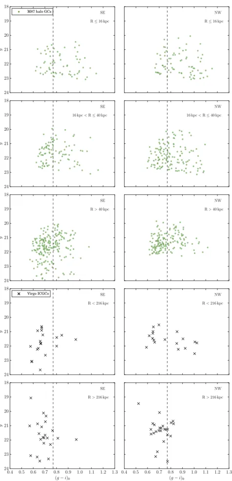
(12) The Astrophysical Journal, 864:36 (23pp), 2018 September 1. Longobardi et al.. 4.1. Photometric Properties Both the M87 halo and the Virgo intracluster GCs are characterized by a large spread in (g′−i′)0 colors, indicating that both dynamical components have two distinct, red (metalrich) and blue (metal-poor), subpopulations of GCs. By fitting a double-Gaussian profile to the GC color distributions, we measure that the red and blue GC components cross at (g′−i′)0=0.77 mag. The relative fraction of blue-to-red GCs differs, however: 77%±10% of the Virgo ICGC population is blue, while only 52%±3% of the GCs bound to the M87 halo are metal-poor.22 In Figure 9, we show the (g′−i′)0 versus g′0 color–magnitude diagram for both the M87 halo (green dots) and the Virgo intracluster GCs (black crosses), separately for the SE and NW fields, and as a function of the distance from the galaxy’s center. The M87 halo sample is compared in three different elliptical bins, while, given the lower number of tracers, the ICGCs are analyzed within two elliptical bins with R=216 kpc representing the boundary. Despite the incompleteness that characterizes our sample of spectroscopically confirmed GCs (higher for R>216 kpc and with the NW side affected the most), we see that the blue GC component of M87 is higher at larger distances, increasing from 40% close to the center to 70% in the outermost bin. This is not true for the IC component that, independently from the distance, is dominated by the blue GCs. We also present the (g′−r′)0 versus (i′−z′)0 color–color diagrams for the M87 halo (Figure 10) and the Virgo intracluster GCs (Figure 11). This analysis was motivated by the recent finding of a correlation between GC color–color relations and environment and interpreted as being driven by different stellar abundance ratios (Powalka et al. 2016b, 2018, although interpretations related to different underlying ages are also given, e.g., Usher et al. 2015; Powalka et al. 2018). In this study, the working sample was selected through a combination of the u*i¢Ks color properties and the compactness of the objects, similar to what we described in Section 2.3.1. However, they only studied GCs whose magnitudes were measured with an uncertainty σmag<0.06 mag in all of the bands, and they also offset the z′ magnitudes to account for known deviations of the SDSS-DR10 magnitudes from the AB magnitude system (Powalka et al. 2016a, 2016b). Hence, we consider the same constraints and restrict our analysis to GCs with the same precision on the magnitude values and apply the same shift to the z′ magnitudes. For each of the color–color diagrams, we fit and plot the relative Gaussian kernel density estimate (kde) and locate its peak identifying the maximum values in (g′−r′)0 and (i′−z′)0 from the kde PDF. The M87 halo GCs are shown in Figure 10 (green dots), where we also flag the position of the blue and red class of GCs as identified based on their (g′−i′)0 values: green dots in red circles refer to the metal-rich population, while green dots in blue circles represent metal-poor GCs. Within R40 kpc, the SE and NW sides of M87 are characterized by GCs with similar colors, with the high-density peaks in the color–color space measured at [(g′−r′)0, (i′−z′)0]SE∼[0.52, 0.15] [0.51, 0.14] and [(g′−r′)0, (i′−z′)0]NW∼[0.54, 0.14] [0.52, 0.15]. Similar are also the distributions of blue and red GCs in the color–color plane. At larger distances, R>40 kpc, the. Figure 8. Comparison between the LOS kinematics of the GCs in the NGVS pilot region and of the dwarf early-type galaxies within a 2° radius from the cluster’s center. At a projected distance R=128 kpc, the GC velocity dispersion (black dots) reaches its minimum, and the mean velocity (green line) starts to deviate from the systemic velocity of M87 (red line). Beyond this radius, the GC kinematics traces the IC potential: the GC velocity dispersion rises until it reaches the velocity dispersion values of the Virgo dE (purple crosses) at R∼320 kpc; at these distances, the GC mean velocity merges into the mean velocity of the Virgo dwarfs (blue line). The mean velocity values are centered on VSys = 1308 km s-1. The error bars show the uncertainties from Poissonian statistics.. galaxy, would imply a total dark matter mass for M87 of MM87 = 4.6 ´ 1013 M. This is a rough estimate, which uses the relation ⎞1 3 ⎛ M M87 ⎟ , RT = RVirgo ´ ⎜ ⎝ 3 ´ MVirgo ⎠. (1 ). were RT = 127.5 kpc ´ ((1 - e)1 2 ) is the average distance within which systems are gravitationally bound to the galaxy, RVirgo is the distance between M87 and the center of the cluster (we have assumed RVirgo=1°; Binggeli et al. 1993), and MVirgo = 4 ´ 1014 M is the total Virgo dark matter mass (McLaughlin 1999). Moreover, we can also speculate that the different velocity dispersions measured for the IC component, higher in the south than in the north, are tracing the unrelaxed nature of the Virgo cluster. Young galaxy clusters still in the process of assembly are expected to show signs of dynamically nonrelaxed substructures. 4. M87 Halo and Virgo Intracluster GC Populations The statistical analysis we have carried out allows us to assign membership to either the M87 halo or the Virgo ICL. In this section, we further analyze the properties of the M87 galaxy and intracluster GCs that have spectroscopic information to investigate whether the different kinematic components also correspond to two different populations in terms of photometric properties and spatial distributions.. 22. Such red-to-blue cluster ratios are consistent with those we would obtain by integrating the extrapolated number density profiles for the red/blue populations related to the two dynamical components (see Section 4.2).. 12.

(13) The Astrophysical Journal, 864:36 (23pp), 2018 September 1. Longobardi et al.. Figure 9. (g′−i′)0 vs. g′ color–magnitude diagram for the M87 galaxy (green dots) and the Virgo intracluster (black crosses) GCs, at increasing distances from the galaxy’s center (see legend) and for the SE and NW halves around M87. As a consequence of the smaller number of objects, the ICGC color–magnitude diagrams are compared in two different elliptical bins, with R=216 kpc being the border. Both dynamical components have a blue and a red population of GCs. In the M87 halo, the number of blue GCs increases as a function of the distance: in the outermost bin it equals ∼70%.. 13.

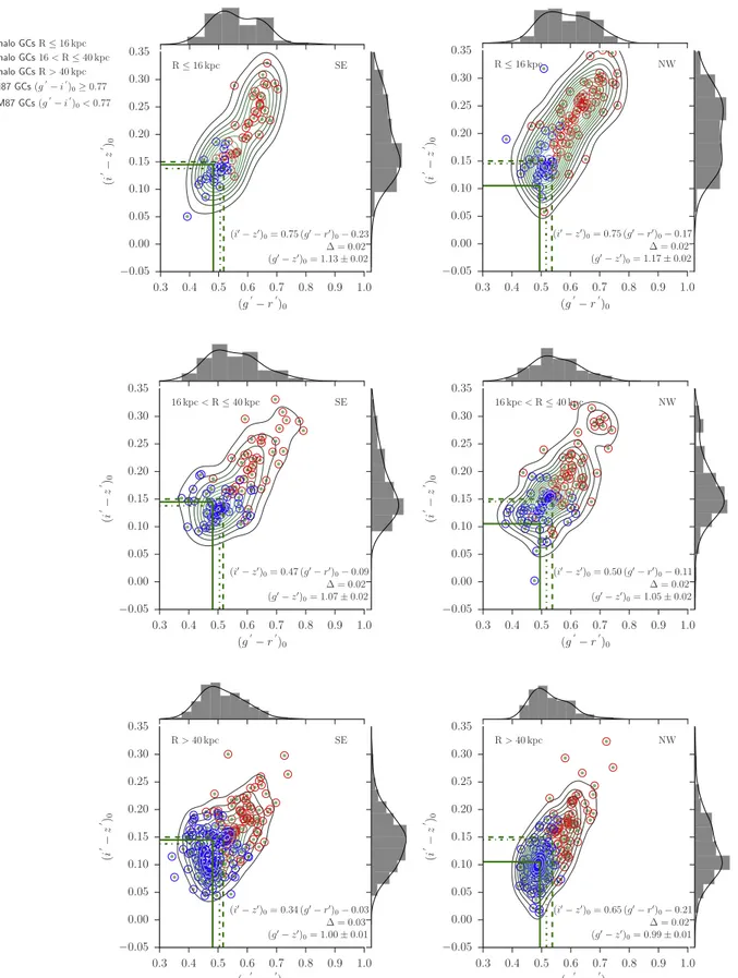
(14) The Astrophysical Journal, 864:36 (23pp), 2018 September 1. Longobardi et al.. Figure 10. (g′−r′)0 vs. (i′−z′)0 color–color diagrams and corresponding kde density contours for the GC populations associated with the M87 halo. Left panel:the relation is shown for the GC population that lies in the SE side with respect to M87, and from top to bottom for GC subsamples at increasing distances from the center of the galaxy. Independent of galactocentric distance, the high-density peaks are close in value, as shown by the green lines. Right panel: same as in the left panel but for the sample of GCs in the NW half of M87. In this region the GCs show bluer (i′−z′)0 colors. In this diagram, we flag the position of the blue and red class of GCs as identified based on their (g′−i′)0 values: green dots in red circles refer to the metal-rich population, while green dots in blue circles represent metal-poor GCs. The linear maximum-likelihood fits to the color–color relations, the Δ values, and the mean (g′−z′)0 colors for each GC subsample are given in the legend. The uncertainty on the magnitudes is less than 0.06 mag.. 14.

(15) The Astrophysical Journal, 864:36 (23pp), 2018 September 1. Longobardi et al.. Figure 11. Same as in Figure 10 but for the Virgo ICGCs. The ICGCs are characterized by bluer colors than the galaxy GCs (the green dashed line shows a representative peak at [(g′−r′)0, (i′−z′)0]∼[0.51, 0.14]), with the bluest population found at R>216 kpc. The magenta dashed lines show the color–color highdensity peak for a sample of GCs associated with Virgo early-type dwarfs. The linear maximum-likelihood fits to the color–color relations, the Δ values, and the mean (g′−z′)0 colors for each GC subsample are given in the legend. The uncertainty on the magnitudes is less than 0.06 mag.. color–color diagram extends to bluer (i′−z′)0 colors, with a significant fraction of objects with (i′−z′)00.1. We note, however, that the average behavior differs between the SE and NW regions. NW of M87 the blue GCs define the high-density peak in the color–color diagram at [(g′−r′)0, (i′−z′)0]∼[0.50, 0.11]. SE of M87 the blue GC population occupies a larger area, and the high-density peak is measured at [(g′−r′)0, (i′−z′)0]∼[0.48, 0.14]. The same analysis is carried out for the ICGC sample (we use the same binning as in Figure 9). The results are presented in Figure 11, where this time black dots in red and blue circles identify the metal-rich and metal-poor populations of GCs, respectively. The ICGC concentration in the color–color space differs from the one observed for the M87 halo GCs: independently from the distance, a large fraction of ICGCs extend to (i′−z′)00.1, the distribution is dominated by the blue ICGCs, and the few red GCs are bluer in the (g′−r′)0 versus (i′−z′)0 plane. This implies blue high-density peaks measured at [(g′−r′)0, (i′−z′)0]SE∼[0.44, 0.12] [0.48,0.11] and [(g′−r′)0, (i′−z′)0]NW∼ [0.47, 0.13] [0.49,0.07]. These are bluer than the one measured for. the M87 halo GCs, of which we show a representative peak as a green dashed line. We also compared the ICGC color–color distribution with the one measured for the 33 GCs that in Section 2.3.4 we identified as being bound to Virgo early-type dwarfs. Their peak (magenta dashed line in Figure 11) is measured at redder colors. Besides the offset in the color peaks, the comparison between Figures 10 and 11 also shows different slopes for the M87 halo and Virgo intracluster GCs color–color relations. A maximum-likelihood linear fit to the (g′−r′)0 and (i′−z′)0 results in a galaxy component that is usually steeper than the ICL. Also, by computing the median deviation of the GC (i′−z′)0 colors from the fitted linear relation, Δ, the locus of the M87 halo GCs is tighter (i.e., stronger color–color relation) than the one of the ICGCs (fitted parameters and Δ values are given in the legends of Figures 10 and 11). Such properties can be interpreted in terms of different metallicity distributions (Powalka et al. 2016b). Finally, Peng et al. (2006) find that the mean (g′−z′)0 colors of the GCs in ACSVCS galaxies define a color–magnitude sequence, such that more luminous or massive galaxies host, on 15.

(16) The Astrophysical Journal, 864:36 (23pp), 2018 September 1. Longobardi et al.. average, redder GC systems. We than computed the mean (g′−z′)0 colors for the M87 halo and Virgo intracluster GCs and as a function of the distance. The GC systems bound to the M87 halo show redder mean (g′−z′)0 values. Averaged across the distance, and with no distinction between NW and SE halves, we find <(g′−z′)0,M87>=1.07±0.01, while for R>40 kpc we find <(g′−z′)0,M87>=1.00±0.01. The Virgo ICGCs are constant, within the uncertainties, to a mean color <(g′−z′)0,IC>0.94±0.02. Such a result is consistent with the galaxy-accreted component dominating the outer regions and reinforces our conclusion that the ICL is built up by less massive systems than the one contributing to the size growth of the M87 halo. 4.2. Density Profiles We are now interested in studying the spatial distributions of the M87 halo and Virgo intracluster GCs to analyze their density profiles. This is because differences in their radial profiles may imply differences in the evolutionary paths of these two components as different progenitors are expected (Dolag et al. 2010; Cui et al. 2014) and observed (Longobardi et al. 2015a) to contribute differently to the resulting density distribution.. Figure 12. Spatial distribution of the velocity-selected sample of GCs (green dots are M87 halo GCs and yellow dots are ICGCs) superimposed on the g′band NGVS image of the central 2 by 2 square degrees of Virgo. The NW field is more affected by spatial incompleteness. East is to the left, and north is up.. 4.2.1. Spatial Completeness. In order to analyze the GC density profiles, we need to compute a completeness factor as a function of the distance, Cspec (R), that accounts for the spatial incompleteness of our spectroscopically selected sample of GCs. Such a completeness is estimated against the photometrically selected GCs, that is, objects with high pgc probability (see Section 2.3.1), that we recall being 100% complete down to our limiting magnitude, g′=24.0 mag. We then estimate the completeness function by computing the ratio between the number of photometric GCs with spectroscopic information, NGC,spec, and the total number of GCs in the photometric sample, NGC,phot, in each elliptical annulus.23 Hence, the completeness factor as a function of the distance from M87ʼs center, Cspec (R), can be written as Cspec,j (R) =. NGC,spec,j NGC,phot,j. 4.2.2. Density Profile for the M87 Halo and Virgo Intracluster GCs. The density profiles for the M87 halo and intracluster GCs are constructed by binning our GC samples in elliptical bins that have as major axis distances the same as what we used for our GMM analysis in Section 3 (see also orange lines in Figure 5) and as position angle and ellipticity P.A.=−25°. 0 and e=0.4, respectively (Ferrarese et al. 2006; Janowiecki et al. 2010). Hence, for each of the two dynamical components of GCs and as a function of the distance, the density is computed as r M87,j (R) =. ,. r ICL,j (R) =. where R is the average major axis distance of all GCs falling within each elliptical annulus. The subscript j indicates the two different GC components, red and blue. Averaged over the elliptical bins, the completeness factor amounts to áCspecñ = 0.1, but the NW field is more affected by incompleteness than the SE region. This effect is measured at larger distances so that in the last bin we miss 40% more GCs NW of M87 as compared to the SE. This is due to observational strategies that observed the SE region more, but it is also related to the fact that the NW region has more photometric objects per unit area. In Figure 12 the sky positions of our sample of data (both M87 halo, green dots, and Virgo intracluster GCs, yellow dots) can be seen overplotted on the NGVS g′-band image.. (Nobs,M87,j (R) - Nov,j (R)) A (R ) (Nobs,ICL,j (R) + Nov,j (R)) A (R ). ´ ´. 1 Cspec,j (R) 1 Cspec,j (R). ,. (2 ). (3 ). where Nobs,M87(R)/Nobs,ICL(R) is the observed number of M87 halo and Virgo intracluster GCs in the elliptical bin, respectively; A(R) is the annulus area, estimated via Monte Carlo integration techniques if only a portion of the annulus intersects our FOV, and Cspec (R) is the spectroscopic completeness factor. The observed numbers of clusters together with the completeness factor differ for the two, red and blue, populations of GCs, which in Equations (2) and (3) are denoted with the subscript j. As can be seen in Figure 6, the ICL and M87 halo velocity distributions overlap, and as a result, the GMM algorithm assigns the ICGCs at low velocities relative to the galaxy systemic velocity to the galaxy halo component. We statistically quantified this effect by comparing the M87 halo and IC velocity distributions in each elliptical bin. The LOSVDs of the two components were approximated by Gaussian functions with mean values and dispersions as given in Table 1. Hence, we calculated the fraction of ICGCs that lie inside the galaxy halo distribution as the area of overlap. 23 The completeness function Cspec (R) is computed using the spectroscopic sample of objects retaining those GCs that we flagged as bound to other Virgo members. This is because the photometric sample of GCs we use to complete our observations does contain such a contribution, and in this way the ratio is still conserved.. 16.