Three layer thermal model to measure the heat capacity of metallic thin films

Texto completo

(1)Three-layer thermal model to measure the heat capacity of metallic thin films J. O. Noveloa,b, R. D. Maldonado a*, A. I. Oliva a,1, A. Hurtadob a. Universidad del Mayab, Facultad de Ingeniería. Carretera Mérida-Progreso Km. 15.5, A P 96, Cordemex, CP 97310, Mérida, Yucatán, México. b Centro de Investigación en Materiales Avanzados S. C, Departamento de Física de Materiales, Av. Miguel de Cervantes 120, Complejo Industrial Chihuahua, CP 31109 Chihuahua. Chihuahua, México. *ruben.dominguez@anahuac.mx Abstract Nanotechnology applications have become a reality in some materials science fields. Thermal properties of metallic nanofilms reported in the literature have shown to posses different values as compared with their bulk properties. The determination of the thermal properties plays a key role in the design of components and in the production of new materials. In this work a new method to estimate the heat capacity of metallic thin films is discussed. The analyzed thermal model consists in a three-layer system formed by a film/substrate/film. To estimate the heat capacity of the metallic film, it is required to apply a constant dc current in one metallic layer such that the three-layer system reaches the steady-state. In this condition, a dc current pulse is applied in the same metallic layer acquiring in real time the corresponding voltage and the changes of temperature as a consequence of the applied pulse. The three-layered model is analyzed by using coupling differential equations which includes the different mechanisms of heat transfer involved as a function of the physical properties and the geometrical parameters. Simulated results obtained from Au/glass/Au, Al/glass/Al, and Cu/glass/Cu systems for different electrical pulses and film thicknesses are discussed. These analytical results provide tools for developing better experimental conditions to estimate the heat capacity of metallic nanofilms. Keywords: thermal model, three-layer, heat capacity, metallic films 1. INTRODUCTION The understanding of the thermodynamic properties of materials at nanoscale has become important in the development of new technological applications. Heat capacity provides basic information about the physical properties of the materials. Electronic, magnetic and structural properties can be studied by knowing the heat capacity parameter. Various experiments and models have been proposed for measuring the heat capacity: thermal relaxation method [1], thinfilm DSC nanocalorimetry (TDSC) [2] and curve fitting method (CFM) [3], among others. The thermal relaxation method used to measure the heat capacity in materials it has been used for many years. This method consists in the observation of the increment of temperature during the sample heating with a pulse of current applied to a system [4]. One of the most important advantages of this method is its simplicity, but the experimental conditions should be close to be an adiabatic system. Several theoretical models and experimental techniques have been proposed to estimate the heat capacity of films as a function of the temperature and the thickness in adiabatic conditions. However, these models and techniques do not take into account convection and radiation effects [5-10]. In this work, we proposed a thermal model to estimate the heat capacity in thin metallic films considering, both radiation and convection effects, such that heat capacity of films can be obtained. 1. On leave from Cinvestav IPN Unidad Mérida, Applied Physics Department. (oliva@mda.cinvestav.mx).

(2) at room conditions and atmospheric pressure. Also, the proposed model can help us to clarify new experimental conditions to measure the heat capacity in metallic films with nanometric scale. 2. THEORY Figure 1 describes the system analyzed in this work. The thermal and geometrical parameters used for modeling are described. A balance of energy in Figure 1 needs to obey: =(. +. +. ). ( ). ). +(. ( ). +(. +. +. ). ( ). (1). = , is the power applied to the metallic film deposited under the substrate. We define where as the additional pulse of energy applied to the same metallic film in steady conditions which is is the step function activated in time and defined as = [ ( − ) − ( − )] where = + is divided deactivated in time such that − is the pulse of time. The total energy between the two films and the substrate. The heat transfer mechanisms involved in Eq. (1) are defined as: = ( − ), = ℎ ( − ) and = − , which are the sensible heat and heat losses by convection and radiation respectively. Subscript could be , , ℎ , , ; are the changed by the film (1), substrate (2) and film (3). Constants , , , voltage, the applied electrical current, the mass, heat capacity, room temperature, convection coefficient, area, emissivity of each layer of the system and , is the Stefan-Boltzmann constant.. Figure 1. Schematic diagram and heat transfer mechanism of the three-layer model analyzed in this work. Terms of Eq. (1) can be separate in three parts, according with each component. Dividing the energetic contributions for each part, we can write: ) + =( + + =( ) + ( ) ) =( + + (. ( ). +. ). for film (1) for substrate (2) for film (3). (2). and are the heat conduction through the substrate (2) and film (3), respectively and Where are defined as follows: =. (. −. ). and. =. (. −. ). (3).

(3) Constants , , and are the thermal conductivity, area, thickness and temperature of the and are the thermal conductivity, area, thickness and temperature of the substrate (2); , , film (3). Substituting each component of the heat transfer mechanisms in the system of equations (2) and defining a new group of variables, we obtain a first order differential equations system with three variables similar to the reference [11] for a bimaterial system: ( )+ ( )− ( )= + ( )+ ( )− ( )− ( )+ ( )−. [ ( − ) − ( − )] ( )=0 ( )=0. (4). Here, subscripts 1, 2 and 3, refer to the lower film, the substrate, and the upper film of the system, respectively. Variables ( ), ( ) and ( ) are the changes of temperature with time of the different layers defined as follows: ( )= ( )= ( )=. ( )− ( )− ( )−. (5). With the initial conditions: (0) = 0 (0) = 0 (0) = 0. (6). Constants in Eq. (4) are defined as: =. ℎ. +. +. ;. =. =. =. + ℎ. +. ;. ;. =. +. ;. =. ;. ;. =. =. ; (7). =. and are included the radiation effects and the temperature is defined in In the parameters and defined in Eq. (7) as absolute values. Thus, the constants = [(. + 273) + (. = [(. + 273)][(. + 273) + (. + 273) + (. + 273)][(. [( + )( + )− {[( + )( + )−. ][ + ( − ]( + )−( +. (8). + 273) ]. + 273) + (. ( ), Applying the Laplace transform method (LTM) and solving for Wolfram Mathematica* Ver. 7 software, Eqs. (4) can be transformed to: ( )=. + 273) ]. ( ) and ) ). ] }. ( ) with the.

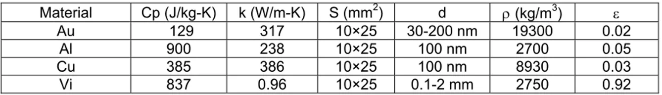
(4) ( )=. {[. − ( + )( )( + −( +. {[. − −( +. +( − ) ) )]( + )+( +. ). } (9). ( )=. (. +( − )( + )]( +. ) ) )+( +. ). }. Equations (9) were numerically solved to obtain the thermal profiles in the system according to the initial conditions proposed. The profiles of temperature with time were obtained by applying the inverse Laplace transform. Each one of the three solutions is composed by tenths of terms and is not shown in this manuscript but the thermal behavior in the three-material system can be predicted as exponential functions according to: / / ( )= + + / / ( )= + + (10) / / ( )= + + y . These constants The exponential functions in Equations (10) involves two times constant represent the relaxation time for the film and for the complete system respectively. However, the plot of each one under different conditions will be discussed in the Results section. 3. RESULTS Table 1, shows the bulk physical properties and dimensions used to simulate the thermal profiles in the three-material system. All simulations were realized varying these parameters: film thickness, substrate thickness, heating time pulse and the power applied to the three-layer system. Table 1. Physical bulk properties and geometrical parameters used in thermal profiles simulations for the three-layer system. Material Au Al Cu Vi. Cp (J/kg-K) 129 900 385 837. k (W/m-K) 317 238 386 0.96. S (mm2) 10×25 10×25 10×25 10×25. d 30-200 nm 100 nm 100 nm 0.1-2 mm.  (kg/m3) 19300 2700 8930 2750.  0.02 0.05 0.03 0.92. Typical simulated temperature profiles are presented in Figure 2. In these figure the bimaterial system [12] is compared with the three-material system. For the bimaterial case, two thermal profiles are show corresponding to the film (upper) and for the substrate (lower). The convection coefficient value used in all simulation was always 19.9 W/m2°C. This magnitude of the coefficient represents typical value for natural convection [13]. Both profiles were obtained under the same conditions. From this figure it can be see that the two systems reach the steady state after 250 s. The temperature in steady state in the bimaterial system is higher than the obtained with the threematerial system, indicating that the global coefficient in the three-layer system is higher than for the bimaterial system. Figure 3 present different temperature profiles with different powers applied to the three-material system. A linear increment on the temperature of the thermal profiles was found with the increase of the power applied in the three-layer model..

(5) 16. bimaterial system. 10. 14. 2. Q0=0.1 W, h1=h2=19.9 W/m °C. 8. Three-material system. 10. 2. Q0=0.08 W, h1=h2=19.9 W/m °C. 8. Xfilm-Au [11]. 6 4. Au/glass/Au (0.5 m/1 mm/0.5 m) Q0 = 0.0985 W. 2. h= 19.9 W/m °C. 0 0. Xglass [11]. 100. X2(t) X3(t) 2. Q0=0.05 W, h1=h2=19.9 W/m °C. 4. Au/glass/Au (0.5 m/1mm/0.5 m). X2(t). 2. 2. Q0=0.02 W, h1=h2=19.9 W/m °C. X3(t) 150. 200. time (s). Figure 2. Theoretical simulated with the Au/glass/Vi.. X1(t). 6. X1(t). 2. 50. Xi (°C). Xi (°C). 12. 2. 250. 0 0. 300. Q0=0.01 W, h1=h2=19.9 W/m °C. 100. 200. 300. 400. 500. 600. time (s). temperature three-layer. profiles system. Figure 3. Heating profiles for the Au/glass/Au system for different applied power.. When the system reaches the thermal stabilization, a heating pulse is applied over the first signal of the three-material system. Figure 4 shows the thermal profiles obtained for different heating pulses. The heating pulse applied in the three-material systems was 1, 5 and 10 s. An exponential decay was found in the simulated profiles. All profiles reach the stationary state after 300 s approximately. Heating profiles for different applied power are presented in Figure 5. The applied power in each three-layer system was 0.2, 0.5 and 1 W. These profiles reach the thermal stabilization once again after 300s. 30. 12. Au/glass/Au (0.5 m/1 mm/0.5 m) Q0 = 0.1 W, Q1 = 0.2 W 2. h= 19.9 W/m °C. 10. 27. Xi (t). X2(t). 24. X2(t). X3 (t). 21. X3 (t). t=5 s. 12.5. 6 4. t=1 s. 10.0 520. 0 0. 200. 400. 560. 600. time (s) 600. time (s). 640. 800. Q1=0.2 W. 15. 9. 11.0 10.5. 2. Q1=0.5 W. 12. 12.0 11.5. Q1=1 W. 18. t=10 s. 13.0. Xi (t). Xi(t). 13.5. 8. Xi (t). Xi(t). 14. 680. 1000. Figure 4. Theoretical thermal profiles simulated with different heating pulses. All simulations reach the stabilization at 300 s approximately.. 6. Au/glass/Au (0.5 m/1 mm/0.5 m) Q0 = 0.1 W, t=10 s. 3. h= 19.9 W/m °C. 0 0. 2. 200. 400. 600. 800. 1000. time (s) Figure 5. Heating profiles for different applied power pulses. The stationary state is reached after 300 s approximately.. Figure 6 shows the exponential fitting of the thermal profiles by using the Equations 9 in order to obtain the relaxation constant time of the complete system . This relaxation time constant was found for this case found when the system reaches the 63.2% of the stationary state. The value was 58.44 s. This value does not change with the time of the heating pulse and with the power pulse applied to the three-material system. The Figure 7 presents the time constant behavior for the three-layer system as a thickness substrate function. The time constant increases linearly with the.

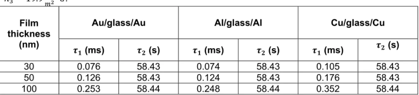
(6) thickness of the substrate in the three-material system due to increase of amount of mass in the substrate. 14. 120. 2=58.44 s. 12. time constant 2 (s). 100. 10. Xi (t). 8 6 4. X1(t). Au/glass/Au (100 nm/1 mm/100 nm) Q0 = 0.01 W, Q1 = 0.02 W, t=10 s. X2(t) X3(t). 2. h= 19.9 W/m °C. fitting 2. 2 0 0. 200. 400. 600. time (s). 800. 80 60 Au/glass/Au (100 nm/d2/100nm). 40. Q0 = 0.01 W, Q1 = 0.02 W, t=10 s 2. 20. h= 19.9 W/m °C. 0 0.0. 1000. 0.5. 1.0. 1.5. 2.0. glass substrate thickness (mm). Figure 6. Fitting for the three-material thermal found for profiles using the Equations 9. The this case was 58.44 s.. behavior Figure 7. Relaxation time constant varying the glass substrate thickness. The thermal profiles were simulated under the same conditions. Figure 8 shows the thermal profiles during the first milliseconds of heating of the three-material system. In this short time we assumed that the substrate remains at the same temperature and the heating pulse does not affect the substrate. When these system conditions are given a new relaxation time constant of the film can be found. This time constant represent the first instants of the film heating. Adjusting the thermal with Equations 9, we found a relaxation time constant of = 0.253 for the Au/glass/Au analyzed. The Figure 9 shows the relaxation time constant varying the film thickness. A linear behavior was also found between the relaxation time constant and the thickness of the film. 0.5. 0.5. film time constant 1 (ms). 0.4. X1(t) X2(t). Xi (t). 0.3. X3(t). 1=0.253 ms. 0.2. Au/glass/Au (100 nm/1mm/100nm) Q0 = 0.01 W, Q1 = 0.02 W. 0.1. 2. h= 19.9 W/m °C 0.0 0.0. 0.4. 0.8. substrate 1.2. 0.4. 0.3. 0.2. Au/glass/Au (d1/1 mm/d3) Q0 = 0.01 W, Q1 = 0.02 W 2. h= 19.9 W/m °C. 0.1. 1.6. 2.0. time (ms). Figure 8. Thermal profiles of the first 2 ms of heating in the three-material system showing the relaxation time constant .. 30. 60. 90. 120. 150. 180. 210. fim thickness (nm). as a Figure 9. Relaxation time constant function of the thin film thickness during the first 2 ms in the three-material system.. and obtained for different three-material systems: Table 2 shows the simulate results of and are presented as a Au/glass/Au, Al/glass/Al, Cu/glass/Cu. The relaxation time constant function of the film thickness. All three-material systems were simulated under the same conditions..

(7) Table 2 shows that the relaxation time constant are independent of the film material analyzed and independent of the film thickness given that its mass is more smaller than the mass of the substrate. When the first two milliseconds is analyzed in the three-material system, changes with the film thickness and the three metallic films analyzed shows different behaviors in the relaxation time constant. Table 2. Time constants ( and ) obtained for different three-material systems. The systems =1 , = 0.01 , = 0.02 , ℎ = analyzed were simulated using the same conditions: ℎ = 19.9 ° . Film thickness (nm) 30 50 100. Au/glass/Au (ms) 0.076 0.126 0.253. Al/glass/Al (s). (ms). 58.43 58.43 58.44. 0.074 0.124 0.248. Cu/glass/Cu (s). 58.43 58.43 58.44. (ms) 0.105 0.176 0.352. (s) 58.43 58.43 58.44. By knowing the initial slope of the heating (or cooling) profile corresponding to the film ( ) it is ∆ /∆ , then: possible to estimate the specific heat of the metallic film if we consider that = =. (∆ /∆ ). (11). 4. CONCLUSIONS We present a thermal model to simulate the thermal profiles in three-material systems. This model allows obtaining the relaxation time constant for the thin film and the relaxation time constant for the complete system. These results are the first steps in the development an experimental method to and . The experimental challenge is to implement a method to generate a micropulse obtain (about 2 ms) and acquire the thermal profiles with high resolution (about 1 data per microsecond). From these experimental results we will be able to estimate the heat capacity of nanofilms by knowing the thermal profiles of the three-layer systems. 5. REFERENCES [1] Jun Yu, Zhen’an Tang, Fentian Zhang, Haitao Ding, Zhengxing Huang, Journal of Heat Transfer, 132 (2010) 012403 [2] M. Yu. Efremov, E. A. Olson, M. Zhang, S. L. Lai, F. Schiettekatte, Z. S. Zhang, L. H. Allen, Thermochimica acta, 407 (2004) 13-23. [3] Jih Shang Hwang, Kai Jan Lin, Cheng Tien, Rev. of Sci. Instrum., 68 (1997) 94-101. [4] A. G. Worthing, Phys. Rev., 12 (1918) 199. [5] D. R. Queen, F. Hellman, Rev. Sci. Instrum., 80 (2009) 063901. [6] Ki Sung Suh, Hyung Joon Kim, Yun Daniel Park, Kee Hoon Kin, Journal of the Korean Physical Society, 4 (2006) 1370-1378. [7] Jon P. Shepherd, Rev. Sci. Instrum., 56 (1985) 273-277. [8] Aitor F. Lopeandía, F. Pi, J. Rodríguez-Viejo, Appl. Phys. Lett., 92 (2008) 122503. [9] M. Brando, Rev. Sci. Istrum., 80 (2009) 095112. [10] Eric A. Olson, Mikhail Yu. Efremov, Ming Zhang, Zishu Zhang, Leslie H. Allen, Journal of Microelectromechanical Systems, 12 (2003) 355-364. [11] R. D. Maldonado, A. I. Oliva, H. G. Riveros, Surf. Rev. Lett., 13 (2006) 557-565. [12] A. I. Oliva, R. D. Maldonado, O. Ceh and J. E. Corona, Surf. Rev. Lett., 12 (2005) 289-298. [13] F. Kreith, M. S. Bohn, Heat Transfer Principles, Ed. Thomson-Learning, 2001..

(8)