Magneto rheological damper modeling using LPV systems

Texto completo

(1)INSTITUTO TECNOLÓGICO Y DE ESTUDIOS SUPERIORES DE MONTERREY MONTERREY CAMPUS. GRADUATE PROGRAM IN MECHATRONICS AND INFORMATION TECHNOLOGIES. MAGNETO-RHEOLOGICAL DAMPER MODELING USING LPV SYSTEMS THESIS SUBMITTED TO INSTITUTO TECNOLÓGICO Y D E ESTUDIOS SUPERIORES D E M O N T E R R E Y IN PARTIAL F U L F I L M E N T OF T H E R E Q U I R E M E N T S FOR T H E D E G R E E OF. MASTER OF SCIENCE IN AUTOMATION BY. VICENTE ALBERTO DIAZ SALAS M O N T E R R E Y , N U E V O LEÓN, MÉXICO , J A N U A R Y 2011.

(2) ©Copyright by Vicente Alberto Diaz Salas, 2011 All Rights reserved. ii.

(3) INSTITUTO TECNOLÓGICO Y DE ESTUDIOS SUPERIORES DE MONTERREY MONTERREY CAMPUS. The committee memberes hereby recommend the thesis presented by Vicente Alberto Díaz Salas to be accepted as a partial fulfulment of the requirements for the degree of M A S T E R O F S C I E N C E IN A U T O M A T I O N. Director of Electronic and Automation Gradúate Programs I T E S M , Monterrey Campus. Monterrey, Nuevo León, México, January 2011.. 111.

(4) MAGNETO-RHEOLOGICAL DAMPER MODELING USING LPV SYSTEMS. BY. VICENTE ALBERTO DIAZ SALAS. Presented to the Graduate Program in Mechatronics and Information Technologies. This Thesis is a partial requirement for the degree of Master of Science in Automation. Instituto Tecnológico y de Estudios Superiores de Monterrey. Monterrey, Nuevo León, México , January 2011. iv.

(5) External Advisors. Acknowledgements. Olivier Sename I would like to thank Dr. Olivier Sename for his fundamental support in this research project before, and during the stay at GIPSA Lab; his advices in the design process of the L P V model were fundamental to complete this work, and his great support allowed me to achieve the stay at France, which was a grateful experience in my professional and personal life.. Luc Dugard I also owe my deepest gratitude to Dr. Luc Dugard for his great support and encouraging during my stay at Grenoble, his advices were very important to finish the L P V model, and his good spirit aided me to keep on in the working process of the research. It was an honor being part of the automotive group at GIPSA.. v.

(6) Acknowledgements. It is a pleasure to thank the many people who made this thesis possible. First of all I would like to thank my advisor Dr. Ruben Morales Menendez for his guidance trough all the research project in which I was involved, for his patience to complete this thesis, and his help to improve my work during all the time I was under his supervision, without his aid this work simply would not have been done. Besides my advisor, I would like to thank the rest of my thesis committee: Dr. Ricardo Ramirez for his help to involve me in the research project and his support for being part of GIPSA Lab, at Grenoble. Also Dr. Luis Eduardo Garza for his encouragement, insightful comments, and hard questions to complete this work. Special thanks to Jorge Lozoya for his help during the beginnings of my work which resulted in the paper: "Building Training Patterns for Modelling M R Dampers" at the 7th International Conference on Informatics in Control, Automation and Robotics 2009 in Milan, Italy, and for his encouragement to be part of the experimentation project. Also to Ing. Ricardo Prado Gamez because his support during the experimental tests at summer 2009. I also thank Javier Ruiz from Tec de Monterrey and Do Ahn Lam from GIPSA Lab for his great collaboration and friendship during this research project, without their help and encourage¬ ment it would not have been possible to achieve the results presented in this work. I am indebted to my many student colleagues for providing a stimulating and fun environ¬ ment in which I was able to study; I am especially grateful to Juan Carlos Tudon, Deneb Robles, Luis Sandoval, Denisse Sandoval, Dulce Aguilar, Juan Rubio, Guillermo Lopez, Diana Tor¬ res, Violeta Casillas and to Roberto Cruz from TEC, and to Federico Bribiesca, Lizeth Torres, David Hernandez, Francisco Marquez, Luis Olmos, Simona Mihaita, Andra Vasiliu, Irfan Ah¬ mad, Oumayma Omar, Antoine Lemarchand, and Joumana Hermassi from GIPSA Lab.. vi.

(7) Dedication. A mi Familia, el regalo mas importante que me ha dado Dios: mis padres, a quienes les debo todo lo que soy y a quienes quiero con toda el alma; mis hermanos, quienes siempre me han dado todo su apoyo; mis sobrinos Rafa, Lucero y Lupita, quienes me ayudaron a seguir trabajando con su buen humor e inspiration.. vii.

(8) Abstract. The present research is focused in the dynamical modeling of a Magneto-Rheological Damper as a semi-active actuator. This device shows a complex behavior including non-linearities and hysteresis, features that are to be emulated by a dynamical system, in order to express mathematically the conduct of this device under mechanical vibrations. The M R damper is part of a semi-active suspension system, and by the use of the information of the model designed in this thesis it might be possible to produce a control design for the quarter of car system, in order to regulate the vibrations received by the suspension, incrementing the comfort and safety of the passengers in the vehicle. In order to obtain experimental data from this semi-active device, a set of tests were performed, introducing displacement and current excitation patterns into the shock absorber and measuring the dynamical response of it. Using the experimental results, a set of state of the art models (Semi-Phenomenologial, Phenomenological, Black-Box) were learned to reproduce this data. This work proposes an L P V (Linear Parameter-Varying) system, as a model for the M R damper, which is capable of reproduce both the non-linear and hysteretic behavior of the damper.The L P V model proposed has the capacity to create a relationship between the main excitation variables, and the damper force, in a single structure. Due to this feature, it might later be added to a bigger strategy, such as for control or observation. The model was designed using an L P V polynomial system and an switching variable, which depends on the input velocity and current. Output results shows a higher accuracy from the L P V proposed model, in comparison with the state of the art models reviewed: it has ESR index average values below 0.04 while most of the studied models only achieve values below 0.1. The proposed model of this thesis provides a dynamical description of the Magneto-Rheological damper that generates a link between the main input variables implicated on the damper, and the output force. This feature might become an advantage to later provide an extended model of the quarter of car, and design a controller to regulate the vibrations applied to the suspension.. viii.

(9) Contents 1. Introduction. 2. 1.1. Motivation. 2. 1.2. Problem description. 3. 1.3. Thesis proposal. 4. 1.4. Thesis objective. 6. 1.5. Outline. 6. 1.3.1. 2. 3. 5. M R Damper Models Review. 7. 2.1. Introduction. 7. 2.2. State-of-the-artreview. 7. 2.2.1. Semi-Phenomenologicalmodels. 7. 2.2.2. Black-Box Modeling. 9. 2.2.3. Phenomenological Modeling. 10. 2.2.4. Model summary. 12. LPV Model Formulation.. 13. 3.1. Introduction. 13. 3.2. Linear Parameter-Varying (LPV) systems. 13. 3.2.1. 14. Internal parameters. 3.3. L P V model structure. 15. 3.4. Discrete-time L P V model definition. 15. 3.5. Scheduling parameter. 17. 3.5.1. 4. Linear Parameter-Varying Systems. Inputsignal and hysteresis replication. 19. 3.6. Stability analysis. 23. 3.7. L P V model summary. 24. Design of Experiments. 25. 4.1. Introduction. 25. 4.2. Experimental Setup. 25. 4.3. Design of Experiments (DoE). 27. 4.3.1. Electric currentpatterns. 27. 4.3.2. Displacement Pattern. 28. 4.4. Experiments content. 29. 4.4.1. 30. Experiment1. ix.

(10) 4.5. 5. Noise. 4.5.2. Discrete derivative. filter. 31 32 33. 5.1. Introduction. 33. 5.2. Modeling Results. 34. 5.2.1. Phenomenological Model. 34. 5.2.2. Current-dependent Phenomenological Model. 34. 5.2.3. Semi-PhenomenologicalModel 2 (Guo Model). 36. 5.2.4. Current-dependent Semi-Phenomenological Model 2 (Guo Model). 37. 5.2.5. Semi-Phenomenological with 5-6-7 parameters. 39. 5.2.6. Black-Box Model. 40. 5.2.7. Current-dependent Black-Box Model. 41. L P V model, test results. 42. Model comparison results. 46. 6.1. Introduction. 46. 6.2. Model Output Results comparison. 46. 6.2.1. E S R results comparison. 46. 6.2.2. Squared root of SSE results comparison. 47. 6.2.3. Force-time performance comparison. 48. 6.2.4. Force-Velocity performance comparison. 6.3 7. 4.5.1. 31. M R Damper Conventional Modeling Results. 5.3 6. Signal conditioning. Model Structures Comparison. 48 49. Conclusions. 52. 7.1. L P V model. 52. 7.2. State of the Art Models. 52. 7.3. Models comparisons and future work. 53. A Non-linear Model State-Space Definition. 54. B. 57. Identified model coefficients B.1. B.2. B.3. Wang Model. 57. B.1.1. Current Independent. 57. B.1.2. Current Dependent. 59. N A R X Model. 60. B.2.1. Current Independent. 60. B.2.2. Current Dependent. 61. Guo Model. 62. B.3.1. Current Dependent (15 coefficients). 62. B.3.2. Current Independent. 63. B.3.3. Current Dependent (7 coefficients). 63. B.3.4. Current Dependent (6 coefficients). 64. B.3.5. Current Dependent (5 coefficients). 65. x.

(11) C Identified L P V model. 66. C. 1 L P V identified coefficients and matrices. 66. C. 2. 68. Simulation Example. D Experiments signal content. 72. D. 1 Experiment 1. 73. D.2 Experiment 2. 73. D.3 Experiment 3. 74. D.4 Experiment 4. 74. D.5 Experiment 5. 75. D.6 Experiment 6. 75. D.7 Experiment 7. 76. D.8 Experiment 8. 76. xi.

(12) List of Tables 1. List of variables. 1. 2.1. Model characteristics summary. 12. 4.1. Roughness coefficients in power spectral density function. 29. 4.2. Experimental tests content in Design of Experiments (DoE). 30. B.1. Learned coefficients of model Wang electric current independent. 58. B.2. Learned coefficients of model Wang electric current dependent. 59. B.3. Learned coefficients of model N A R X current independent. 60. B.4. Learned coefficients of model N A R X electric current dependent. 61. B.5. Learned coefficients of model Guo electric current dependent (15 parameters). 62. B.6. Learned coefficients of model Guo current independent. 63. B.7. Learned coefficients of model Guo electric current dependent (7 parameters). 64. B.8. Learned coefficients of model Guo electric current dependent (6 parameters). 64. B. 9 Learned coefficients of model Guo electric current dependent (5 parameters). 65. C. 1 Learned coefficients of regression for m-slope and c-intercept parameters. 67. C.2. 69. Model example. C. 3 Model supporting variables. 71. D. 1 Experimental tests content in DoE. 72. xii.

(13) List of Figures 1.1. Diagram ofan automobile suspension, showing the main components ofthe mechanical support . .. 2. 1.2. Quarter-car mathematical model. 3. 1.3. Representation ofan semi-active suspension.. 4. 1.4. Behavior ofthe damper using differentexcitation currentinputs. 5. 2.1. The schematic ofthe SP model. 8. 2.2. Shape ofthe curve produced by the SP model. 8. 2.3. Physical representation of the modified Bouc-Wen phenomenological model. 9. 2.4. Three phases of Magneto-Rheological fluids under shear stress loading. 11. 2.5. Physical representation of kwok proposed model. 11. 3.1. Behavior ofthe damper fordifferentcurrent-static levels ofexcitation. 17. 3.2. Measured and straight-line regression force-velocity graph, @1.2 Amps. 18. 3. 3. Force-velocity identified slopes and intercepts for straight-line regression for all electric current levels. 18. 3.4. Model output results when modeling the M R damper using an LTI system. Experiment 8 (1.2 Amp).. 3. 5. Behavior of the v. 3.6. Identified and fitted curves of coefficient equations. 3.7. Above, velocity v(t) and computed input variable u(t); below, constant electric current applied to the. high. limits for different electric current levels. 20 21. experiment 8 (0.8 Amp) 3.8 3.9. 19. 22. Above, velocity v(t) and computed input variable u(t) for experimental test 2; below, persistent electric current applied to the damper. 22. Root locus analysis of the L P V model, under incrementing current values in the input coil. 23. 3.10 Proposed L P V model structure. 24 1. 4.1. M R Damper device used in the tests. 4.2. Experimental setup block diagram. Hydraulic servo-controlled piston introduces a displacement excitation pattern ( x ) commanded by the D A Q system i n. force ( F. m r. 25 and measured in the L V D T sensor ( x ) . M R damper m s. ) is measured by means of a load cell located at the union of the damper and the piston. Electric. current excitation is introduced into the damper, and is measured by a electric current transducer. Measured signals are directed to the D A Q system, and monitored in the H M I. 26. 4.3. Displacement and current signals (left), and displacement frequency content (right) of experiment 1.. 30. 4.4. Lowpass filter bode diagram. Cutoff frequency = 20Hz. 31. 4.5. Signal treatment example for displacement signal. 31. 4.6. Above, measured displacement pattern; below, computed velocity using the discrete-time derivative.. 32. xiii.

(14) 5.1. ESR (Left) and squared-root-SSE (Right) index validation results obtained with electric current. 5.2. ESR (Left) and squared-root-SSE (Right) index validation results obtained with the electric current-. 5.3. Force-velocity plots from data fragments of experiment 8, using phenomenologial model, with re-. independent phenomenological model. 35. dependent phenomenological models. 35. current electric current pattern 5.4. 36. E S R (Left) and squared-root-SSE (Right) index validation results obtained with the electric current independent semi-phenomenological models. 5.5. 37. ESR (Left) and squared-root-SSE (Right) index validation results obtained with the current-dependent semi-phenomenological model (15 parameters). 5.6. 37. Force-velocity plots from data fragments of experiment 8, using semi-phenomenologial model, experiment 3, with recurrent electric current pattern. 5.7. ESR validation results with electric current dependent semi-phenomenologial models with 5 param-. 5.8. ESR validation results with electric current dependent semi-phenomenologial models with 6 param-. 5.9. ESR validation results with electric current dependent semi-phenomenologial models with 7 param-. eters of equation (5.11). 38 39. eters of equation (5.12). 40. eters of equation (5.13). 40. 5.10 E S R (Left) and squared-root-SSE (Right) index validation results obtained with the electric current independent A R X models. 41. 5.11 ESR (Left) and squared-root-SSE (Right) index validation results obtained with the electric currentdependent A R X models. 42. 5.12 Force-velocity plots from data fragments of experiment 3, using N A R X model, with recurrent electric current pattern. 43. 5.13 L P V output result and real data force-velocity graph comparison, @0.4 Amp. 43. 5.14 Force-velocity plots from data fragments of experiment 3, using L P V model, with recurrent electric current pattern. 44. 5.15 Experiment 3 content, and L P V model output results. 45. 5.16 ESR validation index results, for L P V model, for all experiment data. 45. 6.1. ESR output results comparison between models. 47. 6.2. SSSE output results comparison between models. 47. 6.3. Measured and Modeled Force comparison of models. 49. 6.4. Force Velocity static plane comparison of models. 50. C. 1 L P V proposed model structure. 66. C.2 Behavior of the v. 68. high. limits for different current levels. C.3 Real and simulated Force-Velocity static plane comparison. 68. C. 4. 69. Simulation data and output result of L P V simulation example. D. 1 Displacement and current signals (left), and displacement frequency content (right) of experiment 1.. 73. D.2 Displacement and current signals (left), and displacement frequency content (right) of experiment 2.. 73. D.3 Displacement and current signals (left), and displacement frequency content (right) of experiment 3.. 74. D.4 Displacement and current signals (left), and displacement frequency content (right) of experiment 4.. 74. D.5 Displacement and current signals (left), and displacement frequency content (right) of experiment 5.. 75. xiv.

(15) D.6 Displacement and current signals (left), and displacement frequency content (right) of experiment 6.. 75. D.7 Displacement and current signals (left), and displacement frequency content (right) of experiment 7.. 76. D.8 Displacement and current signals (left), and displacement frequency content (right) of experiment 8.. 76. xv.

(16) Variable. Table 1: List of variables Description. Units. Unsprung mass of the quarter-car model.. lb. m. Sprung mass of the quarter-car model (subjected to a vibration dissipator).. lb. k. s. Stiffness coefficient in the quarter-car model.. Ibplm. h. Stiffness coefficient in the quarter-car model.. Ibplm. b. Damping coefficient of the suspension of the quarter-car model.. z. Position of road profile, of the quarter-car model.. in. Position of unsprung mass, of the quarter-car model.. in. z. Position of sprung mass, of the quarter-car model.. in. Pit) X. Pointer variable of L P V system.. f. Output variable of state space L P V model.. A(p(t)). State matrix of state space L P V model.. B(p(t)). Input matrix of state space L P V model.. C(p(t)). Output matrix of state space L P V model.. D(p(t)). Feedthrough matrix of state space L P V model.. -. ±. Force generated by the M R damper.. s. s. r. s. mr. State vector of state space L P V model.. Ibp • sec/in. lb. F. in. X(t). Displacement of the M R damper.. X. Velocity excitation applied to the M R damper.. v(t). Velocity excitation applied to the M R damper.. in/sec. i(t). Current excitation applied to the M R damper.. Ampere. 4i V. SP model 1 coefficients. Hysteretic critical velocity in SP model 1.. x. Hysteretic critical displacement in SP model 1.. in. y z. Internal displacement variable for spencer model.. in. Evolutive variable, for hysteretic behavior in spencer and kwok models.. in. Coefficients of model structure in spencer model.. -. 0. 0. -. Coefficients of Black-box model. Coefficients of Wang Phenomenological model. Model coefficients of Kwok SP model. Internal parameter exponents in L P V polynomial definition. Discrete-time model parameter-dependent denominator. B(z,p). Discrete-time model parameter-dependent numerator.. HP). Discrete-time model parameter-dependent regressors (numerator).. i(p). Discrete-time model parameter-dependent regressors (denominator).. h. Offset coefficient of piecewise force-velocity equation.. Pi. Regressor coefficient of velocity limits to the current. a. Slope coefficient of piecewise force-velocity equation.. Scale factor of L P V input variable Correction factor of L P V input variable A. in/sec. Regressor of slope/intercept identified constants to the current level. 1. in/sec. in/sec. -.

(17) Chapter 1. Introduction 1.1. Motivation. In recent years, huge developments in the automotive industry have been achieved in the design of auto parts, engines and drive control. These importantimprovements allow people to be safer, while drivingoversinuous roads and longer distances, increment the passengers comfort, improve the car steering, and enhance the control over the engine allowing less energy consumption. A key device to achieve such improvements is the suspension ofthe car. Figure 1.1 shows a simple diagram of the mechanical devices used on a car suspension, which is the link betweenthe load ofthe car and the wheels. This important part of the car is involved in the steering capacity of the car, comfort performance, and the capacity of the car to maintain the mechanical contact between the wheel and the pavement under rough roads.. Figure 1.1: Diagram of an automobile suspension, showing the main components of the mechanical support. 1. Suspensions can be passive, active or semi-active, depending on the way these shock absorbers dissipate vi¬ brations. A passive suspension abate vibrations by opposing a force to a certain displacement pattern, an active suspension regulates the vibration by directly manipulating the position of the suspension regardless the displace¬ ment pattern. A semi-active device, cannot directly achieve a direct manipulation in the position but can modify the rate at which it abates the vibration. Among semi-active shock absorbers, Magneto-Rheological (MR) dampers represent a huge improvement in the field of intelligent suspensions. These type of devices generate a mechanical impedance to velocity with a. 2.

(18) Introduction. 3. Figure 1.2: Quarter-car mathematical model.. variable damping factor: it is capable of modify the amount of energy that dissipates in operation by using intelligent materials, in this case a Magneto-Rheological fluid. This type of damper shows a high non-linear conduct when applying different damping ratios, and in order to take advantage of all its capacity a control scheme has to be designed. This work is oriented to the mathematical modeling of this shock absorber using an L P V approach, and its comparison with others state of the art models. This is a challenging problem due to the fact that this device show a non-linear behavior, including an hysteretic comportment. The model proposed represents an innovative approach to replicate this device behavior, and might lead to a control strategy that boosts the suspension capacity to dissipate vibrations, and stop wasting the wide control capacity of this dampers by designing a control system based on this model. These improvements will reduce the engineering part of the causes of driving accidents (abrupt brakes, wheel off the road, steering problems, etc.).. 1.2. Problem description. In order to analyze the complexity of the problem, figure 1.2 shows a simple mathematical representation of one of the four mechanical supports of the car with the pavement. This representation is also known as quarter-vehicle or quarter-car model, where m. u s. and m are the sprung and unsprung mass of the car (subjected or not to a vibration s. dissipator), k and k are the sprung (suspension) and unsprung (tire) stiffness coefficients of the model. Finally, b s. t. s. is the damping coefficient of the suspension. This model is subjected to mechanical vibrations from the road z , and r. the forces generated in the suspension are dependent of the position and velocity reached in z. u s. and z . s. However, this mechanical representation brings to light a problem with the capacity of the suspension to handle different road conditions. For example, when the car is under rough roads, the suspension must be very flexible in order to maintain the contact between the wheel and the road. However, this not valid when the car is in a highway, when the suspension must not be that flexible, to allow better handling capacity. To resolve this design problem, a trade-off analysis must be made, to create a suspension that solves one problem, without leaving the other unattended. It is desirable to incorporate mechanical flexibilities to the suspension, in order to cover these performance restrictions. A great example of these flexible devices are intelligent suspensions. Intelligent suspensions can be sorted into active and semi-active suspensions. A n active suspension is capable of dissipate vibrations from the car, controlling the vertical movement of the wheels, instead of being completely defined by the road profile, adapting the length of the suspension. A semi-active suspension has similar capabilities, but instead of manipulating the length of the suspension, it dissipates the vibrations, modifying the damping coef-.

(19) 4. ficient of the suspension. Although the control of the movement of the wheels is limited, semi-active suspensions are less expensive, and use much less energy. As the research in this area increases, the gap between active and semi-active suspension decreases.. Figure 1.3: Representation of an semi-active suspension. Figure 1.3 shows a diagram of a semi-active suspension. It is possible to see that the shock absorber introduces the mechanical flexibility needed, permitting a variation of the damping ratio over time and modifying the behav¬ ior of the suspension. There are different types of semi-active suspensions, depending of the class, they can use mechanical valves or intelligent materials to modify the damping coefficient of the suspension. A Magneto-Rheological Damper is a semi-active shock absorber that generates a mechanical impedance to velocity with a variable damping factor: it is capable of modify the amount of energy that dissipates in operation by using intelligent materials, in this case a Magneto-Rheological fluid. These devices have applications in the automotive industry, and in construction design for the dissipation of seismic vibrations in buildings. By allowing the shock absorber to modify its damping coefficient, there is a need to control the damper behavior and effectively dissipate the vibrations generated in different road conditions, satisfying the trade-offs defined previously. The design of a controller for semi-active suspension requires performing the modeling of the damper in order to reproduce the dynamics of it. The behavior of the Magneto-Rheological shock absorber in presence of vibrations is changing depending on the selected damping factor, operating conditions, and cargo levels, as shown in Figure 1.4. Furthermore, as will be studied later, it also contains a non-linear and hysteretic behavior. In order to reproduce mathematically this behavior, the model must take into account these changes, which is a non-trivial task.. 1.3. Thesis proposal. The study of M R damper models is a topic investigated previously. It turns out to be a demanding and interesting challenge at the same time, due to the complexity of capturing the non-linear and hysteretic conduct of the M R shock absorber in a single mathematical equation. Since the emergence of the modified Bouc-Wen model [Spencer et al., 1996], a large number of models have been proposed to replicate the system behavior. According to its nature, mathematical background and physical rep¬ resentation these models can be classified as phenomenological, semi-phenomenological and Black-box. Examples of these models are shown in [Guo et al., 2006], [Savaresi et al., 2005], [Nino-Juarez et al., 2008], and [Wang and Kamath, 2006]. A more complete analysis of these different categories of models is shown later in this work. In this work a model structure is proposed. It contains a dynamical relationship between the input variables.

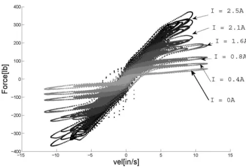
(20) Introduction. 5. Figure 1.4: Behavior of the damper using different excitation current inputs.. and the output damping force of the M R shock absorber. It is based on a Linear Parameter-Varying (LPV) system, which is proposed to allocate the non-linearities and hysteresis ofthis device. Because of the fact that the L P V model will reproduce the M R damper's behavior in a single structure and based on a dynamical system, it is proposed to obtain better output results than the state of the art schemes studied. This will be later proved by comparing statistical indexes of model errors between the models analyzed. Due to the combination of being single-structured and have good accuracy, this model might later be used for control, observation or simulation purposes. In order to better understand the main characteristics of the model to be developed, a brief introduction to L P V systems is shown below.. 1.3.1. Linear Parameter-Varying Systems. Linear Parameter-Varying (LPV) models belong to the set of Linear Time-Varying Systems. These systems have finite dimensions and its state-space representation is given by the weighted sum of local state vectors. In this way the dependency on time is hidden among its parameters. Equation (1.1) shows the expression of a generalized L P V system, taking the form of a non-autonomous and non-stationary system of linear differential equations with vectorial equalities.. (1.1). are the states, the exogenous input and measured output of the system, respectively. Parameter p(t) acts internally in the model to modify the behavior of the system, it is delimited on a finite space, as shown in equation (1.2), where the relationship is valid only i f U is bounded. p.

(21) 6. The importance of this model, resides in the ability to modify its dynamics over the time, which makes it proper to model non-linear and time-variant systems, such as the M R damper. It will be shown the importance of the "pointer" variable (p) which changes the states according to a variable of scheduling, whose selection, will be essential for the correct modeling of the shock absorber. Furthermore, this L P V model analysis can be combined with control design techniques using p, H. T O. and H. 2. norms, loop shaping, and others, to generate control schemes allowing robust and performance specifications.. 1.4. Thesis objective. The main objective of this thesis is to develop an experimental L P V model for the M R damper, in order to emulate the behavior of the shock absorber, and analyze its results comparing its performance with other state of the art models. In order to do so, a set of experiments with the M R damper will be performed, introducing excitation signals to the shock absorber, and measuring the response of the damper under these conditions. The excitation signals will be representative of the different operative conditions under which the damper could be subjected. The models will be learned by using this data, allowing to obtain real simulators of the damper, and based on the comparison in the performance of them, it will be concluded if the L P V system is a more suitable model for the damper, than the conventional models defined afore.. 1.5. Outline. This thesis is organized as follows: a more complete state of the art review is shown in Chapter 2, and the proposed L P V model structure is shown in Chapter 3. In Chapter 4 the design of experiments (DoE) and the experimental setup for the M R damper is explained. The modeling results are shown in Chapter 5, while a discussion of these results will be found in Chapter 6. Finally, the conclusions of this research will be discussed in Chapter 7..

(22) Chapter 2. MR Damper Models Review 2.1. Introduction. In this Chapter, an analysis of the state-of-the-art models is realized. A model is a mathematical structure that permits to replicate the dynamic behavior of the M R damper, and by the use of them, it is possible to measure the physical capabilities and limitations ofthe damper. The challenging problem with the modeling of the damper, resides in the non-linearities and hysteresis that the damper contains. Depending on the nature of the model, it might be possible to find, in the state of the art, model structures based on a physical principle of dynamics, a pure mathematical architecture, or even a black-box structure, where the contents of the model are unknown. However the model, it is impossible to cover neatly the M R damper conduct, due to the high complexity of its nature. A n optimization tool will be required in order to learn the models, based on the real data obtained from the experiments (see Chapter 4). Different Model architectures are reviewed below. Among the existing architectures, the structures classified as Black-box, Phenomenological, and Semi-Phenomenological will be the main categories of models focused on this research. These architectures have been chosen because they have been previously analyzed in the field of modeling of M R dampers, and might be suitable for applications of control design.. 2.2 2.2.1. State-of-the-art review Semi-Phenomenological models. A Semi-Phenomenological (SP) model describes the dynamics of a process using a mathematical relationship partly based on the conduct of a physical phenomenon. The numerical value of a coefficient may refer to a physical dimension whose real meaning exists. The result is a model based on a combination of an analysis of physical characteristics of the system, and mathematical techniques to aid the representation of them. Two SP structures are described in this section: the first one was proposed by [Guo et al., 2006] and contains a model based in the description of the hysteresis by means of an hyperbolic function; the second one, proposed by [Spencer et al., 1996], is similar to the first structure but it uses a coupled non-linear equation in order to enable it to emulate hysteretic systems.. 7.

(23) 8. Semi-Phenomenological model 1 One of the models that can be considered in this category was proposed by [Guo et al., 2006]. This model uses the velocity to describe the hysteretic behavior of the damping force. It is defined by the equation ((2.1)). (2.1) where F. (t) is the damper force, x(t) refers to the position of the damper piston, and v(t) is the velocity of the. mr. damper. V and X are respectively, the absolute values of hysteretic critical velocity and displacement; those are 0. 0. also the piston velocity and position where the F fluid. Parameters A and A 2. 3. m. r. is zero. A\ is defined as the dynamic yield force of the M R. are related to post-yield and pre-yield viscous damping coefficients, respectively.. Figures 2.1 and 2.2 taken from [Guo et al., 2006] show respectively the shape of the force-velocity curve produced with this model, and a graphical representation of the model.. Figure 2.1: The schematic of the SP model, where k\ [Guo et al., 2006]. From Figure 2.2, it can be seen that the sign change of the variables force and velocity is similar, always with a delay from the force signal. This also happens with the force-velocity signals produced during operation of the damper. This is an important characteristic of the hysteretic behavior referred previously.. Figure 2.2: Shape of the curve produced by the SP model, taken from [Guo et al., 2006]..

(24) 9. MR Damper Models Review. Semi-Phenomenological model 2 Other model that can be classified within this group, is the model proposed by [Spencer et al., 1996], which is based on the Bouc-Wen model, and it is shown in equation (2.2). It is a second-order linear model, with an integrated non-linear equation, which gives the ability to emulate hysteretic systems.. (2.2) A way to interpret this model, is shown in Figure (2.3), taken from [Spencer et al., 1996]. It contains an arrangement of mechanical impedances that reflects the physical behavior of the model. This model is characterized by 10 parameters; z(t) changes over time, depending on the rate of change of position variables x(t) and y(t). Parameter n is a positive integer, and according to [Savaresi et al., 2005], it's best value was found to be 2.. 2.2.2. Black-Box Modeling. A Black-Box model can be viewed most of the times as a system whose internal workings are not important, unknown, or are based on a predefined structure. It may just be seen as a block (black-box) with inputs and outputs that represents the dynamic behavior of a system. These models are widely used to reproduce systems with no a priori information available such as stochastic processes, financial behaviors, and as in this case, non-linear processes. Structures suitable for this type of modeling are neuronal networks and recurrence equations (ARX, N A R X , A R M A , N A R M A , A R M A X , N A R M A X ) [Savaresi et al., 2005] [Jin et al., 2005] [Nino-Juarez et al., 2008]. Examples of these models are briefly reviewed in this section. NARX model In [Savaresi et al., 2005] a Nonlinear AutoRegressive Exogenous model (NARX) for a M R damper was proposed. It is shown in equation (2.3) where F. m r. , x and v are the force, position and velocity of the damper respectively.. Figure 2.3: Physical representation of the modified Bouc-Wen phenomenological model, taken from [Spencer et al., 1996]..

(25) 10. (2.3) Coefficients a are to be found by training the model with experimental data. It was concluded that this number of regressors (2,2,2) was the best choice to capture the damper dynamics. Force and velocity signals were found to be particulary important for the performance of the model; when this two signals were used, good performance results were found, even i f the position regressors were not included. Force regressors were observed to be essential to obtain a good model, without them, no good results were met. In [Nino-Juarez et al., 2008] a black-box model with a similar structure was used. It contained the same variables as inputs (force, position and velocity), but with a different number of regressors (3,3,3). A recursive least squares algorithm was used to perform the learning of the parameters from real data. A performance analysis was done, when the model was trained using different input frequencies.. 2.2.3. Phenomenological Modeling. A Phenomenological model can be used to describe a the dynamics of a physical system, obtained from empirical observations of a phenomenon, so that is consistent with physical theory but not directly derived from it. Phenomenological models differ from structured models because they only partially reflect the actual physical structure of the system. Some of these models have been used in previous works [Spencer et al., 1996] [Burton et al., 1996] to replicate the M R damper dynamics. The Bouc-Wen model can also be classified in this field. The main difference between these models and the semi-phenomenological structures seen in section 2.2.1 is that part of the mathematical description of SP models contains a physical meaning, and might be related to a real entity; in the Phenomenological models it is not possible to find a clear relationship between the mathematical description and the physical arrangement of the system. Two Phenomenological models are studied in this section: the first one was proposed by [Wang and Kamath, 2006], and is based in a physical analysis of the change of state on the smart material of the M R damper; the second one was proposed by [Kwok et al., 2006], based on the Bouc-Wen model, uses an evolutive variable to describe the M R damper hysteresis by means of a hyperbolic function. These models are fully described below. Phenomenological model 1 In [Wang and Kamath, 2006] a phenomenological model was proposed. It is based in the mathematical description of the evolution of the shear stress of the material inside the M R damper, when it changes from a solid state to a semi-solid as described in Figure (2.4), taken from [Wang and Kamath, 2006]. To construct this relationship a lagrangian analysis was performed, using the constitutive mechanical relationship between the magnitudes of stress and deformation of the material, and defining the kinetic and potential contributions for the phase transition, and finally associating this model with the real output and input signals of the M R damper. This is described in equation (2.4). (2.4) It is a second-order nonlinear ordinary equation, where v(t) is the input velocity of the shock absorber and F. m. r. (t) is the damper force. Parameters F. m. r. (t),. r. (t), and. r. (t) are used in the equation to represent the hys-. teresis of the M R damper, by recreating the phase transition of the M R fluid in the one-dimension case. Parameters F. m r. (t) and F. m. r. (t) in the model, are used to capture the dynamics of the phase switching in the M R damper..

(26) MR. DamperModelsReview. 11. Figure 2.4: Three phases of Magneto-Rheological fluids under shear stress loading, taken from [Wang and Kamath, 2006]. According [Wang and Kamath, 2006], in order to replicate the M R damper behavior all coefficients (wj) should be identified using experimental results. These coefficients must be assumed dependent on the magnetic field to achieve a more general model. The dependency can be approximated by a polynomial and should be identified from experimental data too. Phenomenological model 2 In [Kwok et al., 2006] a phenomenological model was presented. This model, based in the work of Bouc-Wen [Spencer et al., 1996], pretends to represent the hysteretic behavior of the M R damper, by the use of an evolutive variable, that changes according the velocity and its position respect the asymptotic natural stable position of the damper, as shown in the arrangement of Figure 2.5. This model is shown in equation (2.5).. Figure 2.5: Physical representation of kwok proposed model, taken from [Kwok et al., 2006].. (2.5) where k is the scale factor for the modeled hysteresis, k and k are the viscous and stiffness coefficients re3. 1. 2. spectively, k is the damper force offset, and z(t) is the evolutive variable, which emulates the hysteretic conduct 4. aforementioned, by using a simple hyperbolic tangent function, which enhances its performance in the criterion of parameter identification and computation efficiency. In order to make the model current dependant, coefficients might be made equal to a linear time function of the applied current, according to [Kwok et al., 2006]..

(27) 12. 2.2.4. Model summary. In order to better appreciate the differences between the systems analyzed, Table 2.1 shows a brief summary of the model characteristics reviewed in this Chapter.. Table 2.1: Model characteristics summary.. Based on the amount of parameters, the most complex model is the one of [Spencer et al., 1996], which has a dynamical structure with an embedded differential equation in the model. Models [Guo et al., 2006], and [Wang and Kamath, 2006] contain only five parameters, thus representing a relatively simple structure. Models [Kwok et al., 2006] and [Guo et al., 2006] contain an static relationship between input and output variables, as they do not take into account historical data of the signals involved. This might be convenientfor models seeking simplicity, but these systems might loose some accuracy when doing analysis like frequency response or control synthesis. Embedded evolutive variables increase the complexity of models, however, they allow represent hysteretic be¬ haviors in the damper. Nonetheless, this conduct might also be replicated by single-structured models, as in [Guo et al., 2006] comparing this point will be important to evaluate the performance of these models. It is also possible to appreciate that none of the models studied include the current dependency on its structure. This important feature is vital to obtain a more complete representation of the M R damper. Even i f the model can replicate the hysteresis of the system, when modifying the current level on the damper's coil, the model will have to adapt its parameters in order to suit the new behavior of the shock absorber. If the model does not include the current dependency, it might not be able to replicate the M R damper behavior in a complete manner. It is possible though, to insert the current dependency by making the coefficients dependent on the current, which might at the same time increase the model complexity. If the model contains both the hysteresis and non-linear characteristics of the M R damper, it is also possible to identify if there is a dependency between these two components that can influence the output model force. The L P V proposed model will contain the above necessary and desirable characteristics to extensively reproduce the M R damper conduct with a goodperformance: reproduce dynamically (historic-based) the M R damper behavior; nest both the hysteresis and non-linearities (current dependency) characteristics of the shock absorber; and contain the aforementioned characteristics in a single-structured model. The model L P V that is proposed will not contain single parameters, but a set of matrices which will build a dynamical system, associating the velocity and current to the output force of the M R damper. By means of this structure, it will be possible to design a control scheme for the M R damper, or the quarter of vehicle system. L P V model structure will be fully described in Chapter 3..

(28) Chapter 3. LPV Model Formulation. 3.1. Introduction. The objective of this Chapter is to demonstrate that it is possible to create an L P V model for a M R damper. Several model structures have been proposed in order to solve the problem of replicating the M R damper non-linearities. However, in order to do this, some of them rely on static relationships between the force and its excitation inputs, which might not take into account some important dynamical features of this device. Others, depend on factors that might well reproduce the M R damper force, but only under certain conditions (a certain current level, for example), and in order to boost its capacity to all working conditions, additional coefficients shall be added which complicates its initial simple structure. In [Poussot-Vassal et al., 2008], [Lozoya-Santos et al., 2010], and [Anh-LamDo, 2010] an L P V structure was used to represent the quarter of car model, which embodies the devices shown in Figure 1.3. These models use either the changing mass value of the suspension or the M R damper force as an scheduling parameter in order to adequate the model to the working conditions of the suspension system. Based on these models, a robust control strategy was designed for each structure, in order to regulate the vibrations applied on the suspension. The L P V model proposed in this thesis will only describe the behavior of the MR damper shown in Figure 1.3. It will recreate the relationship between the displacement velocity and the electric current with the damper force, in a single structure. This new model represents an innovative way to reproduce the M R damper behavior, using an structure com¬ pletely different as the ones reviewed in Chapter 2, but taking into account all the features of the system that have to be considered to provide an extensive model of the damper. The proposed structure is designed using an L P V polynomial system as described in [Bamieh and Giarre, 2002], parting from a discrete-time system and a piecewise variable, to recreate the hysteretic behavior of the M R damper, that depends on the input velocity and electric current. A n extended model of the quarter of car system might later be produced using the proposed system in order to design a control strategy of the whole suspension, similar as in [Lozoya-Santos et al., 2010], and [Anh-Lam Do, 2010].. 3.2. Linear Parameter-Varying (LPV) systems. Linear Parameter-Varying (LPV) systems belong to the set of Linear Time-Varying Systems. These systems have finite dimensions and its state-space representation is given by the weighted sum of local state vectors. The de-. 13.

(29) 14. pendency on time is hidden among its parameters.. A L P V system can be viewed as a combination of Linear. Time-Invariant systems (LTI) and in some cases as a Linear Differential Inclusion (LDI). Equation (3.1) shows the expression of a generalized L P V system, taking the form of a non-autonomous and non-stationary system of linear differential equations with vectorial equalities.. (3.1) where x ( t ) G X c |. n. x. n. , u(t) G U c l. m. and f (t) G F c I. s. are the states, external input(s) and measured. output(s) of the system, respectively, n is the system's degree, m is the number of the inputs, and s is the number of outputs of the system. Parameter p(t) acts internally in the model to modify the behavior of the system, it is delimited on a finite space, as shown in equation (3.2).. (3.2) where the relationship is valid only if U is bounded and k is the number of scheduling parameters of the L P V p. model. The importance of this model resides in the ability to modify its dynamics over the time, which it makes proper to model non-linear and time-variant systems, such as the M R damper. It will be shown the important use of the pointer variable (p(t)) which changes the states according to a variable of scheduling, whose selection, it will be essential for the correct modeling of the shock absorber.. 3.2.1. Internal parameters. Linear Parameter-Varying systems performance strongly depends of parameter p(t) that acts internally in the model to modify its dynamical behavior. However, this parameter might be defined in different ways inside the model, according of the nature of the system to model. In general, this parameter might be sorted into three main groups: 1. Parameter as a function of state. Scheduling parameter could be dependant of a state variable of the system. By definition, the internal parameter of the L P V model (p) has to be bounded in a finite space, while the state variable can achieve infinite values, although generally for most applications, it is not true (state variables lie within a finite space). For this, when a L P V system uses states in the parameters expressions it is called a Quasi-LPV system. 2. Internal Parameter. These parameters are usually found when modeling time-variant systems. The parameter is in this case, an interior expression of the model, regularly involving non-linear terms. States change accord¬ ing to this expression, such that the information used to compute the parameter is dependant of the system internal dynamics and elapsed time. 3. External Parameter. The parameter that changes the model dynamics, has to be an external variable, nondependent on the system, and whose variations changes the system behavior. As can be thought, this type of models are suited to be used for control and observer purposes. This type ofparameter will be used for the case of study analyzed in this work..

(30) LPV Model Formulation.. 3.3. 15. LPV model structure. The L P V system's morphology is given by a combination of Linear Time-Invariant (LTI) models, governed by an scheduling variable, subjected to the working conditions of the system. For the case of study, the scheduling variable is an external parameter, non-dependent on the system, and will be defined in section 3.5. This external parameter will be linked to the system by the use of a polynomial relationship, based in [Bamieh and Giarre, 2002]. The proposed model structure, for the time-continuous case was shown in Equation (3.1). Matrices dependency to the scheduling variable are proposed to be achieved by means of a polynomial linear system, as shown in Equation (3.3), based in the work of [Bamieh and Giarre, 2002].. (3.3). (3.4) where p. m i n. , and p. m a x. are the lower and upper values of the scheduling parameter. It is important, when using such. type of formulation, to ensure that the system defined by p-dependent matrices is stable within its defined region, this because it will be required for the control design formulation, and in order to maintain the system stability when using the model as simulator of the M R damper. This property will be guaranteed for the case of the M R damper in section 3.6. According to the LPV-structure defined previously it was assumed that the non-linearities of the device modeled, can be approximated to an state space model, with matrix coefficients defined with a polynomial equation. This assumption will be later used in the model formulation, in order to denote the scheduling dependency of the L P V structure.. 3.4. Discrete-time LPV model definition. Non-linear approximation of equation (3.3), can be referred to the case when the model is defined using a discretetime transfer function. Here the extensive model can be defined as in equation (3.5). (3.5) where, the numerator N(z,p) and denominator D(z,p) are dependent on the z-discrete operator and scheduling pa¬ rameter p. They can be defined as:. (3.6). where n is the degree of the discrete version of the system. Using a similar assumption as in equation (3.3), it is considered that the non-linear approximation of the system modeled can be achieved making the coefficients of the transfer function a polynomial equation dependent on the scheduling parameter; this way the coefficients can be computed as:.

(31) 16. (3.7). where Np is the polynomial degree of the non-linear approximation. Whentransferring this discrete functionto the state space framework(see Appendix A), for the case o f a model in a controllable canonical structure, the latter will become:. (3.8). and the output:. (3.9). Which clearly agrees with the L P V system's structure defined in equation (3.3). Applying scheduling-dependency of equation (3.6), model matrices from equation (3.8) canbe computed as:. (3.10). (3.11). And the output matrices C(p(t)) and D(p(t)), of equation (3.9) can be computed, when assuming b (p) = 0, as 0. follows:. (3.12).

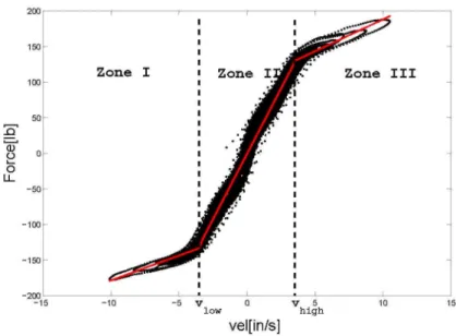
(32) LPV Model Formulation.. 17. (3.13) D(p(t)) = 0. (3.13). This last assumption can be done, due to the fact that the system behavior does not show an instantaneous response when a displacement excitation occurs, D(p(t)) = b = 0. 0. 3.5. Scheduling parameter. Scheduling parameter is of great importance in the L P V model formulation, its correct selection is vital for the system's performance, and correct cohesion with the desired dynamic representation. For the case of study, M R damper's non-linearities are greatly related to the input current level of the coil. This relationship can be clearly appreciated in Figure 3.1, where the damper force-velocity static plane is shown for the case of different current levels.. Figure 3.1: Behavior of the damper for different current-static levels of excitation. A more clearly dependency can be appreciated, when looking at Figure 3.2, where it is shown an static forcevelocity map of the M R damper, and a regression made using the piecewise straight-line equation (3. 14).. (3.14). For each of the three zones seen in the plot, a m -slope and c -intercept of a linear equation was calculated. 4. This analysis was made for different current values and the results are plotted in Figure 3.3. A clear influence of the current can be appreciated in the straight line slopes, as the current grows up, the slopes also becomes larger. In order to interpret this clear relationship, the scheduling parameter will be designed as the input current level.. (3.15).

(33) 18. Figure 3.2: Measured and straight-line regression force-velocity graph, @1.2 Amps.. Figure 3.3: Force-velocity identified slopes and intercepts for straight-line regression for all electric current levels..

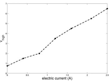
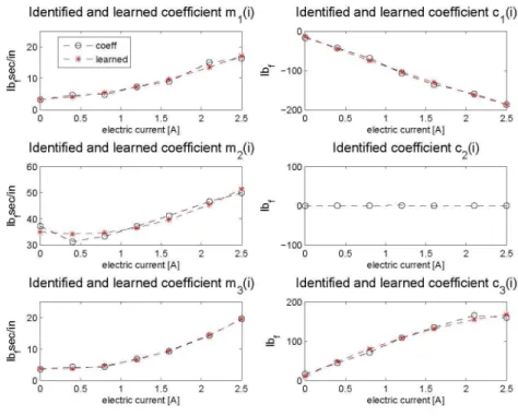
(34) LPV Model Formulation.. 3.5.1. 19. Input signal and hysteresis replication.. Due to the complex dynamic behavior of the damper it is important to complement the non-linear model formulation by analyzing the relationship between the excitation signals measured or calculated in the experiments and the output desired force signal. It is possible to appreciate in Figure 3.1 that the output force of the M R damper is clearly related to the displacement velocity of the damper and the electric current level of the system. However, as it can be seen in Figure 3.4, when modeling the M R damper with an LTI system using solely the displacement velocity signal as the input variable and the M R damper force as the output signal, it is impossible the replicate the damper behavior when it explores the hysteretic zones in the force-velocity static plane.. Figure 3.4: Model output results when modeling the M R damper using an LTI system. Experiment 8 (1.2 Amp). As seen in Figure 3.2, it is clear that the force-velocity relation changes when the velocity surpasses or fall behind certain velocity limit. These limits are symmetric ( v. h i g h. = -v. I o w. ) , and they can be found by inspection in. the force-velocity graph. These limits also change with the input current level, as it can be seen in Figure 3.5. Velocity limits show a very linear behavior with the electric current, and will be fitted to a first order algebraic equation in order to shape this relationship, as seen in equation (3. 16).. (3.16) this way the velocity zone where the damper is situated can be monitored for constant or persistent electric current patterns. The importance of these limits resides in the fact that the input variable ought to contain also a different behavior when the velocity changes from zone to zone in the force-velocity map. Input variable definition A new input variable will be computed based on the above observations, such as it detects when the damper is exploring an hysteretic region, and takes into account the force-velocity change to aid the L P V model to remain attached to the M R damper force..

(35) 20. Figure 3.5: Behavior of the v. high. limits for different electric current levels.. The relationship between the input variable u(t) and the velocity v(t) is proposed to be a simple scalar formula, generated by an algebraic relationship shown in equation (3. 17).. (3.17). where variable <r(i(£)) is a scale factor of the velocity, used to aid the L P V model to follow the hysteretic shape of the force-velocity static plane, and it will reduce the velocity magnitude when it surpasses its border limit defined previously. Variable ^(i(t)) is just a correction factor to ensure variable continuity near in the scale changes. It is:. (3.18) Scale factor a(i(t)) and correction factor ^(i(t)) are computed using the data from analysis seen in section 3.5. They will be computed using a simple normalization of the m-slope and c-intercept coefficients of the force-velocity static relationship, with the central slope m ( i ( t ) ) , which is always the biggest slope value. 2. (3.19). (3.20). where m (i(t)), m (i(t)), and m (i(t)) are the force-velocity magnitude relationship for zones I, II, and III, and i. 2. 3. c (i(t)), c (i(t)), and c (i(t)) are the offset coefficients for the same zones. i. 2. 3. The normalization by the parameter m2(i(t)) is done in order to maintain the force-velocity relationship un¬ touched when using the same LTI model to represent three different zones of the force-velocity static plane..

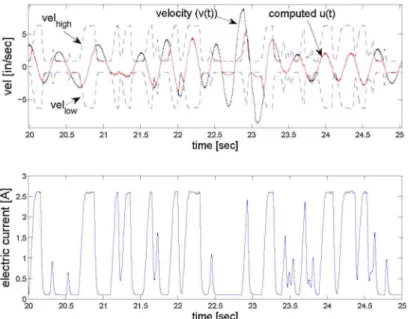
(36) LPV. ModelFormulation.. 21. coefficients, and the fitting of these equations is shown in Figure 3.6, where coefficient c is not identified for its 2. low neglectful value.. Figure 3.6: Identified and fitted curves of coefficient equations. It is possible to appreciate the symmetry of the identified coefficients. For the zone I and zone III, learned slopes are very similar, and the constant values of the curve have magnitudes akin, but with different signs. For the case of zone 2, the magnitude of the slope is always greater than in the other zones as was expected, and the constant value contains a marginal value, which will be neglected. Summarizing, the input variable that will aid the L P V model to follow hysteretic patterns, can now be computed as shown in equation (3.21).. (3.21). To demonstrate graphically the function of this variable, equation 3.21 is now used to compute u(t) for the case of a displacement pattern with constant current. The results are shown in Figure 3.7, where the scale factor is clearly applied when the velocity surpasses the limit allowed for that electric current value. This scale factor will permit variable u(t) behave differently in the three different zones. For the case of a persistent current experiment of Figure 3.8, results are similar, but in this case, velocity limits changes in time, increasing the complexity of the analysis. However, as it can be seen, the scaled variable keep.

(37) 22. Figure 3.7: Above, velocity v(t) and computed input variable u(t); below, constant electric current applied to the experiment 8 (0.8 Amp).. changing in a very similar way as the velocity.. Figure 3.8: Above, velocity v(t) and computed input variable u(t) for experimental test 2; below, persistent electric current applied to the damper..

(38) LPV. ModelFormulation.. 23. Figure 3.9: Root locus analysis of the L P V model, under incrementing current values in the input coil.. 3.6. Stability analysis. In order to ensure the stability of the M R damper model, an analysis of stability was done. This study is based on the learned matrices of the L P V model, shown in Appendix C. From these matrices, it is possible to plot a root locus analysis, and assure that this model will be stable for all the working zones of the damper. Using state space matrices A. 0. and A. i. (see Appendix C), the eigenvalues of the system were calculated for. different electric current values, in the range of i G [0 , 2.5]A, which it is the operating range of the system. It was found that the eigenvalues of the system behave as shown in Figure 3.9, where the arrows indicate the direction where the poles are moving while the electric current is being incremented. The diagram shows a discrete-time root locus analysis of the system, with the original values of the eigenvalues (with an electric current of zero), denoted by the arrows. The pole 1 remains static (a. i. = 0.83) while the current. grows; pole 2 approaches the unity value with an initial negative value, but it never reaches it. Poles 2 and 3 have conjugated complex values that follow the path described by the arrows in the central part of the graphic, as it can be seen, they always have an absolute value lower than one. It is clear that the eigenvalues do not surpass the unity circle, for the electric current range evaluated. In fact, it would be necessary a current of 9 A in order to make the model unstable, a value unreachable in the M R damper coil. This analysis ensures that the proposed L P V system will be stable, when working under the nominal operating conditions..

(39) 24. 3.7. LPV model summary. The general structure of the proposed L P V model in this Chapter is resumed in the model diagram of Figure 3.10.. Figure 3.10: Proposed L P V model structure. where scale function u(v(t),i(t)) is a piecewise function computed as follows:. (3.22). (3.23). with P(t) = i(t) For the case of the model found in this work, these matrices were only made equal to a first order polynomial equation. A more detailed summary of this modeling procedure is included in Appendix C..

(40) Chapter 4. Design of Experiments 4.1. Introduction. The research objective of this work is related to the identification of a dynamical system. The information used to compute the model that will replicate this device's behavior will be obtained from real data measurements, generated from experimental tests. In order to do so, a set of experimental essays was designed, defining different excitation patterns for the most important input variables of the M R damper [Lozoya-Santos et al., 2009a]. In order to accomplish the tests, a mechanical setup with the M R damper was implemented, including measure¬ ment devices, electric current patterns controls and displacement actuators that will be later described.. 4.2. Experimental Setup. A set of displacement and current excitation signals will be applied into the M R damper. To accomplish the me¬ chanical tests over the M R damper, an experimental setup was done. The M R damper analyzed in this test is part of TM. 1. a Delphi MagneRide suspension system, as seen in Figure 4.1 .. DCLPHI. 1. Figure 4.1: M R Damper device used in the tests . The experimental setup contains three principal components: Actuators (displacement and current), data acqui-. 25.

(41) 26. sition (DAQ) devices, and a control system. Actuator system receives commands from de control system, which injects the excitation patterns into the M R damper. The data acquisition system, measures the system response under these excitation signals. TM. A n MTS controller GT testing system was used to control the position of the damper, as shown in Fig. 4.2, TM. taken from [Lozoya-Santos et al., 2009b]. A data acquisition system Flextest commanded the controller and recorded the position and force from the M R damper. A sampling frequency of 512 hertz was used. The experimental setup was controlled and monitored from an interface developed under the LabView. TM. framework.. Figure 4.2: Experimental setup block diagram. Hydraulic servo-controlled piston introduces a displacement excitation pattern ( x ) commanded by the D A Q system i n. and measured in the L V D T sensor ( x ) . M R damper force (FMR) is measured by m s. means of a load cell located at the union of the damper and the piston. Electric current excitation is introduced into the damper, and is measured by a electric current transducer. Measured signals are directed to the D A Q system, and monitored in the H M I .. M R damper displacement is guided by a hydraulic servo-controlled piston actuator of 3,000 psi of capacity and displacement bandwidth of 15 Hz, which lies within normal automotive applications. Electric excitation is put into the damper coil using a P W M current driver and the output signal is measured by a current sensor and directed to the signal data acquisition system. Force signal is measured using a load cell in the piston-damper connection, this device contains an stress gauge to measure the force and an accelerometer to neglect its own mass. Position is measured using a Linear Variable Differential Transformer (LVDT), allocated into the piston. The displacement and electric current range were: 0 - 0.04 m, and 0 - 4 A respectively. The measured span of the M R damping force was 0 - 2850 N ..

(42) 27. Design of Experiments. 4.3. Design of Experiments (DoE). The objective of the experimentation is to extract the M R damper dynamical response by obtaining data of the damper under representative working conditions with a proper frequency content. To do this a set of generate displacement and electric current input patterns where designed. These patterns will be chosen so that they can also aid the modeling process of the system. Eight test were defined in order to do the aforementioned process. They contain a set of displacement and electric current patterns that meet the specification described above, and that that will produce the M R damper appropriate response to aid the fitting process of mathematical modeling. The amount of experiments was determined based on the amount of excitation patterns defined in the DoE, and the possible combination produced by this means. For each experiment, ten replicates were produced in order to find statistical validity to the results. The aforementioned patterns are described below.. 4.3.1. Electric current patterns. Electric current patterns are very important for the system identification. The correct selection of these signals must take into account the settling time of the electric circuit involved in the coil, the electric current input limits of the M R damper, and the signal reachability of the experimental setup (described later in this Chapter). The electric current patterns used for the experimental tests are shown below. Increased Clock Period Signal (ICPS) This signal modifies the signal amplitude randomly every constant period of time. The time period must be bigger than the stabilization time of the M R damper. Because of its random content, this signal is rich in frequency, an important factor for system identification. As seen in [Soderstrom and Stoica, 1989], the ICPS signal can be computed as shown in equation (4.1).. (4.1) where. is a uniformly distributed noise signal, N. 1. C. P. S. is the number of sampling periods over which the signal. amplitude is held constant, and |_sj represents the integer part of s. The fact that the signal holds the value of the current over a specific period of time allows the design to con¬ template the settling time of the transient part of the dynamic response of the damper. For the case of study, the signal content of the current was defined to be bounded between 0 and 2.5 A , with a changing period of 20 ms. The sampling frequency was defined as 512 Hz. Pseudo-Random Binary Signal (PRBS) Generates a signal rich in frequency, whose amplitude changes between two values, with a pseudo-random period of time (defined by a binary sequence). The time duration of every step is governed by a binary algorithm using a shift register whose length depends on the settling time of the system to identify, in this case, the M R damper. Appendix ?? contains a more complete description of the signal generator used for this sequence. The signal is defined between the boundary values of the current 0 and 2.5 A . The number of cells in the shift register was chosen such that the settling time of the system can be achieved in the transient response of the damper, defined as 20 ms. The sampling period used in this signal was 1/512 sec..

(43) 28. Amplitude Pseudo-Random Binary Signal (APRBS) This signal produces a pattern similar to the PRBS signal, but instead of changing between two constant values, every pseudo-random period of time, the algorithm also changes randomly the signal value by means of a uniformly distributed noise signal. This signal was defined because in normal operation the damper will probably not change only between two current values, and this has to be embodied in the pattern. It was also meant to increment the frequency content of the signal. The distribution function of noise used to calculate this signal was defined between 0 and 2.5 A , with a settling time defined as 20 ms, and a sampling frequency of 512 Hz. Stepped Increments Signal (SC) This signal produces a pattern with constant electric current values, changed every predetermined period of time, usually much longer in comparison with the settling time of the system. At the end of this time period, the signal value is incremented a certain amount of current. This is one of the most used signal pattern [Spencer et al., 1996] [Guo et al., 2006] [Nino-Juarez et al., 2008] [Wang and Kamath, 2006], and is defined in this way in order to evaluate the system response in each current value, and extract a more complete information of the damper conduct. This signal is also easy to achieve for it might no need a sophisticated hardware to control the coil of the damper. Using this pattern is also possible to find a linear tangent approximation of the damper's behavior by contem¬ plating each current value as a linearizable point of the model. There were 7 values of current used in this pattern (0, 0.44, 0.8, 1.2, 1.6, 2.1, and 2.5). The time at which the current value changes, depends on the duration of the displacement pattern, which was of 30s for most cases.. 4.3.2. Displacement Pattern. Different displacement patterns has been defined in past works in order to produce a displacement excitation in the damper. As stated in [Wong, 2001] signals such as sinusoidal or triangular waves, and stepped patterns are commonly used as displacement profiles for the damper testing. However, these patterns don't recreate a pattern simulating a natural response of the damper under operational conditions. A Road Profile (RP) pattern is a signal that recreates the conduct of an specific type of road, in this case of a highway under normal operational conditions and contains a displacement wave time-changing in frequency and in amplitude. This type of pattern was chosen to do the testing of the M R damper due to its representability of working conditions under nominal operation of the suspension. It is important, in order to recreate this pattern to define the road which is the signal is defined. As can be expected it is possible to describe each road according to the frequency content of the signal produced. According to standard ISO 8606:1995, there exist eight different types of roads depending on the power spectral density. This coefficient is computed, as stated in [Wong, 2001] as shown in Equation 4.2.. (4.2) where S ( f ) is the power spectral density of the elevation of the surface profile, v is the speed of the vehicle, f is c. the signal frequency in Hz, UJ is the number of cycles per feet, C is the road roughness coefficient, and N X. r. roughness coefficient of the road. Table 4.1 shows the C and N r. of roads, obtained from [Wong, 2001].. c r. c r. is the. roughness coefficient values for different types.

(44) Design ofExperiments. 29. Table 4.1: Roughness coefficients in power spectral density function.. Road profile pattern can be computed by a sum of harmonic waves, which will produce the sinusoidal pattern described above. The displacement pattern equation is defined in equation (4.3). (4.3) where x. r o a d. ( t ) is the displacement of the road, 4>j is a random phase angle defined with a normal distribution. between 0 and 2n. ujj is a frequency within 0 and S ( f ) and calculated as: (4.4) where A w is the frequency increment computed as A w = ( w increments in the interval w. m i n. - w. m a x. m a x. - w. m i n. ) / N f ; Nf is the total number of frequency. , which are the minimum and maximum frequencies of the pattern.. The signal magnitude will be continuously changing and is governed by the squared-root term. The bigger the value of the power spectral density, the bigger the magnitude of the signal obtained. For the case of study, the chosen type of road was of a smooth highway, with a vehicle under a speed of 440 in/s (25 mi/h). The number of harmonics was set to 100 with a frequency span defined between 0.5 and 20.5 Hz. The number of cycles per feet was chosen as 0.5. The obtained signal reaches displacement values of 0.5 in, and frequency peaks values of around 6 H z. 4.4. Experiments content. Eight pairs of current-displacement training patterns were selected to obtain the data for the modeling of the research of the present work. The content of these tests is shown in Table 4.2. The first five training patterns contain recurrent signals (changing in time) for the electric current pattern. These tests were performed in order to obtain experimental data of the M R damper recreating the working conditions of the damper, with richer frequency content of the signals. These test will represent an useful data base for the training of electric current dependent models, and for the validation of the results obtained during the learning process of the system. Experiments 6-8 contain SC (Stepped increments) in the electric current pattern of the tests. This type of experiment has been used in [Spencer et al., 1996] [Nino-Juarez et al., 2008] to produce a tangent linearization of the system in different local zones of the electric current map. By using these experiments it will be possible to generate an important analysis related to the L P V model definition, seen in section 3.5. The electric current peak value for all experiments is of 2.5 Amperes. Experiments lengths are different, most of them have a duration of 30 seconds, but some of the tests have a duration of 600 seconds (20 times the normal length). While tests are performed, thermic remanent of the coil.

(45) 30. produces an increment of the temperature of the damper. Long-time experiments might be used to analyze i f the M R damper behaves differently under contrasting thermic conditions. For each training pattern, various replicates were done. These replicates were made to give validation data for the models. Eleven replicates were done for tests 1-3, which represents 330 seconds of data, an amount of time enough to show contrasting conditions in temperature over the damper. For experiments 4 and 5, a total of 3 and 4 replicates were done respectively, containing the longest amount of data of the experimental data base produced (1800-2400 seconds, 30-40 minutes). Finally, for experiments 6-8 a total of 7 replicates were performed, each of them with a different electric current static value, separate enough from each other to differentiate the contrasting zones of the electric current map.. Table 4.2: Experimental tests content in Design of Experiments (DoE).. The signal content of one of the experiments (experiment 1) is shown below. It is possible to see the current and displacement excitation pattern, and the frequency content of this last signal excitation over the time. The complete review of the signal content of each experiment is shown in Appendix D.. 4.4.1. Experiment 1.. Figure 4.3: Displacement and current signals (left), and displacement frequency content (right) of experiment 1..

(46) Design ofExperiments. 31. 4.5. Signal conditioning.. 4.5.1. Noise filter. Measured data contained unavoidable noise signals, that were removed from the displacement patterns. As it cab be seen, the filter designed to remove this noise was a second order low-pass filter with a cutoff frequency of 20 Hz, as shown in equation (4.5). The discretization method to obtain the filter was by supposing an input Zero Order Holder (ZOH) in the system, and a time period of 1.953 msec (512 Hz). Figure 4.4 shows the frequency response of this filter, where it is clear that the frequency cutoff corresponds to a 40n rad/sec (20 Hz.), frequency above the displacement signals corrected. Figure 4.5 shows an example of the signal treatment done by this discrete-filter.. (4.5). Figure 4.4: Lowpass filter bode diagram. Cutoff frequency = 20Hz.. Figure 4.5: Signal treatment example for displacement signal..