TítuloClassification of mild cognitive impairment and Alzheimer’s Disease with machine learning techniques using 1H Magnetic Resonance Spectroscopy data
17
0
0
Texto completo
(2) Several structural and functional magnetic resonance (MR) techniques have been proposed as noninvasive imaging biomarkers for the evaluation of disease progression and early diagnosis of AD. The analysis of these biomarkers allows the study of differences between groups (e.g. disease vs. healthy groups). However, these methods are not applicable on a single-subject level and therefore do not improve the clinical diagnosis potential. In order to overcome this issue, machine-learning techniques have recently been identified as promising tools in neuroimaging data analysis for individual class prediction. Advances in medical imaging and medical image analysis have provided a means to generate and extract valuable neuroimaging information. Automatic classification techniques provide tools to analyse this information and observe inherent disease-related patterns in the data. In particular, these classifiers have been used to discriminate AD patients from healthy control subjects and to predict conversion from MCI to AD. MR modalities produce extremely high-dimensional raw data that can contain inherent patterns related to AD. Machine-learning methods are helpful tools for analysing many variables simultaneously and finding inherent patterns in the neuroimaging data. A wide range of different supervised classifiers has been used in the field of AD classification and MCI prediction (Falahati, Westman, & Simmons, 2014). Support vector machines (SVM) are commonly used in AD research for multivariate classification (Adaszewski et al., 2013, Aguilar et al., 2013, Andrade de Oliveira et al., 2015, Kloppel et al., 2008, Liu et al., 2013, Magnin et al., 2009, Plant et al., 2010, Tong et al., 2014, Varol et al., 2012, Vemuri et al., 2008 and Young et al., 2013). Principal Components Analysis (PCA) (Eskildsen et al., 2013, Koikkalainen et al., 2011, Teipel et al., 2007 and Westman et al., 2011) and linear discriminant analysis (LDA) (Cho et al., 2012, Coupe et al., 2012, Eskildsen et al., 2013, Liu et al., 2013 and McEvoy et al., 2011) are well-known statistical classifiers which have been used for AD classification. Among other methods, there are artificial neural networks (ANNs) (Aguilar et al., 2013 and Escudero et al., 2011) or decision trees (DT) (Aguilar et al., 2013, Hamou et al., 2011 and Querbes et al., 2009). All these works are based on anatomical MR imaging (MRI) biomarkers, such as volumetric or cortical thickness measures, to help discriminate AD subjects from elderly control or MCI subjects. However, other MR techniques, such as Diffusion Tensor Imaging (DTI), have been explored in the automatic classification of MCI patients (Dyrba et al., 2013, Haller et al., 2010 and O’Dwyer et al., 2012). The collection of Weka machine-learning algorithms (Hall et al., 2009) was also used for the learning and classification processes in the detection of microstructural white matter degeneration in AD with DTI (Dyrba et al., 2013) and for the detection of brain atrophy patterns based on MRI for the prediction and early detection of AD (Farhan et al., 2014 and Plant et al., 2010). Weka is a full toolkit for classification and regression used for several other purposes such as the detection of autism (Kosmicki, Sochat, Duda, & Wall, 2015), annotation of diverse human tissues (Ernst & Kellis, 2015) or for the classification of cell death-related proteins (Fernandez-Lozano, Gestal, et al., 2014). Proton Magnetic Resonance Spectroscopy (1H-MRS) is a useful technique for studying brain metabolites in both health and illness (Frederick et al., 2004, Lin et al., 2005 and Ross and Sachdev, 2004). The main difference between standard MRI and 1H-MRS is that the frequency of the MR signal is used to encode different types of information. MRI uses high spatial resolution to generate anatomical images, whereas 1H-MRS provides chemical information about the tissues. Rather than images, 1H-MRS data are presented as line spectra where the peaks on the spectra obtained correspond to various metabolites, both normal and abnormal, which may be identified accurately. The area under each peak represents the relative concentration of nuclei detected for a given chemical species. 1 H-MRS studies provide insight into the in vivo metabolism of dementia and in particular Alzheimer’s Disease, identifying an evolutionary pattern of regional metabolite abnormalities ( Ackl et al., 2005). Among various substances assessed using 1H-MRS, functional significances in 3 metabolites are of interest to the current study and have been discussed at length in the literature reporting on cognitive disorders (Watanabe, Shiino, & Akiguchi, 2010): N-acetylaspartate (NAA), myo-inositol (mI) and choline compounds (Cho). In AD, the main finding using 1H-MRS is the decreased levels of NAA and the increased levels of mI in the occipital, temporal, parietal, and frontal regions of patients with AD, even at the early stages of the disease ( Miller et al., 1993, Moats et al., 1994, Valenzuela and Sachdev, 2001 and Waldman and Rai, 2003). NAA is a marker of healthy neuronal density. Consistent with this and with the pathological changes known to occur in neurodegenerative dementing illnesses (Pearson, Esiri, Hiorns, Wilcock, & Powell, 1985), localised 1H-MRS has shown reduced NAA in different brain regions of AD and MCI patients ( Ackl et al., 2005, Chantal et al., 2004, Chantal et al., 2002, Falini et al., 2005, Kantarci et al., 2007, Modrego and Fayed, 2012, Schuff et al., 2002 and Valenzuela and Sachdev, 2001). mI is primarily located in glial cells and has been interpreted as a marker for glial activation (Tumati, Martens, & Aleman, 2013). There have been reports of increased mI, which is suggestive of an increase in glial content or membrane abnormality in subjects with AD ( Ernst et al., 1997, Huang et al., 2001, Kantarci et al., 2000, Parnetti et al., 1997, Shonk et al., 1995 and Siger et al., 2009)..
(3) Despite the fact that machine-learning techniques have been widely used for MRI images in the study of AD, there are no studies on their application to 1H-MRS data. However, there are several studies that use classification methods such as LDA and PCA, for brain tumour classifications with spectroscopic data (Davies et al., 2008, Opstad et al., 2007, Raschke et al., 2013 and Raschke et al., 2012). In the study of AD, the work carried out by Di Deco et al. (2013) uses combinations of different MR neuroimaging biomarkers, including 1H-MRS metabolites, in order to find the most accurate biomarkers in diagnosing or predicting this pathology in its different phases. Among the reasons why there are no machine-learning studies for single-subject level classification with 1H-MRS in AD may be the increase of 1H-MRS variability due to normal ageing and also as a result of atrophy in grey and white matter caused by neurodegeneration. 1H-MRS techniques use rectangular or cubic voxels, which do not usually correspond to the curved shapes of the brain regions. In this regard, the spectroscopy voxel often includes a combination of cerebrospinal fluid (CSF), grey matter (GM) and white matter (WM). Because CSF has no measurable 1H-MRS metabolites, the presence of a large portion of CSF within the voxel, as could happen by tissue atrophy in these diseases, could affect the metabolite concentrations. The aim of this study was to test and evaluate the effectiveness of machine-learning schemes for single-subject level classification of individuals affected by different stages of dementia (healthy elderly subjects, MCI and AD subjects) based on 1H-MRS data. The collection of Weka machine-learning algorithms was used for this purpose. To overcome the problem of variations in tissue composition in the voxel, the volumes of GM, WM and CSF within the spectroscopic voxel were also used for the analysis.. 2. Materials 2.1. Subjects A gender-matched cohort of 260 subjects aged between 57 and 99 years was used. They were submitted to the study in the Alzheimer’s Disease Research Unit, of the Fundación CIEN-Fundación Reina Sofía. The approval from the local ethics committee was obtained for this study, and all patients gave their informed consent for participation. All participants received the Mini-Mental State Examination (MMSE; (Folstein, Folstein, & McHugh, 1975)) and the Clinical Dementia Rating Scale (CDR) to assess their cognitive function (Hughes, Berg, Danziger, Coben, & Martin, 1982). The diagnostic assessment of the MCI patients was performed according to Petersen’s criteria (Petersen et al., 1999). The Alzheimer’s Disease status was assigned according to the National Institute of Neurological and Communicative Disorders and Stroke/Alzheimer’s Disease and Related Disorders Association (NINCDS/ADRDA; (McKhann et al., 1984)) criteria for AD. These subjects were classified into 4 groups according to these criteria: 99 healthy participants (Control, 58 women, 41 men, mean age 71.8 ± 5.8 y), 49 amnestic Mild Cognitive Impairment patients (aMCI, 27 women, 22 men, mean age 74.5 ± 6.2 y), 45 multi-domain Mild Cognitive Impairment patients (mMCI, 30 women, 15 men, mean age 75.6 ± 5.2 y) and 67 Alzheimer’s Disease patients (AD, 48 women, 19 men, mean age 76.6 ± 6.5 y) in an earlier stage of the disease. The Control subjects had an average MMSE score of 28.4 ± 1.9, aMCI patients of 23.2 ± 0.5, mMCI patients of 23.5 ± 2.5 and AD subjects of 17.4 ± 4.6. The average CDR rate was 0.11 ± 0.2 for Control subjects, 0.80 ± 0.5 for aMCI subjects, 0.85 ± 0.2 for mMCI subjects and 1.2 ± 0.5 for AD subjects. 2.2. Data acquisition and post-processing All MR images and spectroscopic data were acquired with a clinical GE Signa HDx 3.0T scanner using a single-channel quadrature head coil. The MRI protocol included a spoiled gradient echo (IRSPGR) high-resolution T1 volume (TR/TE/TI/flip angle = 9/4/650 ms/12, matrix = 512 × 512, FOV = 24 × 24 cm, NEX = 1, 158 slices × 1.0 mm slice thickness). The spectroscopy protocol consisted of three Point Resolved Spin-Echo (PRESS) acquisitions with TR = 1500 ms and TE = 35 ms: two singlevoxel spectra (SV) with a mean size of 5.5 cm3 were prescribed in both hippocampi, and an SV with a mean size of 8 cm3 was placed in the parietal lobe. Metabolite quantification was performed with the LCModel software (Provencher, 2001) for the automatic quantitation of in vivo1H-MRS spectra. LCModel method fits experimental data with a socalled ‘basis set’ of spectra. The basis set is acquired from solutions acting as concentration references for the in vivo acquisitions. LCModel defines the concentrations of the pertinent metabolites by scaling the.
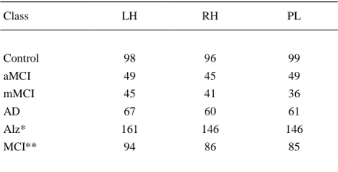
(4) relative areas and chemical shifts across the two sets of spectra. The fitting of the spectral peaks was thus achieved with a priori knowledge of their actual characteristics. The main brain metabolites, choline (Cho), creatine (Cre), N-acetylaspartate (NAA), and myo-inositol (mI) were recorded with this software to get their concentrations. The height and area values for each of these peaks were also obtained in the spectrum with MATLAB software ( The MathWorks, Inc., 2014) in order to evaluate their potential as quantification measures. Fig. 1 displays the typical single-voxel spectroscopy prescription in the right hippocampus from one subject, registered onto a high-resolution T1-weighted image in the sagittal (a), transverse (b) and coronal (c) planes. The resulting spectrum from LCModel software is shown in (d). The spectrum exhibits four distinctive peaks, these being (from right to left) NAA, Cr, Cho and mI.. Fig. 1. Single voxel prescription in the right hippocampus from one subject, registered onto a high-resolution T1 SPGR: sagittal (a), transverse (b) and coronal (c) view. Resulting LCModel spectrum (d).. The high-resolution 3D structural images were segmented into grey matter (GM), white matter (WM) and cerebrospinal fluid (CSF) using SPM8 software (SPM, 2014). After this segmentation, the composition of GM, WM and CSF for each spectroscopic voxel was calculated by localising the 1H-MRS voxel onto the three segmented volumes. 2.3. Dataset and analysis description The dataset was divided into the previously described groups (classes): Control, aMCI, mMCI and AD. Additional classes were created by combining the original ones: Alz (aMCI, mMCI, AD) and MCI (aMCI and mMCI). Moreover, cases from the three different brain locations were analysed: right hippocampus (RH), left hippocampus (LH) and parietal lobe (PL). Table 1 describes the number of cases for each class by brain region. The number of cases varies by regions because some subjects could not complete the spectroscopy protocol.. Table 1. Number of cases for each class and brain region. Class. LH. RH. PL. Control. 98. 96. 99. aMCI. 49. 45. 49. mMCI. 45. 41. 36. AD. 67. 60. 61. Alz*. 161. 146. 146. MCI**. 94. 86. 85. * Alz = aMCI, mMCI, AD. ** MCI = aMCI, mMCI..
(5) A total of 20 attributes resulted from the post-processing analysis: mI_Conc, Cho_Conc, Cre_Conc and NAA_Conc (LCModel concentrations of the 4 metabolites), mI/Cr, Cho/Cr, NAA/Cr and mI/NAA (LCModel ratios), mI_Ampl, Cho_Ampl, Cre_Ampl and NAA_Ampl (Peak amplitudes or heights), mI_Area, Cho_Area, Cre_Area and NAA_Area (Peak areas), Tvol (total volume of the spectroscopic voxel), GMvol, WMvol and CSFvol (GM, WM and CSF volumes of the spectroscopic voxel, respectively). Additional 2 attributes were created as ratios of the volumes: CSFvol/Tvol (CSF volume relative to the total volume of the voxel) and GMvol/Tvol (GM volume related to the total volume of the voxel). Therefore, each case had finally 22 attributes. For each of the 3 brain regions (LH, RH, PL), 5 classes (aMCI, mMCI, AD, Alz, MCI) were used vs. Control in order to test 5 types of classification that could predict any Alzheimer stage cases vs. healthy cases.. 3. Classification methods In order to minimise the influence of bias on the original data during training process, to avoid overfitting and to obtain the generalisation error of the model, the different Weka algorithms were applied using the well-known 10-fold cross-validation technique to split the data. Cross-validation is a statistical method for evaluating and comparing classifiers. The idea behind it is to use a part of the dataset to train the classifier, and thereafter use the remaining samples, as a new and unseen set, to test the performance of the classifier. In the 10-fold cross-validation, samples are divided into 10 folds and subsequently 10 iterations of training and validation are performed, so that each fold is used once and only once for validation. Thus, for each round of cross-validation, the performance of the model can be calculated separately, which decreases the variance of the evaluation. The performance of prediction models for a two-class problem is typically evaluated using a confusion matrix. There are several numbers of well-known accuracy measures for a two-class classifier in the literature. In this work, several scores extracted from the confusion matrix are presented: TP/FP rates (where TP is the number of true positives and FP is the number of false positives), Precision and AUROC values, for both training and validation processes. In the studies performed by Ferri et al., 2009 and Huang and Ling, 2005 it was suggested that, in general, AUROC was the best measure for model comparison. Several experiments were performed in order to select the best models and the classification implementations used in those tests were the ones included in Weka. 3.1. Artificial Neural Networks Artificial Neural Networks (Baxt, 1995, Bishop, 1995, Haykin, 1998 and Krogh, 2008) are flexible, non-linear and multidimensional mathematical systems, easily implemented and handled, capable of solving complex functions in very diverse fields. This technique is based on the simulation of the human cognition process (McCulloch & Pitts, 1943). ANNs have been widely used for different problems, such as data analysis, non-invasive diagnosis in the medical field (Ding et al., 2014 and Resino et al., 2011), linking chemical knowledge (Gomez-Carracedo et al., 2007 and Gómez-Carracedo et al., 2007) to protein function prediction (Fernandez-Lozano et al., 2013, Fernandez-Lozano et al., 2014 and FernandezLozano et al., 2014) or, as mentioned before, for AD classification with morphometric measures (Aguilar et al., 2013 and Escudero et al., 2011). ANNs consist of many simple, interconnected computational units. The knowledge lies in the connections links (weights) between these simple units (neurons). ANNs learn by example and have to be trained to adjust the weights which address the pattern recognition problem. After the training process, ANNs can assign labels to unknown data (not used in the learning process). The simplest kind of feed-forward ANN, where the inputs are directly connected to the outputs with a weight value, is known as single-layer perceptron or perceptron. If the problem is linearly separable, the single-layer perceptron learning algorithm will terminate. A multilayer perceptron (MLP) is a feed-forward neural network for non-linearly separable problems with three layers of neurons (input, hidden and output layer) fully connected to the next one with a nonlinear activation function. The MLP training process is performed by means of a back propagation technique in a supervised learning scheme. The election of a good topology is essential; therefore, most of the problems related to the development of the use of ANN are focused on it. There is no rule to choose the best topology to solve a particular problem, thus different topologies should be tested in order to obtain a final one. This search of topology could be done manually or automatically with other techniques, such as genetic algorithms (Holland, 1975 and Picado et al., 2009) or particle swarm optimisation (Fernandez-Lozano, Seoane, Gestal, Gaunt, & Campbell, 2013)..
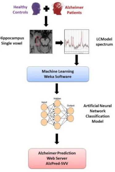
(6) 3.2. Feature selection Feature selection (FS) is a helpful stage prior to classification, for dimensionality reduction, as well as selecting proper features and omitting improper features. The aim of feature selection is to select a subset of extracted variables in order to reduce the number of input variables for the classifier, since the number and relevance of the input variables can affect the performance of the model. An FS approach was performed to find the subset of features best describing the structure of the data. The FS process can answer the main question of how many and which are the most important features to discriminate between Alzheimer dementia and healthy control subjects. In this kind of problems, it is common to perform an FS approach in order to improve the performance of the classification and to choose the best features, solving the classification problem. There are mainly three approaches for FS (Saeys, Inza, & Larrañaga, 2007): Filter, Wrapper and Embedded. For the current study, a Filter approach was used to assess the relevance of features by looking only at the intrinsic properties of the data as a fast and simple computationally approach, independent of the particular classification algorithm. Fig. 2 presents the flow chart of the methodology used in this study: the 22 attributes described above were retrieved for each subject from the full dataset (healthy controls, MCI and AD) using the three 1H-MRS studies. Finally, the best classification model was implemented as a free Web tool entitled “Alzheimer Prediction by Spectroscopy Voxel Volume” (AlzPred-SVV) at http://bioaims.udc.es/AlzPredSVV.php. The tool is based on an HTML/PHP user interface with a Python/Java implementation of the model.. Fig. 2. Flow chart for the calculation of Alzheimer’s disease patient classification using 1H-MRS data and Weka machine-learning techniques and the implementation of the best model as a free Web tool for the prediction of Alzheimer’s..
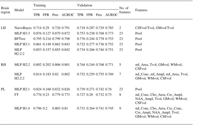
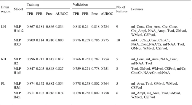
(7) 4. Results In the first step, the information of the 4 classes was used to look for classification results between Alz class (aMCI, mMCI and AD) and Control class, including the 3 pathological classes into a single group (Alz). Table 2 shows these results for each brain region with the following scores for the best models: TP/FP rates, Precision and AUROC values for both training and validation datasets, and the last two columns with the number and name of the features. Note that the best results were achieved in the left hippocampus (LH), followed by the right hippocampus (RH) and the parietal lobe (PL). The best model in the left hippocampus was a Naïve Bayes using estimator classes (John & Langley, 1995) with an AUROC value of 0.783. In the right hippocampus and parietal lobe, the best model was a multilayer perceptron (MLP) with AUROC values of 0.771 and 0.760.. Table 2. Alz (mMCI, aMCI, AD) vs. control classification. Training. Validation. Brain region. Model. LH. NaiveBayes 0.714 0.29 0.726 0.791 MLP H3:3 0.876 0.127 0.879 0.872 BFTree. RH. PL. No. of features. Features. 0.718 0.287 0.729 0.783. 2. CSFvol/Tvol, GMvol/Tvol. 0.753 0.238 0.768 0.773. 23. Pool. 0.795 0.216 0.799 0.798. 0.776 0.244 0.778 0.753. 23. Pool. MLP H3:1 0.861 0.148 0.862 0.843. 0.722 0.277 0.736 0.752. 23. Pool. MLP H2:2:2. 0.853 0.157 0.855 0.842. 0.734 0.266 0.746 0.751. 23. Pool. MLP H2:2 0.802 0.202 0.806 0.801. 0.764 0.244 0.768 0.771. 5. mI_Area, Tvol, GMvol, WMvol, CSFvol. MLP H2:2:2. 0.752 0.259 0.755 0.769. 7. mI_Conc, mI_Ampl, mI_Area, Tvol, GMvol, WMvol, CSFvol. MLP H2:1 0.824 0.168 0.832 0.826. 0.739 0.271 0.742 0.76. 23. Pool. FT. 0.727 0.28 0.732 0.75. 8. mI_Conc, Cho_Area, Cre_Ampl, NAA_Ampl, Tvol, GMvol, WMvol, CSFvol. 0.731 0.264 0.741 0.745. 9. mI_Conc, Cho_Area, Cre_Conc, Cre_Ampl, NAA_Ampl, Tvol, GMvol, WMvol, CSFvol. TPR FPR Prec AUROC TPR FPR Prec AUROC. 0.814 0.183 0.82 0.802. 0.776 0.23 0.779 0.773. MLP H1:4 0.796 0.2. 0.803 0.81. Table 3 presents the results obtained from mMCI vs. Control classification for each brain region. Again, the best AUROC values are obtained in the left hippocampus, but in this case using more features than in the right hippocampus and parietal lobe. Models with AUROC values lower than 0.74 are not presented in this work. This is the reason why there is no table for aMCI vs. Control classification (no significant results have been found). In this particular classification problem, for each brain region the best model found was an MLP with a different number of hidden layers, features and AUROC values of 0.784, 0.754 and 0.764..
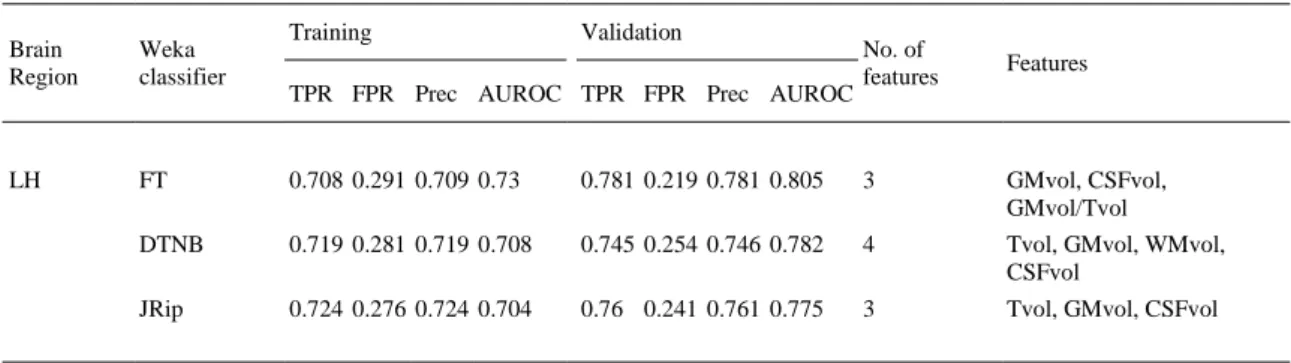
(8) Table 3. mMCI vs. control classification. Brain Model region. LH. RH. PL. Training TPR FPR. Validation Prec AUROC. TPR FPR Prec AUROC. No. of features. Features. MLP 0.867 0.181 0.866 0.834 H1:1:2. 0.818 0.24 0.818 0.784. 9. ml_Conc, Cho_Area, Cre_Conc, Cre_Ampl, NAA_Ampl, Tvol, GMvol, WMvol, CSFvol,. MLP H3:3. 0.909 0.114 0.910 0.880. 0.776 0.259 0.786 0.775. 10. mI/Cr, Cho_Conc, Cho/Cr, NAA_Conc,NAA/Cr, mI/NAA, Tvol, GMvol, WMvol, CSFvol,. MLP H2. 0.796 0.213 0.815 0.817. 0.766 0.267 0.782 0.754. 5. mI_Conc, ml_Area, NAA_Conc, ml/NAA, Tvol. MLP H1:5. 0.847 0.205 0.848 0.827. 0.759 0.271 0.778 0.751. 8. Tvol, GMvol, WMvol, CSFvol, ml/Cr, Cho/Cr, NAA/Cr, ml/NAA. MLP H5:1. 0.874 0.152 0.882 0.854. 0.778 0.258 0.802 0.764. 5. mI_Area, Tvol, GMvol, WMvol, CSFvol. MLP H4:1. 0.911 0.103 0.916 0.874. 0.778 0.258 0.802 0.758. 6. mI_Ampl, mI_Area, Tvol, GMvol, WMvol, CSFvol. The next step consists of finding the most relevant features to discriminate patients affected by Alzheimer’s Disease. A feature selection had been performed for AD vs. Control classification (Table 4) and for MCI (aMCI, mMCI) vs. Control classification (Table 5). The models calculated for AD vs. Control classification presented good results, mainly in the left hippocampus with AUROC values higher than 0.89 (see Table 4). In the left and right hippocampus forest-based models achieved the best results. The best model in the parietal lobe was also an MLP with an AUROC value of 0.839. The aMCI and mMCI groups (Table 5) were joined together because, due to the heterogeneity of MCI, better results might be obtained by grouping all MCI diagnoses into one group. No significant results for the right hippocampus and parietal lobe were found, and the best model in the left hippocampus was a functional tree (Gama, 2004 and Landwehr et al., 2005) with a value of 0.805..
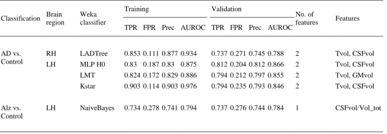
(9) Table 4. Feature selection for AD vs. control classification. Training. Validation. Brain region. Weka classifier. LH. RotationForest 0.964 0.03 0.965 0.996. 0.861 0.143 0.862 0.905. 10. ml/Cr, Cho_Conc, Cho/Cr, NAA_Conc, NAA/Cr, ml/NAA, Tvol, GMvol, WMvol, CSFvol. LogitBoost. 0.903 0.095 0.905 0.951. 0.818 0.181 0.822 0.894. 7. ml_Conc, ml_Altura, ml_Area, Tvol, GMvol, WMvol, CSFvol. MLP H2:2. 0.867 0.129 0.870 0.902. 0.836 0.150 0.846 0.890. 3. Tvol, GMvol, WMvol. RandomForest 0.994 0.004 0.994 1. 0.795 0.203 0.803 0.859. 8. mI_Conc, ml_Altura, ml_Area, Cho_Area, Tvol, GMvol, WMvol, CSFvol. NaiveBayes. 0.821 0.218 0.819 0.874. 0.808 0.226 0.806 0.839. 8. ml/Cr, Cho/Cr, NAA/Cr, ml/NAA, Tvol, GMvol, WMvol, CSFvol. MLP H5:1. 0.949 0.051 0.949 0.935. 0.788 0.195 0.805 0.825. 8. ml/Cr, Cho/Cr, NAA/Cr, ml/NAA, Tvol, GMvol, WMvol, CSFvol. MLP H0. 0.819 0.187 0.823 0.876. 0.781 0.242 0.782 0.839. 8. ml_Conc, Cho_Area, Cre_Ampl, NAA_Ampl, Tvol, GMvol, WMvol, CSFvol. FT. 0.831 0.154 0.843 0.838. 0.794 0.203 0.803 0.831. 8. ml_Conc, Cho_Area, Cre_Ampl, NAA_Ampl, Tvol, GMvol, WMvol, CSFvol. MLP H3:3. 0.869 0.112 0.88 0.885. 0.769 0.249 0.771 0.818. 9. ml_Conc, Cho_Area, Cre_Conc, Cre_Ampl, NAA_Ampl, Tvol, GMvol, WMvol, CSFvol. RH. PL. TPR FPR Prec AUROC TPR FPR Prec AUROC. No. of features. Features. Table 5. Feature selection for MCI (aMCI, mMCI) vs. control classification. Training. Validation. Brain Region. Weka classifier. LH. FT. 0.708 0.291 0.709 0.73. 0.781 0.219 0.781 0.805. 3. GMvol, CSFvol, GMvol/Tvol. DTNB. 0.719 0.281 0.719 0.708. 0.745 0.254 0.746 0.782. 4. Tvol, GMvol, WMvol, CSFvol. JRip. 0.724 0.276 0.724 0.704. 0.76 0.241 0.761 0.775. 3. Tvol, GMvol, CSFvol. TPR FPR Prec AUROC TPR FPR Prec AUROC. No. of features. Features. Finally, Table 6 summarises the best Alzheimer classification models for each brain region based on a maximum of only two features. Therefore, the best Alzheimer model in this study was obtained for the AD vs. Control classification, with the MLP H0 classifier, a linear classifier with no hidden layers that represents a single-layer perceptron (AUROC = 0.866), based on only two variables related to the spectroscopic voxel volumes: Tvol and CSFvol, in the left hippocampus..
(10) Table 6. The best models based on two features.. Classification. AD vs. Control. Alz vs. Control. Training. Brain region. Weka classifier. RH. LADTree. 0.853 0.111 0.877 0.934. LH. MLP H0. 0.83 0.187 0.83 0.875. LMT Kstar NaiveBayes. LH. Validation. No. of features. Features. 0.737 0.271 0.745 0.788. 2. Tvol, CSFvol. 0.812 0.204 0.812 0.866. 2. Tvol, CSFvol. 0.824 0.172 0.829 0.886. 0.794 0.212 0.797 0.855. 2. Tvol, GMvol. 0.903 0.114 0.903 0.976. 0.794 0.235 0.793 0.846. 2. Tvol, CSFvol. 0.734 0.278 0.741 0.794. 0.737 0.276 0.744 0.784. 1. CSFvol/Vol_tot. TPR FPR Prec AUROC TPR FPR Prec AUROC. 5. Discussion The current work presents for the first time the use of machine-learning methods on 1H-MRS data for AD classification. A gender-matched cohort of 260 subjects aged between 57 and 99 years was used to obtain the attribute values for our datasets. The best proposed model to directly predict the AD diagnostic is based on only two variables related to the spectroscopic voxel volumes such as Tvol and CSFvol in the left hippocampus, and a well-known single-layer perceptron. These results are in accordance with previously published works in different fields, indicating that ANN approaches provide higher prediction accuracy for solving classification problems (Mazurowski et al., 2008). All the models were tested using a cross-validation approach. This work demonstrates a robust predictor of AD with an AUROC value of 0.866 and only two features, according to the TPR and FPR values (0.812 and 0.204) achieved in validation and the optimal precision value. This result supports the hypothesis that a single-layer perceptron can predict AD if applied to an unknown dataset. The results also confirm that a single-layer perceptron is an accurate method for the detection of AD. In general, ANNs are potentially a more successful technique than other previously published traditional statistical approaches, when used for predicting the stage of a complex biological process (Almeida, 2002). These good results obtained for the left hippocampus match with the neuropathologic concept of evolution of AD according to the Braak and Braak staging (Braak & Braak, 1991). Atrophy typically starts in the medial temporal and limbic areas, subsequently spreading to parietal association areas and finally to frontal and primary cortices. This interpretation is further supported by accumulating morphometric evidence in MCI and AD patients, proposing hippocampal atrophy as a predictor of subsequent conversion to AD and to discriminate control subjects from AD patients (Ackl et al., 2005 and Dubois et al., 2007). Early changes in hippocampi have been demonstrated with the help of MRI, mainly in the left temporal lobe. As expected, the best results and the AUROC values with higher accuracy are obtained discriminating between AD patients and healthy controls, the two most distant groups. As shown in the results section, MLP seems to achieve good results also for the right hippocampus and parietal lobe. The lack of significant results for the classification of Control and aMCI subjects could be due to the diverse etiology of MCI. Although MCI is a category at high risk of developing dementia, it is becoming progressively evident that under this definition, there is a heterogeneous group of cognitive decline having different outcomes. Some MCI patients never develop dementia and not all AD patients pass through MCI stage. For the same reason, the classification of Control and Alz group has lower accuracy than Control vs. AD. The high heterogeneity of the Alz group with respect to cause and severity of the disease (it includes patients diagnosed with aMCI, mMCI and AD), may reduce the classification success rate and thereby could affect the consistency of the results. The analysis of 1H-MRS data showed that all studied metabolites are relevant for the classification process. By relevance, mI could be mentioned first, since it appears in most of the feature selections, followed by NAA and Cho. These results are in accordance with the literature. As mentioned above, there have been reports of increased mI in subjects with MCI and AD, which is suggestive of an increase in glial content or membrane abnormality in these pathologies. (Parnetti et al., 1997) reported that the increase of mI was correlated with dementia severity and duration. Moreover, several studies reported a.
(11) decrease of NAA values in AD patients and the values achieved for MCI subjects were in between that of healthy subjects and AD patients (Catani et al., 2001 and Kantarci et al., 2000). The results obtained by Tumati et al. (2013) also showed decreases in NAA levels in the posterior cingulate and hippocampus in both the ratio and concentration values. These findings support the role of reduced NAA as a biomarker for the diagnosis of MCI and AD. Although in the results of the current study Cho values seem an important feature to discriminate between groups, the findings in the literature with respect to Cho in MCI and AD subjects were less consistent. The alterations of membrane biochemistry accompanying AD have profound effects on the concentration of various choline-containing compounds. Some studies reported an increase in Cho levels in grey matter (Kantarci et al., 2000 and Pfefferbaum et al., 1999). This increase was associated with decreased memory function (Pfefferbaum et al., 1999) and decreased regional cerebral metabolism (Mielke et al., 2001). However, other studies reported no significant changes in the Cho in subjects with AD (Frederick et al., 1997 and Huang et al., 2001). Note that not only metabolite concentrations had significant results. Ratios with Creatine, mI/Cr, NAA/Cr and Cho/Cr, are shown as selected features in several classifications (see Table 2, Table 3 and Table 4). In some cases, ratios between metabolites are more sensitive in terms of detecting changes (ex. when a metabolite increases and other decreases) and can be more accurate than absolute concentrations. Other than Cr ratios, mI/NAA should be pointed out as another selected feature. Combining the alterations in NAA and mI levels in AD, it was suggested that mI/NAA ratios may provide a basis for a 1H-MRS diagnostic assay (Doraiswamy et al., 1998 and Shonk et al., 1995). The study performed by Wang, Zhao, Yu, Zhou, and Li (2009) revealed significant elevation of mI/NAA ratio in the hippocampus and a significant correlation was found between mI/NAA ratio and cognitive decline. In addition to the concentration and ratios, the metabolite measurements of peak amplitude and area are also relevant to discriminate between groups. The importance of this result is that these measures are not routinely used to quantify spectra, although the area under a metabolite curve in 1H-MRS is directly proportional to the concentration of the metabolite. In the current work, besides the 1H-MRS data, the volumes of GM, WM and CSF have been used within the spectroscopic voxel to consider the problem of variations in tissue composition caused by neurodegeneration. They could affect the variability and the metabolite concentrations. The results obtained for the different tissue volumes of the voxel are very significant (see Table 5 and Table 6). They suggest that just the voxel prescription and the relative proportions of tissue provide a high correlation with the diagnosed groups. Due to the tissue atrophy in MCI and AD pathologies, the brain loses grey and white matter and, as a result, increases the cerebrospinal fluid. This fact is observed by these results showing a strong potential for discriminating between controls, MCI and AD subjects, mainly by the increase of CSF within the voxel with the progression of the disease. The voxel volume variables show more power than metabolites to discriminate between groups, since only two features are required for classifications over 70% (see Table 6). The current results are based on the application for the first time of 1H-MRS data and machinelearning techniques to the classification of AD. Therefore, the results are not easily comparable with previous studies. Besides, the comparison with other studies that have been performed with MRI anatomical data is difficult because they report a range of different accuracies for classification and prediction tasks and they have used different cohorts, features, and techniques. The classification accuracy could be influenced by several factors including both methods and cohort properties: feature extraction methods, feature selection or classification tools, image quality, number of subjects, demographics and clinical diagnosis criteria are also important considerations. Only a few large multicenter cohorts are available in the field of AD. The Alzheimer’s Disease Neuroimaging Initiative (ADNI) is the most commonly used cohort (ADNI, 2015). ADNI is a North American-based study that was launched in 2003 and aimed to recruit 800 adults (approximately 200 cognitively normal older individuals, 400 people with MCI, and 200 people with early AD) to participate in the research and be followed for 2–3 years. ADNI subjects were aged between 55 and 90, and were recruited from over 50 sites across the US and Canada. Many of the recent studies in the field have used this cohort to benefit the comparison between studies. However, ADNI or any other public database has no data from 1H-MRS studies, as using these public datasets for this study or any other study about spectroscopy was not possible. Almost all studies published in the literature about 1H-MRS use their own sample data. Despite all this, the scores obtained with spectroscopic data to classify AD patients and cognitively normal subjects are in agreement with previous studies that use MRI data. The classification accuracy for distinguishing between AD subjects and Control individuals tends to be between 80% and 90%. The accuracies are rarely higher for studies using large sample sizes. Studies achieving close to 100% accuracies are likely to have an over-fitted model, resulting from very small homogenous samples or they may use clinical measures for diagnosing the subjects as input, leading to circularity problems (Falahati et al., 2014)..
(12) The study carried out by Aguilar et al. (2013) compared different multivariate classifiers using MRI data as input for classification of AD vs. Controls out of a total of 345 subjects: 116 AD, 119 MCI and 110 Controls. Similar performance was obtained for the different methods: DT (accuracy = 81.9% and AUROC = 0.78), ANN (accuracy = 84.9% and AUC = 0.88) and SVM (accuracy = 83.6% and AUROC = 0.91). The classification performance was based on 10-fold cross-validation for each classifier, leading to the same input; using the same cohort, different multivariate classifiers tend to perform very similarly. Using SVM, (Abdulkadir et al., 2011) reported an accuracy of 87% for an MRI dataset comprising 417 subjects from the ADNI database, while (Cuingnet et al., 2011) obtained 81% sensitivity and 95% specificity for MRI data from 299 subjects from the same database. The study conducted by Di Deco et al. (2013), with a subset of the cohort used for this study, employed combinations of different MR neuroimaging biomarkers, including 1H-MRS metabolites, to classify AD in its different stages. Regarding the spectroscopic data, they reported accuracies of 74% for discriminating between controls and aMCI, which are similar to the results of the current study, and 77% for discriminating between controls and AD, where the current study presents better accuracies (higher than 85%).. 6. Conclusion The number of features plays an important role in a classification problem. It is necessary to study the relevance in order to suppress noise by means of a feature selection approach. It is known that a model with a high number of features could suffer from over-fitting (Hastie, Tibshirani, & Friedman, 2009) and the current study also looked for a smaller subset with better accuracy results in order to get a better interpretation of the results. Those approaches are applied in order to improve the classification accuracy and to enhance the interpretability of the results. In this work, a single-layer perceptron outperforms the results achieved with other machine-learning techniques included in the Weka algorithms collection and it seems to be more suitable for describing this complex biological system. In conclusion, our study reflects that the best classifier in terms of AUROC is a single-layer perceptron with only two spectroscopic voxel volumes (Tvol and CSFvol) in the left hippocampus, with an AUROC value of 0.866 (with TPR 0.812 and FPR 0.204). The scores obtained are in accordance with previous studies in AD classification (ranging from 80% to 90%). Our results suggest that precise composition of white and grey matter and cerebrospinal fluid is essential in a 1H-MRS study to improve the accuracy of the quantifications and classifications, particularly in those studies involving elder patients and neurodegenerative diseases. However, further investigation involving larger patient cohorts are needed to increase confidence and reproducibility of these methods. As mentioned before, there are different approaches for AD prediction using different types of data. Future research using MRI data, different MR Neuroimaging biomarkers and a combination with some genomic data for clinical tests could be performed following a data fusion scheme (Lanckriet, De Bie, Cristianini, Jordan, & Noble, 2004). One of the main drawbacks of ANN approaches is precisely the impossibility to calculate the real contribution of each feature in the final solution whilst this could be calculated following the aforementioned data fusion approach (Seoane, Day, Gaunt, & Campbell, 2013). The best model was implemented as Alzheimer Prediction by Spectroscopy Voxel Volume (AlzPredSVV) at http://bio-aims.udc.es/AlzPredSVV.php, an easy-to-use web application to validate our model. Such development can be useful for both clinicians and patients. This application is on a free portal that offers theoretical models based on Artificial Intelligence, Computational Biology and Bioinformatics to study complex systems, with the goal of having the largest possible dissemination. The website provides the values of predicted class and error prediction achieved by the model.. Acknowledgements This work is supported by the “Collaborative Project on Medical Informatics (CIMED)” PI13/00280 funded by the Carlos III Health Institute from the Spanish National plan for Scientific and Technical Research and Innovation 2013–2016 and the European Regional Development Fund (FEDER). The authors thank the DEMCAM project team, a multicentre study with patients from different centres for dementia in the Autonomous Region of Madrid..
(13) References Abdulkadir et al., 2011. A. Abdulkadir, B. Mortamet, P. Vemuri, C.R. Jack Jr., G. Krueger, S. Klöppel. Effects of hardware heterogeneity on the performance of SVM Alzheimer’s disease classifier. Neuroimage, 58 (3) (2011), pp. 785–792. Ackl et al., 2005. N. Ackl, M. Ising, Y.A. Schreiber, M. Atiya, A. Sonntag, D.P. Auer, et al. Hippocampal metabolic abnormalities in mild cognitive impairment and Alzheimer’s disease. Neuroscience Letters, 384 (1-2) (2005), pp. 23–28. Adaszewski et al., 2013. S. Adaszewski, J. Dukart, F. Kherif, R. Frackowiak, B. Draganski. How early can we predict Alzheimer’s disease using computational anatomy?. Neurobiology of Aging, 34 (12) (2013), pp. 2815–2826. ADNI, 2015. ADNI, The Alzheimer’s Disease Neuroimaging Initiative (2015). Retrieved 20/02, 2015, from <http://adni.loni.usc.edu/>. Aguilar et al., 2013. C. Aguilar, E. Westman, J. Muehlboeck, P. Mecocci, B. Vellas, M. Tsolaki, et al. Different multivariate techniques for automated classification of MRI data in Alzheimer’s disease and mild cognitive impairment. Psychiatry Research: Neuroimaging, 212 (2) (2013), pp. 89–98. Almeida, 2002. J.S. Almeida. Predictive non-linear modeling of complex data by artificial neural networks. Current Opinion in Biotechnology, 13 (1) (2002), p. 72. Andrade de Oliveira et al., 2015. A. Andrade de Oliveira, M.T. Carthery-Goulart, P.P. Oliveira Junior, D.C. Carrettiero, J.R. Sato. Defining multivariate normative rules for healthy aging using neuroimaging and machine learning: An application to Alzheimer’s disease. Journal of Alzheimer’s Disease, 43 (1) (2015), pp. 201–212. Baxt, 1995. W.G. Baxt. Application of artificial neural networks to clinical medicine. Lancet, 346 (8983) (1995), pp. 1135–1138. Bishop, 1995. C.M. Bishop. Neural networks for pattern recognition. Oxford University Press Inc, New York, NY, USA (1995). Braak and Braak, 1991. H. Braak, E. Braak. Neuropathological stageing of Alzheimer-related changes. Acta Neuropathologica, 82 (4) (1991), pp. 239–259. Catani et al., 2001. M. Catani, A. Cherubini, R. Howard, R. Tarducci, G.P. Pelliccioli, M. Piccirilli, et al.. (1)H-MR spectroscopy differentiates mild cognitive impairment from normal brain aging. Neuroreport, 12 (11) (2001), pp. 2315–2317. Chantal et al., 2004. S. Chantal, C.M. Braun, R.W. Bouchard, M. Labelle, Y. Boulanger. Similar 1H magnetic resonance spectroscopic metabolic pattern in the medial temporal lobes of patients with mild cognitive impairment and Alzheimer disease. Brain Research, 1003 (1–2) (2004), pp. 26–35. Chantal et al., 2002. S. Chantal, M. Labelle, R.W. Bouchard, C.M. Braun, Y. Boulanger. Correlation of regional proton magnetic resonance spectroscopic metabolic changes with cognitive deficits in mild Alzheimer disease. Archives of Neurology, 59 (6) (2002), pp. 955–962. Cho et al., 2012. Y. Cho, J.K. Seong, Y. Jeong, S.Y. Shin, Alzheimer’s Disease Neuroimaging Initiative. Individual subject classification for Alzheimer’s disease based on incremental learning using a spatial frequency representation of cortical thickness data. Neuroimage, 59 (3) (2012), pp. 2217–2230. Coupe et al., 2012. P. Coupe, S.F. Eskildsen, J.V. Manjon, V.S. Fonov, D.L. Collins, Alzheimer’s disease Neuroimaging Initiative. Simultaneous segmentation and grading of anatomical structures for patient’s classification: Application to Alzheimer’s disease. Neuroimage, 59 (4) (2012), pp. 3736–3747. Cuingnet et al., 2011. R. Cuingnet, E. Gerardin, J. Tessieras, G. Auzias, S. Lehéricy, M. Habert, et al. Automatic classification of patients with Alzheimer’s disease from structural MRI: A comparison of ten methods using the ADNI database. Neuroimage, 56 (2) (2011), pp. 766–781. Davies et al., 2008. N.P. Davies, M. Wilson, L.M. Harris, K. Natarajan, S. Lateef, L. MacPherson, et al. Identification and characterisation of childhood cerebellar tumours by in vivo proton MRS. NMR in Biomedicine, 21 (8) (2008), pp. 908–918. de Leon et al., 1993. M.J. de Leon, J. Golomb, A.E. George, A. Convit, C.Y. Tarshish, T. McRae, et al. The radiologic prediction of Alzheimer disease: The atrophic hippocampal formation. AJNR American Journal of Neuroradiology, 14 (4) (1993), pp. 897–906. Devanand et al., 2007. D.P. Devanand, G. Pradhaban, X. Liu, A. Khandji, S. De Santi, S. Segal, et al. Hippocampal and entorhinal atrophy in mild cognitive impairment: Prediction of Alzheimer disease. Neurology, 68 (11) (2007), pp. 828–836. Di Deco et al., 2013. J. Di Deco, A.M. González, J. Díaz, V. Mato, D. García-Frank, J. Álvarez-Linera, et al. Machine learning and social network analysis applied to Alzheimer’s disease biomarkers. Current Topics in Medicinal Chemistry, 13 (5) (2013), pp. 652–662. Ding et al., 2014. H. Ding, Q. Lu, H. Gao, Z. Peng. Non-invasive prediction of hemoglobin levels by principal component and back propagation artificial neural network. Biomedical Optics Express, 5 (4) (2014), pp. 1145– 1152. Doraiswamy et al., 1998. P.M. Doraiswamy, H.C. Charles, K.R. Krishnan. Prediction of cognitive decline in early Alzheimer’s disease. Lancet, 352 (9141) (1998), p. 1678. Dubois et al., 2007. B. Dubois, H.H. Feldman, C. Jacova, S.T. Dekosky, P. Barberger-Gateau, J. Cummings, et al. Research criteria for the diagnosis of Alzheimer’s disease: Revising the NINCDS-ADRDA criteria. Lancet Neurology, 6 (8) (2007), pp. 734–746. Dyrba et al., 2013. M. Dyrba, M. Ewers, M. Wegrzyn, I. Kilimann, C. Plant, A. Oswald, et al. Robust automated detection of microstructural white matter degeneration in Alzheimer’s disease using machine learning classification of multicenter DTI data. PloS One, 8 (5) (2013), p. e64925..
(14) Ernst and Kellis, 2015. Ernst, J., & Kellis, M. (2015). Large-scale imputation of epigenomic datasets for systematic annotation of diverse human tissues. Nat Biotech, advance online publication. Ernst et al., 1997. T. Ernst, L. Chang, R. Melchor, C.M. Mehringer. Frontotemporal dementia and early Alzheimer disease: Differentiation with frontal lobe H-1 MR spectroscopy. Radiology, 203 (3) (1997), pp. 829–836. Escudero et al., 2011. Escudero, J., Zajicek, J. P., Ifeachor, E., & Alzheimer’s Disease Neuroimaging Initiative. (2011). Machine learning classification of MRI features of Alzheimer’s disease and mild cognitive impairment subjects to reduce the sample size in clinical trials. In Conference proceedings: Annual international conference of the IEEE engineering in medicine and biology society. IEEE engineering in medicine and biology society. Annual conference (pp. 7957–7960). Eskildsen et al., 2013. S.F. Eskildsen, P. Coupe, D. Garcia-Lorenzo, V. Fonov, J.C. Pruessner, D.L. Collins, et al. Prediction of Alzheimer’s disease in subjects with mild cognitive impairment from the ADNI cohort using patterns of cortical thinning. Neuroimage, 65 (2013), pp. 511–521. Falahati et al., 2014. F. Falahati, E. Westman, A. Simmons. Multivariate data analysis and machine learning in Alzheimer’s disease with a focus on structural magnetic resonance imaging. Journal of Alzheimer’s Disease: JAD, 41 (3) (2014), pp. 685–708. Falini et al., 2005. A. Falini, M. Bozzali, G. Magnani, G. Pero, A. Gambini, B. Benedetti, et al. A whole brain MR spectroscopy study from patients with Alzheimer’s disease and mild cognitive impairment. NeuroImage, 26 (4) (2005), pp. 1159–1163. Farhan et al., 2014. S. Farhan, M.A. Fahiem, H. Tauseef. An ensemble-of-classifiers based approach for early diagnosis of Alzheimer’s disease: Classification using structural features of brain images. Computational and Mathematical Methods in Medicine, 2014 (2014), p. 862307. Fernandez-Lozano et al., 2014. C. Fernandez-Lozano, E. Fernandez-Blanco, K. Dave, N. Pedreira, M. Gestal, J. Dorado, et al. Improving enzyme regulatory protein classification by means of SVM-RFE feature selection. Molecular Biosystems, 10 (5) (2014), pp. 1063–1071. Fernandez-Lozano et al., 2014. C. Fernandez-Lozano, M. Gestal, H. Gonzalez-Diaz, J. Dorado, A. Pazos, C.R. Munteanu. Markov mean properties for cell death-related protein classification. Journal of Theoretical Biology, 349 (2014), pp. 12–21. Fernandez-Lozano et al., 2013. C. Fernandez-Lozano, M. Gestal, N. Pedreira-Souto, L. Postelnicu, J. Dorado, C.R. Munteanu. Kernel-based feature selection techniques for transport proteins based on star graph topological indices. Current Topics in Medicinal Chemistry, 13 (14) (2013), pp. 1681–1691. Fernandez-Lozano et al., 2013. C. Fernandez-Lozano, J. Seoane, M. Gestal, T. Gaunt, C. Campbell. Texture classification using kernel-based techniques. Lecture Notes in Computer Science, 7902 (2013), pp. 427–434. Ferri et al., 2009. C. Ferri, J. Hernández-Orallo, R. Modroiu. An experimental comparison of performance measures for classification. Pattern Recognition Letters, 30 (1) (2009), pp. 27–38. Folstein et al., 1975. M.F. Folstein, S.E. Folstein, P.R. McHugh. “Mini-mental state”. A practical method for grading the cognitive state of patients for the clinician. Journal of Psychiatric Research, 12 (3) (1975), pp. 189–198. Frederick et al., 2004. B.D. Frederick, I.K. Lyoo, A. Satlin, K.H. Ahn, M.J. Kim, D.A. Yurgelun-Todd, et al. In vivo proton magnetic resonance spectroscopy of the temporal lobe in Alzheimer’s disease. Progress in Neuropsychopharmacology & Biological Psychiatry, 28 (8) (2004), pp. 1313–1322. Frederick et al., 1997. B.B. Frederick, A. Satlin, D.A. Yurgelun-Todd, P.F. Renshaw. In vivo proton magnetic resonance spectroscopy of Alzheimer’s disease in the parietal and temporal lobes. Biological Psychiatry, 42 (2) (1997), pp. 147–150. Gama, 2004. J. Gama. Functional trees. Machine Learning, 55 (3) (2004), pp. 219–250. Gómez-Carracedo et al., 2007. M.P. Gómez-Carracedo, M. Gestal, J. Dorado, J.M. Andrade. Linking chemical knowledge and genetic algorithms using two populations and focused multimodal search. Chemometrics and Intelligent Laboratory Systems, 87 (2007), pp. 173–184. Gomez-Carracedo et al., 2007. M.P. Gomez-Carracedo, M. Gestal, J. Dorado, J.M. Andrade. Chemically driven variable selection by focused multimodal genetic algorithms in mid-IR spectra. Analytical and Bioanalytical Chemistry, 389 (7–8) (2007), pp. 2331–2342. Grundman et al., 2004. M. Grundman, R.C. Petersen, S.H. Ferris, R.G. Thomas, P.S. Aisen, D.A. Bennett, et al. Mild cognitive impairment can be distinguished from Alzheimer disease and normal aging for clinical trials. Archives of Neurology, 61 (1) (2004), pp. 59–66. Hall et al., 2009. M. Hall, E. Frank, G. Holmes, B. Pfahringer, P. Reutemann, I.H. Witten. The WEKA data mining software: An update. ACM SIGKDD Explorations Newsletter, 11 (1) (2009), pp. 10–18. Haller et al., 2010. S. Haller, D. Nguyen, C. Rodriguez, J. Emch, G. Gold, A. Bartsch, et al. Individual prediction of cognitive decline in mild cognitive impairment using support vector machine-based analysis of diffusion tensor imaging data. Journal of Alzheimer’s Disease, 22 (1) (2010), pp. 315–327. Hamou et al., 2011. A. Hamou, A. Simmons, M. Bauer, B. Lewden, Y. Zhang, L. Wahlund, et al. Cluster analysis of MR imaging in Alzheimer’s disease using decision tree refinement. International Journal of Artificial Intelligence, 6 (s11) (2011), pp. 90–99. Hampel et al., 2008. H. Hampel, K. Bürger, S.J. Teipel, A.L.W. Bokde, H. Zetterberg, K. Blennow. Core candidate neurochemical and imaging biomarkers of Alzheimer’s disease. Alzheimer’s and Dementia, 4 (1) (2008), pp. 38– 48. Hastie et al., 2009. T. Hastie, R. Tibshirani, J. Friedman. The elements of statistical learning: Data mining, inference, and prediction. (2nd ed.)Springer, New York (2009). Haykin, 1998. S. Haykin. Neural networks: A comprehensive foundation. (2nd ed.)Prentice Hall PTR, Upper Saddle River, NJ, USA (1998)..
(15) Holland, 1975. J.H. Holland. Adaptation in natural and artificial systems: An introductory analysis with applications to biology, control, and artificial intelligence. University of Michigan Press (1975). Holland et al., 2009. D. Holland, J.B. Brewer, D.J. Hagler, C. Fennema-Notestine, A.M. Dale. Subregional neuroanatomical change as a biomarker for Alzheimer’s disease. Proceedings of the National Academy of Sciences of the United States of America, 106 (49) (2009), pp. 20954–20959. Huang et al., 2001. W. Huang, G.E. Alexander, L. Chang, H.U. Shetty, J.S. Krasuski, S.I. Rapoport, et al. Brain metabolite concentration and dementia severity in Alzheimer’s disease: A (1)H MRS study. Neurology, 57 (4) (2001), pp. 626–632. Huang and Ling, 2005. J. Huang, C.X. Ling. Using AUC and accuracy in evaluating learning algorithms. IEEE Transactions on Knowledge and Data Engineering, 17 (3) (2005), pp. 299–310. Hughes et al., 1982. C.P. Hughes, L. Berg, W.L. Danziger, L.A. Coben, R.L. Martin. A new clinical scale for the staging of dementia. The British Journal of Psychiatry: The Journal of Mental Science, 140 (1982), pp. 566–572. John and Langley, 1995. John, G., & Langley, P. (1995). Estimating continuous distributions in bayesian classifiers. In Proceedings of the eleventh conference on uncertainty in artificial intelligence (pp. 338–345). Kantarci et al., 2000. K. Kantarci, C.R. Jack Jr, Y.C. Xu, N.G. Campeau, P.C. O’Brien, G.E. Smith, et al. Regional metabolic patterns in mild cognitive impairment and Alzheimer’s disease: A 1H MRS study. Neurology, 55 (2) (2000), pp. 210–217. Kantarci et al., 2007. K. Kantarci, S.D. Weigand, R.C. Petersen, B.F. Boeve, D.S. Knopman, J. Gunter, et al. Longitudinal 1H MRS changes in mild cognitive impairment and Alzheimer’s disease. Neurobiology of Aging, 28 (9) (2007), pp. 1330–1339. Kloppel et al., 2008. S. Kloppel, C.M. Stonnington, C. Chu, B. Draganski, R.I. Scahill, J.D. Rohrer, et al. Automatic classification of MR scans in Alzheimer’s disease. Brain: A Journal of Neurology, 131 (Pt 3) (2008), pp. 681– 689. Koikkalainen et al., 2011. J. Koikkalainen, J. Lötjönen, L. Thurfjell, D. Rueckert, G. Waldemar, H. Soininen. Multitemplate tensor-based morphometry: Application to analysis of Alzheimer’s disease. Neuroimage, 56 (3) (2011), pp. 1134–1144. Korf et al., 2004. E.S. Korf, L.O. Wahlund, P.J. Visser, P. Scheltens. Medial temporal lobe atrophy on MRI predicts dementia in patients with mild cognitive impairment. Neurology, 63 (1) (2004), pp. 94–100. Kosmicki et al., 2015. J.A. Kosmicki, V. Sochat, M. Duda, D.P. Wall. Searching for a minimal set of behaviors for autism detection through feature selection-based machine learning. Translational Psychiatry, 5 (2015), p. e514. Krogh, 2008. A. Krogh. What are artificial neural networks?. Nature Biotechnology, 26 (2) (2008), pp. 195–197. Lanckriet et al., 2004. G.R.G. Lanckriet, T. De Bie, N. Cristianini, M.I. Jordan, W.S. Noble. A statistical framework for genomic data fusion. Bioinformatics, 20 (16) (2004), pp. 2626–2635. Landwehr et al., 2005. N. Landwehr, M. Hall, E. Frank. Logistic model trees. Machine Learning, 59 (1–2) (2005), pp. 161–205. Lin et al., 2005. A. Lin, B.D. Ross, K. Harris, W. Wong. Efficacy of proton magnetic resonance spectroscopy in neurological diagnosis and neurotherapeutic decision making. NeuroRx: The Journal of the American Society for Experimental NeuroTherapeutics, 2 (2) (2005), pp. 197–214. Liu et al., 2013. X. Liu, D. Tosun, M.W. Weiner, N. Schuff, Alzheimer’s Disease Neuroimaging Initiative. Locally linear embedding (LLE) for MRI based Alzheimer’s disease classification. Neuroimage, 83 (2013), pp. 148–157. Magnin et al., 2009. B. Magnin, L. Mesrob, S. Kinkingnehun, M. Pelegrini-Issac, O. Colliot, M. Sarazin, et al. Support vector machine-based classification of Alzheimer’s disease from whole-brain anatomical MRI. Neuroradiology, 51 (2) (2009), pp. 73–83. Mazurowski et al., 2008. M.A. Mazurowski, P.A. Habas, J.M. Zurada, J.Y. Lo, J.A. Baker, G.D. Tourassi. Training neural network classifiers for medical decision making: The effects of imbalanced datasets on classification performance. Neural Networks: The Official Journal of the International Neural Network Society, 21 (2–3) (2008), pp. 427–436. McCulloch and Pitts, 1943. W.S. McCulloch, W. Pitts. A logical calculus of the ideas immanent in nervous activity. Bulletin of Mathematical Biology, 5 (4) (1943), pp. 115–133. McEvoy et al., 2011. L.K. McEvoy, D. Holland, D.J. Hagler Jr., C. Fennema-Notestine, J.B. Brewer, A.M. Dale, et al. Mild cognitive impairment: Baseline and longitudinal structural MR imaging measures improve predictive prognosis. Radiology, 259 (3) (2011), pp. 834–843. McKhann et al., 1984. G. McKhann, D. Drachman, M. Folstein, R. Katzman, D. Price, E.M. Stadlan. Clinical diagnosis of Alzheimer’s disease: Report of the NINCDS-ADRDA work group under the auspices of department of health and human services task force on Alzheimer’s disease. Neurology, 34 (7) (1984), pp. 939–944. Metastasio et al., 2006. A. Metastasio, P. Rinaldi, R. Tarducci, E. Mariani, F.T. Feliziani, A. Cherubini, et al. Conversion of MCI to dementia: Role of proton magnetic resonance spectroscopy. Neurobiology of Aging, 27 (7) (2006), pp. 926–932. Mielke et al., 2001. R. Mielke, H.H. Schopphoff, H. Kugel, U. Pietrzyk, W. Heindel, J. Kessler, et al. Relation between 1H MR spectroscopic imaging and regional cerebral glucose metabolism in Alzheimer’s disease. The International Journal of Neuroscience, 107 (3–4) (2001), pp. 233–245. Miller et al., 1993. B.L. Miller, R.A. Moats, T. Shonk, T. Ernst, S. Woolley, B.D. Ross. Alzheimer disease: Depiction of increased cerebral myo-inositol with proton MR spectroscopy. Radiology, 187 (2) (1993), pp. 433–437. Moats et al., 1994. R.A. Moats, T. Ernst, T.K. Shonk, B.D. Ross. Abnormal cerebral metabolite concentrations in patients with probable Alzheimer disease. Magnetic Resonance in Medicine, 32 (1) (1994), pp. 110–115..
(16) Modrego and Fayed, 2012. P.J. Modrego, N. Fayed. Longitudinal magnetic resonance spectroscopy as marker of cognitive deterioration in mild cognitive impairment. American Journal of Alzheimer’s Disease and Other Dementias, 26 (8) (2012), pp. 631–636. O’Dwyer et al., 2012. L. O’Dwyer, F. Lamberton, A.L. Bokde, M. Ewers, Y.O. Faluyi, C. Tanner, et al. Using support vector machines with multiple indices of diffusion for automated classification of mild cognitive impairment. PloS One, 7 (2) (2012), p. e32441. Opstad et al., 2007. K.S. Opstad, C. Ladroue, B.A. Bell, J.R. Griffiths, F.A. Howe. Linear discriminant analysis of brain tumour 1H MR spectra: A comparison of classification using whole spectra versus metabolite quantification. NMR in Biomedicine, 20 (8) (2007), pp. 763–770. Parnetti et al., 1997. L. Parnetti, R. Tarducci, O. Presciutti, D.T. Lowenthal, M. Pippi, B. Palumbo, et al. Proton magnetic resonance spectroscopy can differentiate Alzheimer’s disease from normal aging. Mechanisms of Ageing and Development, 97 (1) (1997), pp. 9–14. Pearson et al., 1985. R.C. Pearson, M.M. Esiri, R.W. Hiorns, G.K. Wilcock, T.P. Powell. Anatomical correlates of the distribution of the pathological changes in the neocortex in Alzheimer disease. Proceedings of the National Academy of Sciences of the United States of America, 82 (13) (1985), pp. 4531–4534. Petersen et al., 1999. R.C. Petersen, G.E. Smith, S.C. Waring, R.J. Ivnik, E.G. Tangalos, E. Kokmen. Mild cognitive impairment: Clinical characterization and outcome. Archives of Neurology, 56 (3) (1999), pp. 303–308. Pfefferbaum et al., 1999. A. Pfefferbaum, E. Adalsteinsson, D. Spielman, E.V. Sullivan, K.O. Lim. In vivo brain concentrations of N-acetyl compounds, creatine, and choline in Alzheimer disease. Archives of General Psychiatry, 56 (2) (1999), pp. 185–192. Picado et al., 2009. Picado, H., Gestal, M., Lau, N., Reis, L., & Tomé, A. M. (2009). Automatic generation of biped walk behavior using genetic algorithms. Bio-inspired systems: Computational and ambient intelligence, Lecture notes in computer science, 5517, pp. 805–812. Plant et al., 2010. C. Plant, S.J. Teipel, A. Oswald, C. Bohm, T. Meindl, J. Mourao-Miranda, et al. Automated detection of brain atrophy patterns based on MRI for the prediction of Alzheimer’s disease. NeuroImage, 50 (1) (2010), pp. 162–174. Provencher, 2001. S.W. Provencher. Automatic quantitation of localized in vivo 1H spectra with LCModel. NMR in Biomedicine, 14 (4) (2001), pp. 260–264. Querbes et al., 2009. O. Querbes, F. Aubry, J. Pariente, J.A. Lotterie, J.F. Demonet, V. Duret, et al. Early diagnosis of Alzheimer’s disease using cortical thickness: Impact of cognitive reserve. Brain: A Journal of Neurology, 132 (Pt 8) (2009), pp. 2036–2047. Raji et al., 2009. C.A. Raji, O.L. Lopez, L.H. Kuller, O.T. Carmichael, J.T. Becker. Age, Alzheimer disease, and brain structure. Neurology, 73 (22) (2009), pp. 1899–1905. Raschke et al., 2013. F. Raschke, N.P. Davies, M. Wilson, A.C. Peet, F.A. Howe. Classification of single-voxel 1H spectra of childhood cerebellar tumors using LCModel and whole tissue representations. Magnetic Resonance in Medicine, 70 (1) (2013), pp. 1–6. Raschke et al., 2012. F. Raschke, E. Fuster-Garcia, K.S. Opstad, F.A. Howe. Classification of single-voxel 1H spectra of brain tumours using LCModel. NMR in Biomedicine, 25 (2) (2012), pp. 322–331. Resino et al., 2011. S. Resino, J.A. Seoane, J.M. Bellon, J. Dorado, F. Martin-Sanchez, E. Alvarez, et al. An artificial neural network improves the non-invasive diagnosis of significant fibrosis in HIV/HCV coinfected patients. The Journal of Infection, 62 (1) (2011), pp. 77–86. Ross and Sachdev, 2004. A.J. Ross, P.S. Sachdev. Magnetic resonance spectroscopy in cognitive research. Brain Research. Brain Research Reviews, 44 (2–3) (2004), pp. 83–102. Saeys et al., 2007. Y. Saeys, I. Inza, P. Larrañaga. A review of feature selection techniques in bioinformatics. Bioinformatics, 23 (19) (2007), pp. 2507–2517. Schuff et al., 2002. N. Schuff, A.A. Capizzano, A.T. Du, D.L. Amend, J. O’Neill, D. Norman, et al. Selective reduction of N-acetylaspartate in medial temporal and parietal lobes in AD. Neurology, 58 (6) (2002), pp. 928– 935. Seoane et al., 2013. J.A. Seoane, I.N.M. Day, T.R. Gaunt, C. Campbell. A pathway-based data integration framework for prediction of disease progression. Bioinformatics (2013) (Oxford, England). Shonk et al., 1995. T.K. Shonk, R.A. Moats, P. Gifford, T. Michaelis, J.C. Mandigo, J. Izumi, et al. Probable Alzheimer disease: Diagnosis with proton MR spectroscopy. Radiology, 195 (1) (1995), pp. 65–72. Siger et al., 2009. M. Siger, N. Schuff, X. Zhu, B.L. Miller, M.W. Weiner. Regional myo-inositol concentration in mild cognitive impairment using 1H magnetic resonance spectroscopic imaging. Alzheimer Disease and Associated Disorders, 23 (1) (2009), pp. 57–62. SPM, 2014. SPM (2014). Statistical Parametric Mapping The Wellcome Trust Centre for Neuroimaging at University College of London. Retrieved 12/05, 2014, from <http://www.fil.ion.ucl.ac.uk/spm/>. Teipel et al., 2007. S.J. Teipel, C. Born, M. Ewers, A.L. Bokde, M.F. Reiser, H.J. Moller, et al. Multivariate deformation-based analysis of brain atrophy to predict Alzheimer’s disease in mild cognitive impairment. NeuroImage, 38 (1) (2007), pp. 13–24. The MathWorks, inc., 2014. The MathWorks, inc. (2014). Retrieved 12/05, 2014, from <http://www.mathworks.com/>. Tong et al., 2014. T. Tong, R. Wolz, Q. Gao, R. Guerrero, J.V. Hajnal, D. Rueckert. Multiple instance learning for classification of dementia in brain MRI. Medical Image Analysis, 18 (5) (2014), pp. 808–818. Tumati et al., 2013. S. Tumati, S. Martens, A. Aleman. Magnetic resonance spectroscopy in mild cognitive impairment: Systematic review and meta-analysis. Neuroscience and Biobehavioral Reviews, 37 (10 Pt 2) (2013), pp. 2571–2586..
(17) Valenzuela and Sachdev, 2001. M.J. Valenzuela, P. Sachdev. Magnetic resonance spectroscopy in AD. Neurology, 56 (5) (2001), pp. 592–598. Varol et al., 2012. Varol, E., Gaonkar, B., Erus, G., Schultz, R., & Davatzikos, C. (2012). Feature ranking based nested support vector machine ensemble for medical image classification. In Proceedings/IEEE international symposium on biomedical imaging: From nano to macro. IEEE international symposium on biomedical imaging (pp. 146–149). Vemuri et al., 2008. P. Vemuri, J.L. Gunter, M.L. Senjem, J.L. Whitwell, K. Kantarci, D.S. Knopman, et al. Alzheimer’s disease diagnosis in individual subjects using structural MR images: Validation studies. NeuroImage, 39 (3) (2008), pp. 1186–1197. Visser et al., 2002. P.J. Visser, F.R. Verhey, P.A. Hofman, P. Scheltens, J. Jolles. Medial temporal lobe atrophy predicts Alzheimer’s disease in patients with minor cognitive impairment. Journal of Neurology, Neurosurgery, and Psychiatry, 72 (4) (2002), pp. 491–497. Waldman and Rai, 2003. A.D. Waldman, G.S. Rai. The relationship between cognitive impairment and in vivo metabolite ratios in patients with clinical Alzheimer’s disease and vascular dementia: A proton magnetic resonance spectroscopy study. Neuroradiology, 45 (8) (2003), pp. 507–512. Wang et al., 2009. Z. Wang, C. Zhao, L. Yu, W. Zhou, K. Li. Regional metabolic changes in the hippocampus and posterior cingulate area detected with 3-tesla magnetic resonance spectroscopy in patients with mild cognitive impairment and Alzheimer disease. Acta Radiologica (Stockholm, Sweden: 1987), 50 (3) (2009), pp. 312–319. Watanabe et al., 2010. T. Watanabe, A. Shiino, I. Akiguchi. Absolute quantification in proton magnetic resonance spectroscopy is useful to differentiate amnesic mild cognitive impairment from Alzheimer’s disease and healthy aging. Dementia and Geriatric Cognitive Disorders, 30 (1) (2010), pp. 71–77. Westman et al., 2011. E. Westman, A. Simmons, Y. Zhang, J.S. Muehlboeck, C. Tunnard, Y. Liu, et al. Multivariate analysis of MRI data for Alzheimer’s disease, mild cognitive impairment and healthy controls. Neuroimage, 54 (2) (2011), pp. 1178–1187. Young et al., 2013. J. Young, M. Modat, M.J. Cardoso, A. Mendelson, D. Cash, S. Ourselin. Accurate multimodal probabilistic prediction of conversion to Alzheimer’s disease in patients with mild cognitive impairment. NeuroImage: Clinical, 2 (0) (2013), pp. 735–745..
(18)
Figure
+3
Documento similar