Innovation, catch up, and leadership in science based industries

♣_{We would like to thank Jose Ignacio Santos for his very valuable help and technical support.}

Innovation, Catch-up and Leadership in Science-Based Industries

Isabel Almudi1_{, Francisco Fatas-Villafranca}1 _{and Luis R. Izquierdo}2 1_{University of Zaragoza} 2_{University of Burgos & InSiSoc}

Abstract

In this paper, we seek to shed new light on the sources of industrial leadership and catch-up in science-based industries. We propose an evolutionary model which incorporates scientists' training and migration, endogenous R&D decisions and the possibility of funding capital accumulation through debt. The analysis of the model allows us to characterize a robust pattern of industrial catch-up. Likewise, the sensitivity analysis shows which parameters act as pro-catch up factors or slow down the process. The identification of stationary-state conditions of the model helps us to interpret the simulations, and highlights crucial interactions between technology-supporting institutions and market demand at the basis of industrial catch-up. Finally, the robustness analysis reveals further interdependencies among innovation, scientist mobility and demand.

Keywords: Innovation, Catch-up; Industrial leadership; Evolutionary Economics.

JEL-Code: O33; B52

1

Introduction

At certain times in the evolution of important science-based industries such as chemicals, semiconductors, pharmaceuticals, medical devices or computer hardware and software, a few firms from one nation (or from a small number of nations) have achieved commercial and technological leadership and then gone on to maintain it for some time (Malerba, 1985; Nelson and Wright, 1992). Frequently, though, these apparently solid leadership positions have been altered by surprising leadership shifts (Amsden, 2001; Murmann, 2003). Previous studies on the sources of industrial leadership have highlighted the role of strategic, technological and institutional factors in these processes (Nelson, 2008). More recently, co-evolution models have been proposed in which the sources of industrial leadership and economic catch-up are formally analyzed (Malerba et al. 2008; Fatas-Villafranca et al. 2008, 2009).

2

Recently, Thorn and Holm-Nielsen (2006) have shown that the high demand for industrial scientists has led to an increase in skilled migration in recent years. In fact, firms taking on highly-skilled foreign-trained scientists have always enjoyed well-known advantages (Mazzoleni and Nelson, 2007). For example, the development of Japan in the 20th _Century was helped by industrial researchers who had been trained abroad. More recently, the role of American-trained talent in the rise of Far-Eastern microelectronics was very significant (Hamilton and Glain, 1995). Nowadays, the circulation of talent among Silicon Valley, Sao Paulo in Brazil, Hsinchu in Taiwan, Singapore, Bangalore in India, Eindhoven or Frankfurt in Europe, and Shangai in China is transforming industrial relationships at a global scale (Zhang, 2003; Khadria, 2004; Saxenian, 2006).

Taking all this into account, we incorporate the international mobility of scientists into an evolutionary model of industrial leadership. Our model presents a process of market competition in a worldwide science-based sector. We assume that price-making (for-profit) firms, each one with a distinct national identity, compete at a global level in price and product performance. They improve their products through R&D-based innovation activities, for which they need to contract scientists specialized in relevant disciplines for the industry. Scientists in the model are trained in national university systems and they can choose between staying in their home nation –joining a national firm– or emigrating to work for a foreign firm. We suppose that, when emigrating, they are attracted by better monetary conditions and/or the possibility of a better development of their work. Certain national peculiarities in the model (such as University policies or the role of institutions supporting the advance of knowledge), as well as firms' R&D spending (which evolves endogenously, driven by certain learning mechanisms), determine the different monetary and non-monetary working conditions for scientists in the different nations.

3

Let us notice that our model is connected to certain challenges in evolutionary economics. Thus, firstly, we formally link several evolutionary processes (firms' market competition and scientists' migrations at a worldwide level) within one co-evolutionary analytical framework (Malerba, 2006). Secondly, we study the interactive role of innovation, university research, and training in industrial dynamics by incorporating a Nelson-Phelps type innovation function (Nelson and Phelps, 1966). Finally, we agree with Silverberg and Verspagen (2005) in that it may be the time to move towards a new generation of evolutionary models. Thus, we propose a model which incorporates fresh theoretical mechanisms, and we analyze it from a standard scenario inspired by the so-called "Asian miracle".

Bearing in mind that we seek to understand the sources of leadership and industrial catch-up in science-based sectors, we run the model from the standard scenario, and we characterize a type of catch-up process presenting the following features:

a. The emergent firms enjoy an initial advantage in prices which they manage to transform into technological convergence during the process.

b. For the technological convergence to take place, it is essential that emergent nations can count on support from science-related institutions offering access to the worldwide technological frontier.

c. If the aforementioned supporting institutions exist, the Nelson-Phelps-type innovation function ensures that the emergent firms enjoy an initial advantage in R&D productivity.

d. If the emergent firms gradually increase their R&D spending, then the advantage in R&D productivity gives way to a convergence in salaries.

e. In addition, a sufficient effort in educational expenditure, together with the advantage in R&D productivity and the convergence in salaries, lead to an increase in the share of scientists working at the emergent industries. Then, technological convergence and catch-up occur.

4

Afterwards, we carry out a sensitivity analysis which allows us to detail which parameters act as pro-catch-up factors and which slow down or even prevent catch-up. We also present a robustness analysis which shows that our results are solid. Additionally, we obtain some mathematical results that guide the design and interpretation of the simulations. These formal results highlight new properties of the model. Specifically, we identify some stationary-state conditions revealing that technology-supporting institutions and market demand interact in a crucial way at the basis of industrial catch-up.

The paper is organized as follows. We present the model in Section 2. In Section 3, we outline an overview of the dynamics and we present some formal results. Section 4, is devoted to the computational analysis. Finally, we summarize our conclusions.

2

The Model

In order to simplify the model's presentation, we will classify our assumptions into five subsections: competitiveness, demand, growth, financing and innovation.

2.1

The Firms' Competitiveness

Let us assume that there are n (i=1,...,n) firms, each one with a different national identity, competing at a worldwide level in a science-based sector. There is one firm per nation, so we can identify the representative firm of nation i with the i-th national industry.

We assume that the firms compete over price1p_i(t)and product performance x_i(t) (quality, reliability, size, speed, precision, etc.). Regarding prices, we will assume that firms set prices applying a margin to the unit cost (larger margins for greater market powers). Denoting the margin as a function of the firm's market share by m(si(t)) and the total cost per output unit by ci(t), we assume that:

0 ,1 ) 0 ( , 1 )) ( ( ,) ( )) ( ( )

(t =m s t c t m s t ≥ m = m′>

pi i i i

For formal convenience, we will consider the following pricing routine which verifies the aforementioned conditions (Fatas-Villafranca and Saura, 2004).

) ( )) ( 1 ( )

(t s t c t

5

From (1), it is straightforward that firm i's unit profit is )

Regarding performance (xi(t)) we will establish, later, how firms improve their products through R&D-based technological innovations. For now, given the vector (pi(t),xi(t)), we can define the level of competitiveness of firm i’s product (as consumers perceive it in the global market) in the following way:

(

)

( )

This formula captures the fact that consumers value both high levels of performance and low prices. The subjective relativity implied by the terms “high” and “low” is quantified using the average across the different products, whilst the trade-off between performance and price is regulated by parameter α (the price-performance sensitivity of demand).

2.2

Demand Transformation

There is demand-driven production and growth in our model. Regarding the demand-side of the market, we consider that the global demand (Qd(t)_{) grows at a constant and} exogenous rate g > 0, starting out from an initial level Q(0). Likewise, as s_i(t) is the proportion of global demand supplied by firm i at moment t –that is, its market share– we can see that the instantaneous demand of firm i will be:

If we consider that the consumers/users interact among themselves, observing each other and disseminating information regarding prices and performances of different products, we can assume that there will be a gradual process of demand transformation. That is, consumers will withdraw their demand from certain firms and pass it on to others with a higher level of competitiveness γi(t). Drawing on Metcalfe (1998), we propose that this process of demand transformation can be represented by2

1 _{We use physical capital as numeraire.}

:

6

Thus, it is clear that those firms with higher than average levels of competitiveness will tend to capture a greater proportion of the demand, thus reaching above-average demand growth rates d

i

g .

2.3

Production and Growth

Let us see how production and growth fit the evolution of demand. Starting out from a supply-demand equilibrium for each firm3 _{(0) (0)} s₍₀₎

firm's growth rate follows the growth rate of its demand, given by (6). Hence, if we assume that all firms produce in accordance with technology

0

the following must be fulfilled:

d

Taking (6) into account, the previous expression can be written as:

s

Saura and Vázquez (2009). In this derivation, it is assumed that consumers switch from product i to product j

only if the competitiveness of product i is lower than that of product j, and they do so at a rate equal to the difference in the perceived competitiveness of the two products.

7

fits the growth of its demand in such a way that, at all times, Q(t) Q (t) Qd(t)

i s

i

i = = is

fulfilled. Moreover, as Q(t)=∑Qj(t) and K(t)=∑Kj(t), it is clear from (4) and (7) that

. )

( ₍(₎) ) ((t) KK tt Qt Q

i t i i

s ≡ =

2.4

Financing

2.4.1 R&D Spending

We now assume that once firms have covered their costs, they need to finance both their R&D activities and their investment in physical capital. Regarding R&D, we assume that the firms finance these activities with current profits; that is to say, they do not resort to external financing for these expenses. Previous contributions in the literature (see e.g. Chiao, 2002) associate this behavior with the uncertainty of R&D.

To be specific, we assume that the firms devote a proportion ri(t)∈(0,1) of their current profits to R&D, so that firm i's R&D spending at t will be:

) ( ) ( ) ( )

(t r t t Q t

Ri = i πi i (9)

Clearly, ri(t) is a firm-specific operating routine. According to Silverberg and Verspagen (2005), deciding the most convenient level of ri(t) has traditionally been considered as an uncertain strategic choice. Therefore, instead of assuming that ri(t) is calculated by applying any optimizing procedure, we will consider that firms adapt this routine by imitating the behavior of their most successful rival. More precisely, we will consider that firms update ri(t) according to the following expression:

(

)

= ∗

•

β β r t r t

ri i (10)

We denote by r∗(t) _{the R&D routine of the most profitable firm at any time} (r (t)=rargMaxi{πi(t)}(t)

∗ _{), and β is a learning parameter.}

2.4.2 Debt and Physical Investment

Regarding physical investment, we assume that firms devote the necessary proportion of their current profits (free of R&D expenses) to finance the growth of Ki. That is, they

8

remaining needs. This is seen in the following investment function:

(

)

Considering equations (8) and (11), we obtain that θi(t) is endogenously determined according to the following expression:

(

)

This expression gives us the financial needs of firm i at any time. The following cases may occur:

1) If θi(t)≤1, the firm can finance its capital requirements with its own funds, and may even be able to share-out profits if θ_i(t)<1.

2) If θi(t)>1, the firm needs external financing. In this case, we assume that the firm will obtain the resources it needs by taking on debt at an interest rate .η

This latter possibility leads us to introduce dynamics for the evolution of the firms' debts. If we assume that firms pay off their debts at a constant rate χ∈

( )

{

}

Max

Di = θi − − i πi i −χ i

•

(13) Finally, the total costs of each firm will include production costs 5

)

and financial costs. If we denote the debt to capital ratio of each firm by , it is clear that firm i's unit cost

2.5

Innovation and Institutions

2.5.1 Innovation

Let us denote by t

i i t T e i

T _{( )= (0)} λ _{the trajectory of the technological frontier of firm i. The}

expansion of this frontier at a rate λ_i >0 determines the possibilities of innovation for firm

9

i. It is well known that λi depends on the efficiency with which certain supporting

institutions favor basic knowledge creation (national universities, public agencies and labs, industry-science interfaces, etc.). Given this expanding frontier, we will assume, as in Nelson and Phelps (1966), that each firm innovates by exploring the gap separating its actual technological level (x_i(t)) from the technological frontier. This gap can be

represented by ()₍₎().

technological improvement is an increasing function of each firm/nation's human capital attainment, and proportional to the gap.

For formal convenience, we will measure each firm/nation's "human capital attainment" by the proportion (hi(t)) of the overall stock of scientists working in the sector worldwide

(H(t)=∑jHj(t)) that each firm employs at any time; that is i( ) H_H(t_j)_(t).

j i

t

h = _∑ Then, we can

represent the rate of improvement in each firm product performance through the following (Nelson-Phelps type) innovation function:

( )

can be identified with the productivity of R&D.

2.5.2 Institutions: The Markets for Scientists

We will consider that Hi(t) is determined by the supply and demand of scientists in each firm/national industry. Moreover, we assume that supply and demand fit instantaneously due to the flexible evolution of the scientific salary (wi(t)) in each nation.

If we consider that firms devote their R&D budgets to hiring scientists at a price given by the respective national scientific salary, the demand of scientists by firm i will be given by:

)

10

that decide to migrate to firm i attracted by monetary and non-monetary considerations.

National university systems

For the sake of simplicity we consider that the amount of scientists trained in disciplines relevant for the industry, who finalize their training in nation i at any time (yi(t)), coincides with the volume of public resources (Bi(t)) devoted to training in this discipline in the i-th national university system. If we assume that this university budget grows linearly, we obtain:

very important aspects related to the efficiency with which certain science-related supporting institutions function in different nations.

International mobility of scientists

Regarding scientist mobility, we assume that there are two possibilities: remain in the same country (i.e. immobile scientists), or move (i.e. mobile scientists). At any point in time, a proportion σ∈[0,1] of the total amount of scientists are assumed to be immobile, while the other (1−σ)constitute the pool of mobile scientists. Thus, if we denote by υi(t) the share of the global stock of mobile scientists that join national industry i at t, we can consider that υi(t) changes depending on salary differences and the possibilities that scientists perceive to be able to carry out their work in different nations. With (15), we can associate the effectiveness of scientists' work in the different nations with the respective R&D productivity (zi

( )

11

We model the movement of mobile scientists assuming that they will emigrate from their current country i only if there are other countries that are more attractive than theirs; when this is the case, they will emigrate from i to j at a rate proportional to the difference in attractiveness, i.e. a rate proportional to (aj – ai). These assumptions at the micro level give

rise to the following equation at the macro level (see Fatas-Villafranca et al. (2009)):

)

where parameter ζ controls the sensitivity of the immigration ratio υi(t) to differences in the attractiveness of each country. Thus, equation (18) establishes that those firms from specific nations which pay scientists better, or which offer better conditions for developing their activities, will attract more mobile scientists than the others.

Scientists’ wages

Assuming market clearing at any time, the following condition must be fulfilled:

(

)

))

υ , refers to the share of the total pool of mobile scientists that

decide to emigrate to country i. From (16) and (19) we can obtain the dynamics of the national scientific salary which guarantees market clearing in (19):

(

)

3

Overview of the dynamics

12

performance diminishes the gap that separates the technological level from the technological frontier; thus, it lowers R&D productivity (FB1, Fig. 1). Similarly, higher competitiveness has a positive effect on market shares, which lead to higher prices, which in turn imply lower competitiveness (FB2, Fig. 1). Finally, greater salaries attract mobile scientists, thus increasing the number of scientists, and favoring lower salaries (FB3, Fig. 1).

Fig. 1. Interactions among the most important variables in the model. A solid arrow from X to Y denotes that an increment in variable X implies an increment in variable Y. A dashed arrow from X to

Y denotes that an increment in variable X implies a decrement in variable Y.

13 In any stationary state6

a) the proportion of scientists working for them equals their country’s immigration ratio (

, individual firms are either out of the market or, if they manage to hold a positive market share, then, in the long run, it must be fulfilled that:

i i

i

i t h t

h( )= ~ =υ ( )=υ~),

b) their R&D productivity is constant, proportional to the expansion rate of their technological frontier, and inversely proportional to the share of scientists working

for them (

c) their product performance grows exponentially according to the following equation:

1

The simulations reported below –which considers more than 120 000 runs– reveal that the stationary states act as attractors of the system: the dynamic trajectories of all simulation runs with α∈

( )

( )

The mathematical analysis does not indicate which one of the stationary states will be approached in any particular run. Thus, two crucial questions remain to be answered: 1) What factors determine whether one particular firm will manage to sustain a positive market share in the long run or, alternatively, will be pushed away from the market?

2) Among those firms that manage to survive in the market, what factors make some of them more successful than others in the long run?

These two questions are answered below, taking the standard scenario as departure point, and analyzing more than 120 000 computer simulations centered on this scenario.

4

Computational Analysis

Now, taking into account the stationary-state conditions obtained in section 3, and considering that we seek to analyze the sources of catch-up and leadership in science-based sectors, we set out a baseline parametric scenario for the computational analysis of the

6 _{That is, any state of the system where the relative position of firms (concerning market shares, immigration}

ratios, and working scientists shares) remains constant. Formally, si =0,hi =0, i =0,∀i=1,...,n

• • •

14

model. This standard scenario is inspired by certain features of the so-called "Asian miracle" (during the last third of the 20 C.). At this point, one methodological remark is due: our model is not a "history-friendly" model (Malerba et al. 2008); it is at such a level of abstraction that this kind of analysis would be inappropriate. We merely start out from a simplified version of a certain case to set up a starting point for our analysis. Note also that some of the values in the standard setting do not depend on the chosen episode, but rather on certain common-sense considerations and reality-based impressions of how specific mechanisms in the model ought to behave.

Once we have set out the standard scenario in 4.1, we run the model in 4.2. We shall see that our model can generate simulation results in which the emergent firms manage to grow and consolidate their position in a high-tech sector. These processes occur despite the small initial size of the emergent firms. In this way, the model allows us to propose and analyze a formally consistent hypothesis about the factors that underlie these catch-up processes. The stationary-state conditions in section 3, together with certain additional results, will be helpful to interpret the simulation results. In 4.3 we conduct a sensitivity analysis where we identify the most critical variables in the model using a symbiotic combination of mathematical analysis and computer simulation. Afterwards, in 4.4, we carry out a robustness analysis that shows that our results hold within a wide area of the parameter space around our baseline parameterization.

4.1

The Standard Scenario

During the last third of the 20 Century, a number of Asian countries (Korea, Taiwan, Singapore and Japan) experienced intense processes of economic growth. One important factor behind this "Asian miracle" was the capacity of these countries to assimilate leading technologies. Technological assimilation was so intense that some Asian firms reached significant market positions in worldwide high-tech sectors (Mowery and Nelson, 1999). In order to explain this episode, Stiglitz (1996), Nelson and Pack (1999) or Amsden (2001) have pointed to certain facts which we shall use as a reference for our standard scenario:

15

2. The Asian miracle was largely the result of export-led growth processes in science-based sectors at a worldwide level.

3. Part of this success can be put down to the huge effort made by Asian economies to educate large numbers of scientists and engineers. The role of national university systems was crucial in the process.

4. After an initial brain-drain, these countries attracted foreign-trained talent which was decisive in assimilating technology. The flow of foreign-trained human capital included both native-born scientists and foreign industrial scientists.

5. The promotion of universities and public research institutions were also essential for technological learning and economic catch-up. The "Korean Institute of Electronics Technology" or the Taiwanese "Electronics Research and Services Organization" were designed to raise domestic technological capabilities up to the frontier levels (Mazzoleni and Nelson, 2007). These centers and their close relationships with industrial R&D acted as focuses of attraction for foreign-trained scientists.

Now, we shall see how it is possible to set out a standard setting which captures these facts, in an abstract and simplified way. We propose the standard setting shown in Table 1:

Industry Ki(0) Di(0) xi(0) ri(0) wi(0)

1 130 100 0.8 0.1 0.05

2 60 30 0.75 0.08 0.05

3 10 0 0.7 0.06 0.05

Nation υi(0) Bi(0) bi Ti(0) λi

1 0.45 0.9 0.2 1 0.01

2 0.45 0.9 0.2 1 0.01

3 0.1 0.2 0.2 1 0.01

g A α β η χ σ ζ ε

0.05 1 0.5 0.05 0.1 0.2 0.9 0.1 0.5

16

We shall interpret Table 1 as the context where an emergent firm (firm 3, 05

s ) attempts to consolidate its position in a worldwide science-based sector. In this way, we try to capture fact 2 –the export-led nature of industrial catch-up.

We assume, for simplicity, that there are only n=3 competitors in the sector: the leader (firm1) with the highest initial market share s1(0)=0.65, the emergent (firm 3,

Likewise, fact 1 appears in Table 1 in the initially zero level of debt of the emergent firm ) interest and a short repayment period. These are plausible financial conditions in high-tech sectors due to the high risk associated to these activities.

Fact 3 is reflected in Table 1 by the budget that nation 3 devotes to its university system.

This budget –given the size of industry 3 ( 0.02 )

)– is significantly higher than its

competitors’. Moreover, in Table 1 we assume that the annual budgetary increase is identical for all 3 nations bi =0.2,∀i. Since the initial size of firm 3 is only about %10 of its rivals’, we are assuming that the emergent nation makes a significant budgetary effort to consolidate its position in the strategic sector.

Regarding facts 4 and 5, in Table 1 we have considered that Ti(0) and λi are equal ∀i.

17

scientists to consider the possibility of working in the emergent firm.

Finally, we assume that the initial immigration ratios match the shares of scientists trained in the first iteration. More precisely, we assume ₍₀₎ (₍0₀)₎

j i

B B i =Σ

υ , ∀i in Table 1. Once the

model starts, we establish that σ =0.9 ( %10 of the scientists consider the possibility of moving) and ε =0.5 (we do not bias the preferences of the scientists in terms of monetary vs. non-monetary considerations). Nor do we bias, for now, the demand of the sector (α =0.5). Likewise, we assume that A=1 and we do not establish initial differences between the salaries in the different nations. All these assumptions will be significantly relaxed in the robustness analysis conducted in section 4.4.

4.2

Simulation of the Standard Scenario

Starting out from Table 1, we run the model and obtain the simulation results presented in Figs. 2, 3, 4 and 5. All the simulation runs reported in this paper can be replicated using the applet provided in the supplementary material.

Fig. 2. Time series of market shares in the standard scenario.

18

within a narrow band of width 0.01, _s (_t*)_−s (_t*) _<0.01

j

i , ∀i,j. In the standard scenario,

t3 = 66.70.

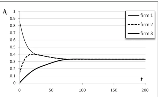
Fig. 3. Time series of the proportion of total scientists working in each nation in the standard scenario.

Fig. 3 shows that the distribution of the share of scientists working in each nation evolves very closely to that of the market shares. The essence of the convergence process shown in Figures 2 and 3 lies in the ability of emergent firm 3 to use its initial price advantage to sustain a process of gradual convergence in product performance. All along this process of technological catch-up, firm 3’s advantage in price is essential to sustain the level of competitiveness that enable firm 3 to gain market share steadily. Firm 3 manages to approach the (higher) product performance of its competitors because, all along the convergence process, firm 3’s R&D productivity is greater than its competitors’. This greater R&D productivity contributes to increase product performance directly, and also indirectly, by attracting mobile scientists. This is illustrated in Fig. 3, which shows that the share of total scientists working in firm 3 grows uninterruptedly.

19

sets lower prices than its rivals. For this reason, it starts to gain market share (see Fig. 2). However, this initial advantage regarding prices is not definitive for 3 reasons:

i) As firm3 gains market share, its price tends to approach that of its rivals –see (1). ii) Equations (12) and (13) show that a time will arrive when firm 3 will have to take

on debt. This fact will wear down the price advantage of the firm. We show in Fig. 4 how firm 3 increases its debt/capital ratio during the first part of the process.

Fig. 4. Time series of debt-to-capital ratios in the standard scenario.

According to (12) and (13), the reasons for firm 3 to take on debt are: firstly, the

intense growth rate of the sector g = 0.05; secondly, the high rate ₃3

s s

•

at which firm 3 initially gains market share –see Fig. 2; thirdly, the low initial profit of firm 3 –see Table 1 and (2); and, finally, firm 3’s increase in its R&D to profits ratio –see (10). iii)Despite the initial price advantage, we can see in Table 1 that firm 3 starts out from

) 0 ( ) 0 ( ) 0

( 2 1

3 x x

x < < . This disadvantage could have thwarted catch-up in Fig. 2, but firm 3 manages to improve its product to match the level of its rivals' –see (15).

20

(a) Regarding R&D productivity z3(t), it is greater than that of the other firms during the catch-up process (see the conditions in Table 1 for xi(0), Ti(0), λi).

(b) The proportion of scientists, h3(t) depends on both the national university systems and the international migration flows. In Table 1 it is clear that mobility is not high,

1 . 0

1−σ = , so the domestic University funding b3 =b1=b2 is important. However,

it is interesting to point out the evolution of immigration ratios

{

}

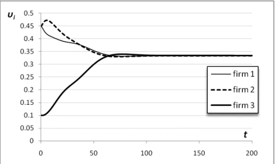
underlying Fig. 3. We show this evolution in Fig. 5.

Fig. 5. Time series of immigration ratios in the standard scenario.

Fig. 5 shows that the capacity of firm 3 to attract scientists becomes very significant. Equation (18) and Fig.1 help us to understand this result attending to the dynamics of zi(t) and wi(t). Thus, with (18) we know that the R&D productivity in the emergent firm acts as a non-monetary attractor of highly-skilled labor. Therefore, z3(t) explains, partly, the convergence in Fig. 3 and 5. Regarding salaries, the dynamics of {wi(t)

}

21

growth g. The increase in s3(t) in Fig. 2 favors the growth of salary w3(t) and, via this

effect, strengthens the increase in h₃(t) in Fig. 3. Finally, by comparing Figures 3 and 5,

we can see that the first stationary-state condition in section 3 is verified, so that h~i =υ~i.

To sum up, the analysis explained above allows us to list the following characteristics of the catch-up process generated from the standard scenario:

1) The emergent firm 3 enjoys an initial advantage in prices, which manages to transform into convergence in performance over the catch-up process.

2) For technological convergence to take place, it is essential that the emergent nation can count on support from science-related institutions giving it access to the worldwide technological frontier (Ti(t) common ∀i; see also the next section). 3) The previous characteristic means that firm 3 enjoys an advantage in R&D

productivity. At the same time, we have seen how this firm manages to transform this advantage into convergence in salaries over the process.

4) The convergence in salaries is possible thanks to the gradual increase in R&D spending by the emergent firm.

5) The effort made in educational expenditure by the emergent nation, together with its capacity to attract scientists, allow for a gradual rise in the share of scientists working in the emergent firm.

6) During the initial phase of the process, the emergent firm has to resort to debt to finance its intense growth. However, as the catch-up process advances, firm 3 manages to pay off its debt, thus avoiding insolvency.

4.3

Sensitivity analysis

22

performance of their products beyond their competitors’. This competitive edge allows them to capture a greater share of the market. As we will see, this advantage is so important that, in any stationary state, any difference in the technological frontier between two surviving firms with the same unit cost necessarily implies a persistent difference in their market shares (see appendix). In particular, a situation where all firms share the market equally can be stable only if the technological frontier is the same for all of them. Conversely, if all firms have a common technological frontier (like in the standard scenario), surviving firms end up dividing the market in equal shares. This statement, which is supported by the robustness analysis summarized in the next section, allows us to go deeper into the mechanisms that underlie the catch-up process.

More precisely, in order to understand the specific influences of Ti(0) and λi –the

parameters that shape the technological frontier of a firm–, let us define exij, the relative

edge in performance of firm i over firm j, as:

x x x

ex i j

ij

− =

And similarly, let esij be the relative edge in market-share of firm i over firm j, as:

s s s es i j

ij ₊

− =

1

We show in the appendix that in any stationary state, the following condition must hold between any two firms in the market with equal unit costs:

(

)

In particular, this condition reveals that in any stationary state, a greater product performance implies a greater market-share. And, as explained above, the greater the technological frontier is, the greater the performance. Here we focus on the role of Ti(0)

23

Fig. 6. Time series of firm 3’s market share for different values of T3(0).

Departing from the standard scenario, Fig. 6 shows the time series of firm 3’s market share for different values of T3(0). Clearly, a greater T3(0) implies a greater market share s3; it is also apparent that differences in Ti(0) do not preclude the perpetual coexistence of various

24

Fig. 7. Time series of firm 3’s market share for different values of T3(0) with α = 0.9.

The effect of λi is more fundamental, since differences in this parameter induce differences

in performance that can grow indefinitely. In particular, this means that –ceteris paribus– the surviving firm with the greatest λi will end up with the maximum edge in performance

exij over any other firm j. As an example, consider Fig 8, which shows the time series of

25

Fig. 8. Time series of market shares in the standard scenario with λ3 = 0.011.

Whether the absolute advantage in performance induced by having the greatest λi will

translate in complete dominance of the market or not, is a question that depends on the profile of the market demand (α). Drawing on the expressions of exij, and esij, it is

result and considering eq. (21), it can be shown that if

2

with the greatest λi will end up acquiring the whole market. Conversely, if

2

monopoly does not necessarily occur. Again, this key interaction between the technological frontier and market demand is illustrated in Fig. 9: the market must value low prices highly enough, to avoid a monopoly of the firm with the highest performance.

In the cases where 0.8

26 firms coexist.

Fig. 9. Time series of firm 3’s market share for different values of α, with λ3 = 0.02.

Having understood that differences in technological frontiers are responsible for persistent differences in market shares, we now turn to study the influence of the other parameters. These parameters do not have an impact on how surviving firms share the market in the long run, but they do influence a) which specific firms manage to survive, and b) how quickly surviving firms reach their long-run market-share. Regarding the former question, consider Table 2, which shows, for each parameter, the range of values within which the emergent firm 3 ends up approaching its stationary market share of 1/3, assuming the other parameters retain its value in the standard scenario. Table 2 shows that most changes in one parameter do not prevent the emergent firm from reaching its stationary share of 1/3. Thus, the result that firm 3 catches up is robust to changes in only one parameter at a time.

g A α β η χ σ ζ ε

(0,∞) (0,∞) [0.17,1) (0,1] [0,1] [0,1] [0,1] (0,∞) [0,1]

D3(0) K3(0) B3(0) b3 υ3(0) w3(0) x3(0) r3(0)

[0,38] (0,∞) (0,∞) (0,∞) (0,1] (0,∞) (0,∞) (0,1)

27

Regarding question b) above, we present in Table 3 the elasticity of the convergence time t3

with respect to various parameters.

g A α β η χ σ ζ ε λi Ti

0.136 -0.067 -1.683 0 -0.013 0.025 2.374 -0.054 -0.258 0.154 1.147

D3(0) K3(0) B3(0) b3 υ3(0) w3(0) x3(0) r3(0)

0.111 -0.404 -0.014 -0.087 -0.270 0.002 -1.313 -0.022

Table 3. Elasticity of t3 with respect to the parameters in the standard scenario. Elasticities have been

calculated computing the effect of a 10% change of each parameter on t3 (D3 was changed from 0 to 1).

The elasticity with respect to λi and Ti refer to simultaneous changes in all firms.

In Table 3, positive signs show that the larger the parametric value is, the larger t3 is.

Negative signs indicate that the larger the value of the considered parameter, the earlier the convergence process ends. The signs of the elasticities in Table 3 indicate that the process of convergence accelerates –that is to say, t3 is lower–, the higher the values of α ,ε and

3

b . Likewise, the positive sign of the elasticity of σshows that the higher the international mobility of scientists –that is, the higher (1–σ) is–, the lower t3 is. That is, the international

mobility of scientists, the price/performance sensitivity of demand, the sensitivity of scientists to non-monetary considerations and the budgetary effort of nation 3 act as pro-catch-up factors. On the other hand, the positive signs of the elasticities of g, χ _and D3(0) in

Table 3 show clearly that these parameters slow down the convergence process.

It is interesting to interpret some of the mechanisms which underlie the elasticities in Table 3. Thus, the negative elasticity of α reveals the pro-catch-up effect of this parameter. The reason is that the higher the value of α –the price/performance sensitivity of demand–, the more intensely the emergent firm can make the most of its initial advantage in prices. This means that firm 3 gains market share first, converges its R&D spending and salaries more quickly, and rapidly raises its share of scientists. The latter fact favors the convergence of the firm in performance and accelerates the process of catch-up.

28

of scientists to non-monetary factors. Its pro-catch-up character is explained by the fact that the higher the value of this parameter, the more scientists will be captured by the emergent nation, which makes the most of its initial attractiveness in questions of R&D productivity. This will accelerate the convergence in performance and catch-up.

Our attention is also drawn to the high intensity of the effects of σ (see Table 3). Clearly, the higher the international mobility of scientists (the higher 1–σ), the lower t3 is. This is so

because the emergent industry captures a greater volume of foreign scientists, making the most of its R&D productivity, and converges in performance with ease.

Finally, as we have seen, there are three factors which seem to delay significantly the catch-up process. The first one is g. Thus, the greater the growth rate of the sector, the more difficulties the emergent firm experiences in completing the catching-up. This is so as the emergent firm is obliged to take on more and more debt, the higher the growth rate experienced in the initial phase. This rate depends on g –see (8). The costs of this debt will wear down the initial advantage in prices, and the market share capture is delayed while the catch-up process is slowed down.

The other factors are χ and D3(0). To be specific, the higher the value of both parameters –

that is, the higher the initial level of debt in the emergent firm and the shorter the repayment period of the debt–, the greater the financial costs of firm 3. This wears down its initial advantage in prices and slows down the catch-up process.

4.4

Robustness Analysis

29

α 0 0.25 0.5 0.75 1

ε 0 0.25 0.5 0.75 1

σ 0 0.25 0.5 0.75 1

ζ 0.1 0.5 0.9 1

x3(0) 0.7 0.5 0.1

r3(0) 0.08 0.06 0.01

w3(0) 0.05 0.025 0.01

λi [0.005 0.005 0.005] [0.01 0.01 0.01] [0.05 0.05 0.05] Ki(0) [135 63 2] [130 60 10] [115 45 40]

Table 4. Definition of the parameter values used to conduct the robustness analysis. We have run the model for each possible combination of the parameter values shown in the table. This adds up to a total of 121500 simulation runs.

30

Fig. 10. Each pie chart summarises the result of 4860 simulation runs at time t = 1000. The value of α and ε in each pie chart is determined by its horizontal and vertical position respectively. The 4860 runs result from the 4860 combinations of the other parameter values, as indicated in Table 4. Within each pie chart, black represents the proportion of runs that ended up in monopoly, dark gray represents convergence of 2 firms, and light gray represents convergence of the 3 firms. White areas denote the proportion of runs that did not finish in any of these categories.

31

runs where the 3 firms converged by time t = 1000 for different values of α and ε in the whole simulation experiment (121500 runs).

Fig. 11. Proportion of runs where the 3 firms converged by time t = 1000 (i.e. convergence time t3 <

1000). Each column corresponds to 4860 simulation runs, giving a total of 121500 runs.

The three firms can converge also for low values of α and ε, but in those situations convergence becomes dependent on initial conditions and on other parameters, particularly on those that affect the process of technological catch-up. Thus, one of the most important parameters in such cases is the rate of global innovation. As an example, departing from the standard setting with α = 0.25 and ε = 0.25, it turns out that if λi = 0.05, monopoly prevails;

if λi = 0.01, we obtain duopoly; and if λi = 0.001, the three firms end up sharing the market

32

share, whilst this percentage rises up to 100% if x3(0) = 0.7 and λi = 0.005.

5

Concluding Remarks

We have proposed a model to analyze the sources of catch-up and leadership in science-based industries. The model shows how emergent firms can consolidate their position in a high-tech sector on the basis of innovation, competition and scientist mobility. Thus, departing from the standard scenario in Table 1, we have characterized a robust pattern of industrial up, and we have studied which parameters accelerate or slow down catch-up. The analysis has shown that, the price/performance sensitivity of demand, the sensitivity of scientists to non-monetary considerations, the degree of scientist mobility and the budgetary effort of the emergent nation accelerate catch-up. The factors which slow down the process are demand growth, the initial level of debt in the emergent firm, and the rate of debt amortization. The robustness analysis shows that such results are solid.

In addition, we have obtained some formal results which represent consistent regularities of the model. Thus, the stationary-state conditions presented in section 3 and 4.3 reveal the key role of the firms’ technological frontiers for industrial success. Furthermore, as we have seen, these stationary-state conditions highlight crucial interactions among technology-supporting institutions and market demand at the basis of industrial catch-up. The analysis in 4.4 confirms that our results are robust and points again to interesting interdependencies among innovation, scientist mobility and market demand.

6

Acknowledgements

33

Appendix

Statement 1: In any stationary situation with α∈

( )

( )

out of the market (i.e. si = 0) or, if they manage to hold a positive market share, then they present

the following relations among their variables: a) hi(t)=h~i =υi(t)=υ~i

Proof of 1a): In a stationary situation both the immigration ratios and the proportion of scientists

working in industry i must remain constant, i.e. h_i(t)=h~_i and υ_i(t)=υ~_i. Knowing that

Using equations (17) and (19):

(

)

And taking limits when t goes to infinity, we obtain that in a stationary situation the proportion of scientists working in industry i must equal the immigration ratio of that country in the long run, i.e.

i i

h~ =υ~.

Proof of 1b) and 1c): In a stationary situation the proportion of scientists working in industry i

must remain constant, i.e. hi(t)=h~i. Performance levels are driven by the differential equation:

(

)

As in Nelson and Phelps (1966), noting that h~_i >0we can solve these equations arriving at:

34

Therefore, in a stationary situation, in the long run:

,...,

and under these conditions the productivity of R&D remains constant and verifies:

,...,

Statement 2: In any stationary situation,any difference in the technological frontier between two

firms in the market with the same unit cost necessarily implies a persistent difference in their market shares.

Proof: Suppose that in the stationary situation, two firms i and j in the market have the same market

share, i.e. s_i =s_j >0, but i's technological frontier is greater than j’s, i.e. Ti >Tj.

> , and therefore the situation where

0

> = _j

i s

s cannot be stationary: firm i would increase its product performance more than firm j, and consequently, firm i would increase its market share beyond firm j.

Statement 3: In any stationary situation, the following condition must hold between any two firms

in the market with equal unit costs:

(

)

Proof: It is straightforward considering equal unit costs, (1), (3) and s i =0,∀i=1,...,n

•

35

References

Amsden, A. (2001). The Rise of the Rest. Challenges to the West from Late-Industrializing

Economies. Oxford University Press. New York.

Chiao, C. (2002). Relationship between Debt, R&D and Physical Investment. Evidence from US Firm-level Data. Applied Financial Economics, 12, 105-121.

Fatas-Villafranca, F. and Saura, D. (2004). Understanding the Demand-Side of Economic Change. A Contribution to Formal Evolutionary Theorizing. Economics of Innovation and New Technology,

13 (8), 695-716.

Fatas-Villafranca, F., Sanchez-Choliz, J. and Jarne, G. (2008). Modeling the Co-evolution of National Industries and Institutions. Industrial and Corporate Change, 17 (1), 65-108.

Fatas-Villafranca, F., Jarne, G. and Sanchez-Choliz, J. (2009). Industrial Leadership in Science Based Industries. A Co-evolution Model. Journal of Economic Behavior and Organization, 72 (1), 390-407.

Fatas-Villafranca, F., Saura, D. J., and Vázquez, F.J. (2009). Diversity, persistence and chaos in consumption patterns. Journal of Bioeconomics11, 43–63.

Hamilton, D. and Glain, S. (1995). Silicon Duel: Koreans Move to Grab Memory-Chip Market from the Japanese. The Wall Street Journal, March, 14, A1.

Khadria, B. (2004). Human Resources in Science and Technology in India and the International Mobility of Highly-Skilled Indians. OECD STI Working Paper 2004/07.

Malerba, F. (1985). The Semiconductor Business: The Economics of Rapid Growth and Decline. University of Wisconsin Press. Madison.

Malerba, F. (2006). Innovation and the Evolution of Industries. Journal of Evolutionary Economics,

16, 3-23.

Malerba, F., Nelson, R., Orsenigo, L. and Winter, S. (2008). Public Policies and Changing Boundaries of Firms in a "History-Friendly" Model of the co-evolution of the Computer and Semiconductor Industries. Journal of Economic Behavior and Organization, 67 (2), 355-380.

Mazzoleni, R. and Nelson, R.R. (2007). Public Research Institutions and Economic Catch-up.

Research Policy, 36, 1512-1528.

Metcalfe, J.S. (1998). Evolutionary Economics and Creative Destruction. Routledge. London.

Mowery, D.C. and Nelson, R.R. (1999) (eds) Sources of Industrial Leadership. Studies of Seven

Industries. Cambridge University Press. Cambridge, MA.

Murmann, J.P. (2003). Knowledge and Competitive Advantage. The co-evolution of Firms,

Technology and National Institutions. Cambridge University Press. Cambridge, MA.

Nelson, R.R. (2008). What Enables Rapid Economic Progress: What are the Needed Institutions.

36

Nelson, R.R. and Pack, H. (1999). The Asian Miracle and Modern Growth Theory. The Economic

Journal, 109, (July), 416-436.

Nelson, R.R. and Phelps, E.S. (1966). Investment in Humans, Technological Diffusion and Economic Growth. American Economic Review, 56, 69-75.

Nelson, R.R. and Wright, G. (1992). The Rise and Fall of American Technological Leadership: The Postwar Era in Historical Perspective. Journal of Economic Literature, December, 1931-1964..

Saxenian, A.L. (2006). The New Argonauts. Regional Advantage in a Global Economiy. Harvard University Press.

Silverberg, G. and Verspagen, B. (2005). Evolutionary Theorizing on Economic Growth. In Dopfer K. (ed) The Evolutionary Foundations of Economics. Cambridge University Press. Cambridge, UK.

Stiglitz, J.E. (1996). Some Lessons from the East Asian Miracle. The World Bank Research

Observer, 11 (2), 151-177.

Thorn, K. and Holm-Nielsen, L.B. (2006). International Mobility of Researchers and Scientists.

UNU-WIDER Research Paper, 83, 1-17.

37 List of symbols

n: number of firms/national industries. .

i

s : firm/Industry i’s market share.

i

p : firm i’s price.

i

c: firm i’s unit cost.

i

π : firm i’s unit profit.

i

x: firm i’s product performance.

α: price/performance sensitivity of demand.

i

γ : firm i’s level of competitiveness.

i

Q: firm i’s level of output.

i

K : firm i’s capital stock.

g: overall rate of demand growth.

A: capital productivity.

i

r: firm i’s R&D to profits ratio.

i

R : firm i’s R&D budget.

β: learning parameter.

η: rate of interest.

χ: debt amortization rate.

i

D : firm i’s stock of debt.

i

d : firm i’s debt to capital ratio.

i

θ: firm i’s financial needs indicator.

i

T: nation i’s technological frontier.

i

λ: expansion rate of the nation i’s technological frontier.

i

H : stock of scientists working in national industry i. (hi):share of total scientists.

i

w: salary of scientists in nation i.

i

z: R&D productivity in nation i.

i

y : number of scientists that finish their training at nation i at any time.

i

B : nation i’s university budget devoted to the relevant disciplines for the industry.

i

υ : immigration ratio.

ε: R&D productivity/wage sensitivity of scientists .