Self Similarity of Space Filling Curves
12
0
0
Texto completo
(2) Ingeniería y Competitividad, Volumen 18, No. 2, p. 113 - 124 (2016). 1. Introduction In 1878, Cantor established the equipotency between R and any n-dimensional euclidean space Rn (Sagan, 1994a). In the plane, it implies the existence of a bijective mapping from R to R2 (an interval can be mapped into the plane). A year later, Netto proved that such mapping cannot be continuous (Bader, 2013). A decade later, Peano proved the existence of a continuous surjective mapping from R to R2 (Sagan, 1994c). He proposed a continuous curve that goes through every point of the plane (Figure 1), and those curves were called Space Filling Curves (SFCs). SFCs has fascinated mathematicians since then, and brilliant mathematicians as Hilbert, Moore, Lebesgue, Meander, Poyla and Sierpinski has proposed their own SFCs exploring different properties and perspectives (Sagan, 1994a).. pattern recognition in several contexts (Rosenthal & Kouri, 1973; Lam & Liu, 1996). In the literature of Space Filling Curves, mathematicians have stated a close relation between SFCs and fractals. SFCs have patrons and regularities that also are commonly found in fractals and that relation has been linked to the self-similarity property of fractals (Plaza et al., 2005; Haverkort & Walderveen, 2010; Skubalska-Rafajowicz, 2005). Wunderlich (1954) linked fractals and SFCs by introducing Iterated Functions System (IFS) in the generation of discrete approximation of Space Filling Curves. IFS is a method to generate discrete approximation of fractals by means of their selfsimilarity property and recursive algorithms. In this way, a discrete approximation of a fractal of nth order is composed of a finite number of copies of itself that can only differ from the original in size and orientation and are integrated under a regular patron consistent through iterations. McClure (2003) studied the self-similarity of the Hilbert curve, and lays out the advantages derived from this property by utilizing Iterated Functions System (IFS) as Wunderlich (Hutchinson, 1981). But, since not all SFCs are exact self-similar, in this paper, we propose a method to determine whether a discrete approximation of Space Filling Curve is exact self-similar.. Figure 1. A discrete approximation of the Peano Space Filling Curve.. But mathematicians are not the only ones who have been fascinated with SFCs, they also are extensively used in engineering (Bader, 2013). SFCs are used to solve combinatorial optimization problems in industrial contexts (Hu & Wang, 2004; Hua & Zhou, 2008). They also have been used as a scanning technique for image processing and compression (Dafner et al., 2000). Anotaipaiboom & Makhanov (2005) used SFCs to plan movement paths of robotic arms with numeric control. Additionally, Valle & Ortiz (2011), Bahi et al. (2008), and Chen & Chang (2005) have explored applications of SFCs for clustering. Furthermore, SFCs have been used for. 114. Despite the extensive attention that SFCs have received in the literature and their evident link with fractals, there is no formal definition for their self-similarity. This paper presents a formal conceptualization of the self-similarity adapted to the context SFCs and an efficient computational test to determine whether a specific SFC is self-similar. The paper is organized as follows: Section 2 presents an introduction to the theory of selfsimilarity and to SFCs theory, also a definition of exact self-similarity of discrete approximations of SFC. Section 3 presents the test that determine whether a discrete approximation of a Space Filling Curve on the plane is exact self-similar. In Section 4, we determine self-similarity of four.
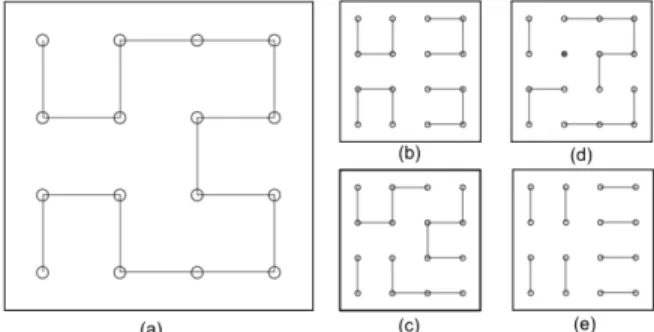
(3) Ingeniería y Competitividad, Volumen 18, No. 2, p. 113 - 124 (2016). of the most representative SFCs using our test. Finally, Section 5 provides conclusions and future research. 2. Context By definition, every fractal has the property of selfsimilarity (Barnsley, 1993). A set is self-similar if when we examine small portions of it, we only see reproductions of our initial set (Rubiano, 2002), as shown in Figure 2.. as in geometry a triangle is represented by three non-collinear points, we represent a SFC by means of an ordered finite list of points, SFC = {p1,p2,……,pn}. Figure 3a shows the Hilbert curve and the circles indicate the set of points by which it is represented. In this case, the Hilbert curve is found in the 4x4 lattice, hence 16 points are used to represent it. The order in which these points are found in the list, is the same order in which these points are found in the curve. Figures 3b, 3c, 3d and 3e show partitions of the curve of Figure 3a. Figure 3b is a partition with four equivalence classes, and each equivalence class has four points. Note that the union of the four equivalence classes equals the 16 points in Figure 3a and no point belongs to more than one equivalence class.. Figure 2. Sierpinski triangle.. Ferrari (2007) establishes a formal definition of self-similarity, as follows: Definition 1: ∩. A compact set X R2 is self-similar if there is a finite set of contractive similarities FN ={F1,F2,…Fn} such n that X= i=1 Fi (X) and the subsets of X of the form Fi (X) overlap only in the boundaries.. Figure 3. Different cardinality partitions of Hilbert curve.. ∩. Contractive similarities are affine transformations of the form Fi = ri Di x+bi, where ri is a scalar such that 0< ri < 1, Di is the matrix of rotations and bi is n a vector in R2 (Barnsley 1993). Note that i=1 Fi (X) is a cover of X. In addition, the intersection of subsets Fi (X) is only allowed on the borders, a property which makes it a quasi-partition. In SFCs context, the latter restriction is even stronger, since these curves go through every point of the n plane exactly once. Thus, in SFCs context, i=1 Fi (X) is a partition of X and every Fi (X) is an equivalence class.. 3. Self-Similarity Test It is seen in Figure 2 that the largest triangle is made up of three smaller triangles which in turn are made up of three smaller ones. To prove selfsimilarity of this set, it is sufficient to show its IFS, which is easily found by inspection. However, it is not always evident to prove self-similarity of a set. According to the definition of self-similarity, in order to prove that a set is not self-similar, it is necessary to show the non-existence of a partition such that all equivalence classes pi of be contractive similarities of X, that is,. ∩. ∩. In this paper, we analyze SFCs from a combinatorial point of view, just as Dai & Su (2003) do. As well. 115.
(4) Ingeniería y Competitividad, Volumen 18, No. 2, p. 113 - 124 (2016). Thus the formula may be written as,. This would imply that to prove the self-similarity of a compact set X, it is necessary to evaluate all partitions of X and find in everyone of them an equivalence class which is not an affine transformation of X. This is a very expensive computational task, mainly because the amount of partitions of X is very large (Rota 1964).. of partitions included in H until the only one left is CM. The basic foundations for the process are the following two propositions: Proposition 1: It is necessary that all equivalence be affine transformations of X, classes pi of for X to be self-similar under . Proposition 2: It is necessary that all equivalence classes pi of be affine transformations of each other, for X to be self-similar under .. In this paper, we present a self-similarity test that is useful to determine whether a SFC is self-similar or not. For a given curve X, the test identifies a special partition of X that we denote CM, such that X is self-similar if and only if X is self-similar under CM. Lastly, it determines if X is self-similar under CM, or not. It is thus necessary to prove self-similarity of X under one partition only, which substantially lowers the computational cost.. Proposition 1 follows from Definition 1. For proposition 2, it has to be shown that:. The reader will next find section 3.1 where the procedure to identify the CM partition of X is described, and section 3.2 where it is shown how to determine the self-similarity of X under a partition .. If X is self-similar under , then, according to Definition 1, each equivalence class of pi of is a contractive similarity of X. That is,. Let the reader be reminded that the procedures and propositions from here on must be considered in the context of the SFCs and do not apply directly to every type of set.. Ferrari (2007) shows that all contractive similarities are invertible and their inverse functions are also affine transformations. Let’s call Wj the inverse function of Fj. Thus, we say that,. If X is self-similar under , then, Where pi is the equivalence class i of and G is an affine transformation. In this case, is a necessary condition for X to be self-similar under .. 3.1 CM Partition of X Equivalently, it’s stated that,. ∩. Let’s call P(X) the set of all partitions of X. Since CM P(X), what we will do to find CM is to progressively eliminate all partitions of P(X) under which we know beforehand that X is not self-similar. To do this, we will resort to the properties of selfsimilar sets, in such manner that each property will help us discard those partitions of P(X) that do not comply with it. Let’s denote by H the subset of P(X) in which we consider that CM is found. We start by equating H to P(X), and then, by applying each property we will gradually reduce the amount. 116. Let’s call Fk the contractive similarity, such that equivalence class pk equals Fk (X). Next, transformation Fk is applied to both sides of the previous equation and we get that,. Finally, let’s call G the composition of Fk and Wj, G=Fk ◦Wj, assuring that G is also an affine transformation, as it is a composition of two affine transformations, thus getting,.
(5) Ingeniería y Competitividad, Volumen 18, No. 2, p. 113 - 124 (2016). Equivalently, we say that,. This way, we have shown in this manner that for a compact set to be self-similar under it is necessary that all equivalence classes of be affine transformations of one another, in pairs. It is inferred from Proposition 2 that Η should only contain partitions in which all equivalence classes be affine in pairs. Notice now that when applying an affine transformation to any curve (ordered set of points) the amount of points on the curve (cardinality) will always be conserved. This means that , where S is a curve, F is an affine transformation and #(S), #(F(S)) are the corresponding cardinalities of S and F(S). By doing this, we assert that if two curves do not have the same cardinality, then one is not an affine transformation of the other and vice versa. From this assertion we derive Criterion 1. Criterion 1: We include in H only those partitions in which all equivalence classes have the same cardinality. This cardinality we shall call n. Figure 3a shows a sixteen-point approximation of the Hilbert curve. Different examples of partitions of this curve are shown in Figures 3b, 3c, 3d and 3e. Of the four partitions shown, Figures 3b and 3e comply with Criterion 1 with n=4 and n=2 respectively. Figures 3c and 3d do not comply with criterion 1 since their equivalence classes have different number of points. Note that it is necessary that all equivalence classes pi of a partition be contractive similarities of X, for X to be self-similar under (Definition 1). Since the contractive similarities do not alter the amount of elements of the original set, the cardinality of X under and that of each equivalence class must also be guaranteed to be equal. Let’s denote by m the cardinality of X under , which is the number of equivalence classes of . From this we derive Criterion 2.. Criterion 2: We include in Η only those partitions whose equivalence classes have the same cardinality of X under . The partition in Figure 3e does not satisfy Criterion 2 because it has eight equivalent classes, that is, m = 8 and its equivalence classes have 2 points each, i.e., n =2. The partition in Figure 3e does not satisfy Criterion 2 because it has eight equivalent classes, that is, m=8 and its equivalence classes have 2 points each, i.e., n =2. According with the above assertions, one concludes that H only contains partitions whose equivalence classes have the same cardinality, and in addition, that this cardinality must be equal to the number of equivalence classes, that is, n = m. Note now that the amount of points of a curve X, divided by the number of equivalence classes equals the number of points of each equivalence class, that is, #(X)/m = n. Replacing n = m, we get #(X) = n2; from which Criterion 3 is derived. Criterion 3: We include in H only those partitions whose equivalence classes are equal to the cardinality of each equivalence class that is equal in turn to the square root of the cardinality of curve X. This means that for a sixteen-point curve, only those partitions which have four equivalence classes are useful, where each equivalence class in turn has four points (Figure 3b). So far, H includes all partitions that satisfy criteria 1, 2 and 3. This is considering all partitions of X with n equivalence classes and each equivalence class with n points, i.e., the number of partitions of X included in H equals all possible combinations of the number of points of X in n subsets (combinatorial number). We will now resort to the arc-connectedness property to clean out set H. Figure 4 shows four partitions of the Hilbert curve. Each partition has four equivalence classes and each equivalence class contains four points. Figure 4d shows two equivalence classes that. 117.
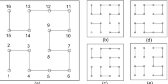
(6) Ingeniería y Competitividad, Volumen 18, No. 2, p. 113 - 124 (2016). are arc-connected and two equivalence classes that are not arc connected. On the other hand, Figure 4e shows one arc-connected equivalence class and three equivalence classes that are not arc-connected. Note that affine transformations do not affect a curve’s arc-connectedness. Thus, the arcconnected equivalence class of Figure 4e cannot be transformed by means of an affine transformation to any of the other equivalence classes of this partition. It is therefore excluded from H, according to Proposition 2. We state that in general, if a partition has a non-arc-connected equivalence class, then is not included in H. Criterion 4 is derived from this. Criterion 4: We include in Η only those partitions whose equivalence classes are arcconnected sets.. The partition in Figure 5d contains two equivalence classes and each equivalence class contains eight points. The reader, by direct inspection, can verify that this is the only way to divide the curve of Figure 5a in two parts with the same number of points and that each part is arc-connected. Proposition 3 is derived from this. Proposition 3: If there is a partition of a curve X with m equivalence classes, such that each equivalence class is arcconnected and has n number of points, then that partition is unique. Sagan (Space-Filling Curves, 1994) defines an SFC as a continuous curve with a positive Jordan content. In this context, a continuous curve is a connected and locally connected compact curve (Sagan 1994: Space-Filling Curves, Chapter 1, Introduction). Bing (1952) states that every continuous curve is a continuous transformation of an interval of a straight line. This leads us to conclude that SFCs are continuous transformations of a segment of a straight line and thus establish a relation of equivalence between them (Figure 6).. Figure 4. Non-arc-connected partitions of Hilbert curve. In Figure 5, there are four partitions of the Hilbert curve all of whose equivalence classes are arc-connected sets. The numbers in Figure 5a indicate the order in which are found the points located on the curve.. Figure 5. Connected partitions of Hilbert curve. 118. Figure 6. Equivalence of a SFC with a straight line interval.. Finally, we can use the theorem of unique segments (Bing 1952) to establish the existence of a unique equi-partition of the straight line interval to conclude that the partition is unique as proposition 3 states. From a discrete point of view, this means that there is only one way in which the straight line interval of Figure 6 can be divided into four parts with the same number of points. Now, we integrate Criterion 3, Criterion 4 and Proposition 3. Criterion 3 indicates that in H we will.
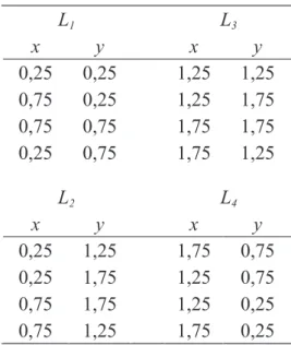
(7) Ingeniería y Competitividad, Volumen 18, No. 2, p. 113 - 124 (2016). only include those partitions of X such that n=m= √(#(X). Criterion 4 says that of these partitions, only are considered those whose equivalence classes are arc-connected. Lastly, Proposition 3 states that if there is a partition of X satisfying both Criterion 3 and Criterion 4, then that partition is unique. CM Partition of the Hilbert curve (Figure 3a) is shown in Figure 3b.. Table 1: List of points of curve in Figure 3a.. x 0,25 0,75 0,75 0,25 0,25 0,25 0,75 0,75 1,25 1,25 1,75 1,75 1,75 1,25 1,25 1,75. Definition 2: Partition CM of curve X is a partition of X that satisfies the following conditions: it has n equivalence classes, each equivalence class has n points, and each equivalence class is an arcconnected set. In addition, if CM exists, then it is unique. The following is an algorithm to find partition CM of a given curve. Algorithm 1 Input: X, curve represented by an ordered list of points.. y 0,25 0,25 0,75 0,75 1,25 1,75 1,75 1,25 1,25 1,75 1,75 1,25 0,75 0,75 0,25 0,25. The CM partition of this curve, Figure 3b, is composed of 4 equivalence classes, i.e., n=4 in this case. The function splitList divides a list in n parts with equal number of elements and yields a list of lists of points. According to this, CM={L1,L2,L3,L4 }, where: Table 2: List of points of partition in Figure 3b.. Output: CM, structure storing ordered lists of points. procedure CMpartition (X) { n ← √(length(X) CM ← splitList(X, n) return CM } Let’s consider the example of Figures 3a and 3b. The curve in Figure 3a could be represented by the list of points in Table 1.. x 0,25 0,75 0,75 0,25 x 0,25 0,25 0,75 0,75. L1. L2. y 0,25 0,25 0,75 0,75 y 1,25 1,75 1,75 1,25. x 1,25 1,25 1,75 1,75 x 1,75 1,25 1,25 1,75. L3. L4. y 1,25 1,75 1,75 1,25 y 0,75 0,75 0,25 0,25. 119.
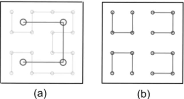
(8) Ingeniería y Competitividad, Volumen 18, No. 2, p. 113 - 124 (2016). 3.2 Self-SimilarityTest of X under Once CM partition is identified, we verify if X is self-similar under this partition. Remember that X is self-similar if and only if it is self-similar under CM. To determine self-similarity of X and a partition , we will prove that each equivalence class of is an affine transformation of X. If all equivalence classes of are affine transformations of X, then X is self-similar under . We say that X is not self-similar under in case that any equivalence class of is not an affine transformation of X. To determine if X is an affine transformation of an equivalence class pi of , we need to review the concept of scale invariance. Note that there is not any affine transformation that transforms the Hilbert curve, Figure 3a, in any of the equivalence classes of Figure 3b. This does not mean though that Hilbert curve is not self-similar. X should not be considered in this case as being the original curve, but as partition . By doing this, X is understood as a set of equivalence classes and it is thus that it must be compared with each equivalence class pi. Figure 7b shows the CM partition of the Hilbert curve, composed of four equivalence classes of four points each. Figure 7a shows Hilbert curve considered as a set of equivalence classes of the partition shown in Figure 7b. To determine whether the Hilbert curve is self-similar or not, we must prove that each of the four equivalence classes in Figure 7b is an affine transformation of the highlighted curve in Figure 7a. Given two curves X and Y, X will be an affine transformation of Y if and only if there is a matrix D and a vector b such that (Definition 1), where i is the point i of curve Y and i is the point i of curve X. To find D and b we can use a system of equations with six variables (D2×2,b2×1) and k equations, where k is the number of points of the curves. If the system has a solution, then X is an affine transformation of Y. If it does not have a solution, then X is not an affine transformation of Y. Another way to do it is by choosing three noncollinear points and finding the affine transformation. 120. transformation F which transforms these points of X in into the corresponding ones in Y. It is known that F exists and is unique for these three points. We find F(X) and state that X is an affine transformation of Y if and only if F(X)=Y.. Figure 7. Self-Similarity of a curve under a partition. Algorithm 2: Evaluate self-similarity of a curve X under a partition Input: , partition of curve X, represented by a list of lists of points. Output: bool, boolean indicating whether X is or is not self-similar under . procedure selfsimilarityXunderP ( ) { Xscale← ScaleP( ) bool← AT(Xscale, ) return bool } Let’s take the example in Figure 7a. Curve X is described in Table 1. Partition ={L1,L2,L3,L4 } of Figure 7b is found in Table 2. The first step in the algorithm scales X, ScaleP( ), as shown in Figure 7a. Xscale is thus represented by: Table 3. Xscale de la Figure 7a.. x 0,5 0,5 1,5 1,5. y 0,5 1,5 1,5 0,5.
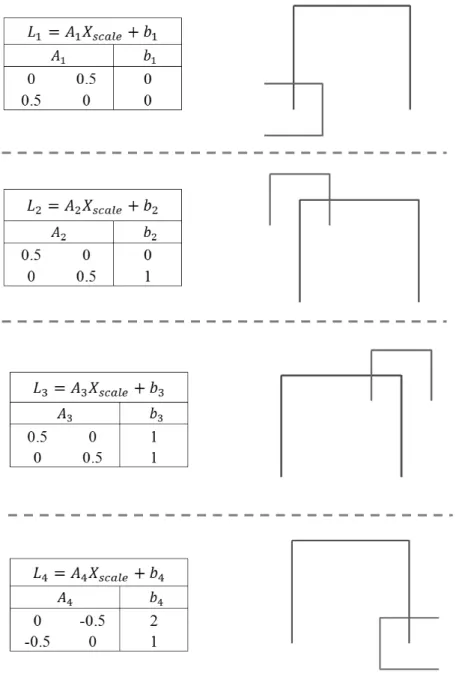
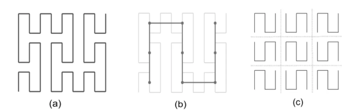
(9) Ingeniería y Competitividad, Volumen 18, No. 2, p. 113 - 124 (2016). The second step in the algorithm, AT(Xscale, ), evaluates whether Xscale is an affine transformation of all equivalence classes of . Figure 8 shows the affine transformation in matrix notation so that. Li=Ai Xscale+bi. Since all equivalence classes are affine transformations of X it is then said that X is self-similar under and, as a result, X is a selfsimilar curve.. Figure 8: Affine transformations of Xscale. 4. Applications We will show in this section four applications of the self-similarity test. In order to do that, we will utilize Peano, Moore, Meander and Lebesgue curves, presented in (Sagan, 1994).. Figure 9a shows the Peano curve. Figure 9b shows Xscale of Peano curve using the CM partition. And CM partition is shown in Figure 9c, which was found using Algorithm 1. The same procedure is followed in Figures 10, 11 and 12.. 121.
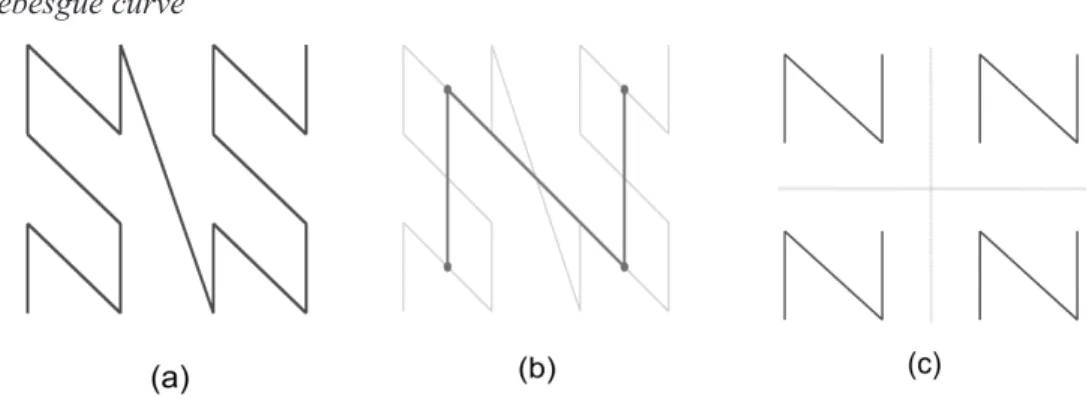
(10) Ingeniería y Competitividad, Volumen 18, No. 2, p. 113 - 124 (2016). To determine the self-similarity of each curve, we verify that Xscale is an affine transformation of each equivalence class of CM partition. To do this, we used the test of Algorithm 2 for each curve under the CM partition found with Algorithm 1. We found that Peano curve is self-similar, Moore curve is not self-similar, Meander curve is self-. similar and Lebesgue curve is self-similar. This result is congruent with what we observed in Figures 9, 10, 11 and 12. Note that in Figures 9, 11 and 12, all equivalence classes of partition CM are affine transformations of Xscale, while in Figure 10, Xscale is not an affine transformation of any equivalence class of CM partition.. Peano curve. Figure 9. Self-Similarity Test for Peano curve.. Moore curve. Figure 10. Self-Similarity Test for Moore curve.. Meander curve. Figure 11. Self-Similarity Tests for Meander curve.. 122.
(11) Ingeniería y Competitividad, Volumen 18, No. 2, p. 113 - 124 (2016). Lebesgue curve. Figure 12. Self-Similarity Test for Lebesgue curve.. 5. Conclusions and Further Research In this paper, we developed a test to determine self-similarity of an SFC and applied it to determine the self-similarity of four famous SFCs. In addition, we introduced several propositions and properties relating SFCs, selfsimilarity and affine transformations. These postulates can be used as a basis to formalize a theoretical structure of SFCs self-similarity. We established necessary and sufficient conditions for SFC self-similarity. This allows an extension of the work of McClure (2003). For further research, we suggest to use iterated systems of functions, both for generation of SFCs as for their application in different engineering fields. We also recommend to further study SFC self similarity for less restrictive self-similarities, such as statistical self-similarity. This would permit the growth of applications in the fields of image processing and pattern recognition. 6. References Anotaipaiboom, W. & Makhanov, S. (2005). Tool path generation for five-axis NC machining using adaptive space-filling curves. International Journal of Production Research 8 (15), 1643-1665. Bader, M. (2013). Space-Filling Curves. Heidelberg: Springer Berlin Heidelberg. Bahi, J. M., Makhoul, A. & Mostefaoui, A. (2008) Hilbert mobile beacon for localization and coverage. in sensor networks. International Journal of Systems Science 39 (11), 1081-1094. Barnsley, M. (1993). Fractals everywhere. San Diego, CA: Morgan Kaufmann Publishers. Bing, R.H. (1952). Partitioning continuous curves. Bull. Amer. Math. Soc. 58 (5), 536-556. Chen, H.-L. y Chang, Y.-I., Neighbor-finding based on space-filing curves, Information Systems, 30 (2005), 205-226. Dafner, R., Cohen, D. & Matias, Y. (2000). Context-based Space Filling Curves. Computer Graphics Forum 19 (3), 209-219. Dai, H. & Su, H. (2003). On the Locality Properties of Space-Filling Curves. Algorithms and Computation: 14th International Symposium, ISAAC 2003, Proceedings, Kyoto, Japan, p. 385-394. Ferrari, M. (2007). The convex Hull of SelfSimilar sets in R3. Fractals 15 (2), 197–206. Haverkort, H. & van Walderveen, F. (2010) Locality and bounding-box quality of twodimensional space-filling curves. Computational Geometry 43 (2), 131-147. Hu, M.H. & Wang, M.J. (2004). Using genetic algorithms on facilities layout problems. Int J Adv Manuf Technol 23 (3), 301–310.. 123.
(12) Ingeniería y Competitividad, Volumen 18, No. 2, p. 113 - 124 (2016). Hua, W. & Zhou, C. (2008). Clusters and fillingcurve-based storage assignment in a circuit board assembly kitting area. IIE Transactions 40 (6), 569–585. Hutchinson, J. (1981). Fractals and self-similarity. Indiana University Mathematics Journal 30 (5), 713-747. Lam, N. S.-N. & Liu, K.b. (1996) Use of spacefilling curves in generating a national rural sampling frame for hiv/aids research. The Professional Geographer 48 (3), 321-332. McClure, M. (2003). Self-similar structure in Hilbert's space-filling curve. Mathematics magazine 76 (1), 40-47. Plaza, A., Surez, J. & Padrn, M. (2005) Fractality of refined triangular grids and space-filling curves. Engineering with Computing 20 (4), 323-332. Rosenthal, C.M. & Kouri, D.J. (1973) Scattering amplitudes calculated with continuous spacefilling curves. Molecular Physics 26 (3), 549-560. Rota, G.C. (1964). The Number of Partitions of a Set. American Mathematical Monthly 71 (5), 498-504.. Rubiano, G. (2002). Fractales para profanos. Bogotá: UNIBIBLOS. Sagan, H. (1994a). Space-Filling Curves. Nueva York: Springer-Verlag. Sagan, H. (1994b). Introduction. In: H. Sagan, Space-Filling Curves. Nueva-York: SpringerVerlag. (Chapter 1). Sagan, H. (1994c). Peano's space filling curve. In: H. Sagan, Space-Filling Curves. Nueva-York: Springer-Verlag. (Chapter 3). Skubalska-Rafajowicz, E. (2005) A new method of estimation of the box-counting dimension of multivariate objects using space-filling curves. Nonlinear Analysis: Theory, Methods & Apps. 63 (5-7), 1281-1287. Valle, Y. & Ortiz, J. (2011) An efficient representation of quadtrees and bintrees for multi resolution terrain models. Geo-spatial Information Science 14 (3), 198-206. Wunderlich, W. (1954) Irregular curves and functional equations. Proceedings of the Benares Mathematical Society 5, 215-230.. Revista Ingeniería y Competitividad por Universidad del Valle se encuentra bajo una licencia Creative Commons Reconocimiento - Debe reconocer adecuadamente la autoría, proporcionar un enlace a la licencia e indicar si se han realizado cambios. Puede hacerlo de cualquier manera razonable, pero no de una manera que sugiera que tiene el apoyo del licenciador o lo recibe por el uso que hace.. 124.
(13)
Figure
+4
Documento similar
We recall that M ¯ g,n is an irreducible projective variety whose points correspond bijectively to the set of isomorphism classes of stable curves (or, equivalently, Riemann
The main aim of this work is to develop a consistent theory to determine the self-gravitational potential at an arbitrary point of each component of a detached close binary system in
In the literature there is an absence of research data on a persons movement in his or her own house that is not biased by self-report or by third party observation. We are in
Jones’s proof of the “if” direction of Theorem 1.1 is an intricate “farthest insertion” construction of a curve containing K, together with an amortized analysis showing that
The curve X is said to be a Q-curve if it is isogenous to all Galois conjugates. Firstly, we consider the rational points provided by Magma. In §4, we show how the j-invariants of
The main tool used is the decomposition of any rectifiable closed curve in a sequence of Jordan curves plus some curves with null index functions and an exceptional set.. 1
No obstante, como esta enfermedad afecta a cada persona de manera diferente, no todas las opciones de cuidado y tratamiento pueden ser apropiadas para cada individuo.. La forma
The Dwellers in the Garden of Allah 109... The Dwellers in the Garden of Allah
