Relationship between physical and acoustical parameters for road surface characterization

Texto completo

(1)Instituto Tecnológico y de Estudios Superiores de Monterrey Campus Monterrey. School of Engineering and Sciences. Relationship between physical and acoustical parameters for road surface characterization A thesis presented by. Jesús Rodrigo Leos Suárez Submitted to the School of Engineering and Sciences in partial fulfillment of the requirements for the degree of Master of Science In Manufacturing Systems. Monterrey, Nuevo León, December 04th, 2018.

(2)

(3) iii.

(4) @2018 by Jesús Rodrigo Leos Suárez All rights reserved.

(5) Dedication To God, for allowing me to reach this stage of my life and give me the courage to keep going. To my family, who taught me that roads are formed, that life is not easy, but that there are always solutions. That fate is not expected but reached. To you who formed me with love, repeating with hugs that I could be, who I wanted to be, that I could achieve everything, if I make an effort to do so. To you who taught me to enjoy the present, but to look forward to the future. That a failure, it is just a new opportunity to start over. To you, who with your experience, support, understanding and dedication, plant in me the healthy ambition to achieve this goal, which ends today. To you all, THANK YOU.. v.

(6) Acknowledgements I would like to express my deepest gratitude to Dr. David Ibarra for all his dedication and orientation, but specially for his friendship. To my family, for their continuous motivation and support through all the process to make this and all my goals possible. To my best friends Iván Vázquez, Gerardo Maycotte, Daniel Rimada and Mauricio Pérez, with great admiration to you all. To my fellow students and friends Oscar Jesús Escalera, José Alberto Robles, Javier Sierra, Sergio Alahudy, Jorge Islas, Pedro Vázquez, José Luis Padilla and Alan Pérez for all being part of a supporting group with the best hopes even at difficult times. The project in collaboration with the Institute for Automotive Engineering in Aachen (IKA), but specially to M. Sc. Christian Carrillo for giving me the opportunity to work together in mutual projects and gaining experience from very interesting automotive research projects. And finally, I want to thank Tecnológico de Monterrey for the current support tuition, with almost 10 years of my life studying at this great institution, and CONACYT for the maintenance support during the last 2 years..

(7) v.

(8) Relationship between physical and acoustical parameters for road surface characterization By Jesús Rodrigo Leos Suárez. Abstract An acoustic system for automated road surface conditions detection from acoustic signals of surface interaction is introduced. The aim of this work is to obtain different characteristics of the roadway surface by which the vehicle is circulating, to analyze its texture, friction and other characteristics related to the road surface with anticipation so that this information could be used in future automotive safety applications. The advantages of using an acoustic device compared with other current technologies is the low cost of the equipment and its portability. The robustness of our approach is evaluated on audio that span an extensive range of vehicle speeds, noises from the environment, road surface types, and pavement conditions including international friction index (IFI) values from 0 km/hr to 100 km/hr. The training and evaluation of the model were performed on different roads to minimize the impact of environment and other external factors on the accuracy of the classification. The results showed that there is a correlation between what we measured with the mechanical systems and what we obtained as a reply from the acoustic system. The hypothesis is that with the application of an acoustic device that characterizes the pavement in real time, future automotive applications such as adjusting the ABS system automatically in an optimal range of braking, showing a warning indicator light on the dashboard, or improving the driving decision making of autonomous cars will be possible by having prior information of the slippery surface conditions in which the vehicle transits..

(9) List of Figures Figure 1 - Passenger vehicle with all-season tires: Approximate stopping distance in meters. Modified from [7] ............................................................................................ 2 Figure 2 - Typical conformation of a flexible pavement. ............................................ 8 Figure 3 - Typical conformation of a rigid pavement. ................................................. 8 Figure 4 - Schematic Plot of Hysteresis and Adhesion .............................................. 10 Figure 5 - Influence of the range of surface irregularities in the phenomena of interaction between vehicles and the road. [12] ......................................................... 12 Figure 6 – Example of equipment used to characterize asphalt ................................. 13 Figure 7 - British friction pendulum (ASTM E 274) ................................................. 14 Figure 8 – Schematic of British Pendulum tester....................................................... 15 Figure 9 – Sand patch test (ASTM E 965) ................................................................. 17 Figure 10 - Interpretation areas of the diagram Friction vs. Macrotexture [15] ........ 21 Figure 11 - Wave vector K0 incident to a surface containing cylinders of radius a and mean center-to-center spacing b [37]. ........................................................................ 22 Figure 12 - Wave vector K0 incident to a rough surface ξ ........................................ 23 Figure 13 - Geometry to study the attenuation between source and receiver in presence of a porous ground formed with several absorbent layers .......................... 24 Figure 14 - A plane wave incident on a homogeneous medium. ............................... 26 Figure 15 - Experimental setup. ................................................................................. 27 Figure 16- Experimental difference curves at different speeds with noise filtered. .. 28 Figure 17- Theoretical and experimental level difference curves for the asphalt at 100 km/h. ........................................................................................................................... 29 Figure 18 - Comparison chart of flow resistivity, porosity and shape factor at 0 and 100 km/h ..................................................................................................................... 30 Figure 19– Location of measurements around the ITESM – Campus Monterrey ..... 31 Figure 20 – Friction measurement at 1st location ....................................................... 32 Figure 21– Macrotexture measurement at 3th location.............................................. 33 Figure 22 - Comparison of sections with IFI (F60, Sp) ............................................. 34 Figure 23 – Acceptance/Rejection curve for the five locations ................................. 35 Figure 24 – Static system ........................................................................................... 37 Figure 25 – Acoustic measurement at the 1st location ............................................... 37 Figure 26 - Comparison of flow resistivity for 1 to 4 parameters .............................. 39 Figure 27 - Comparison of porosity for 3 and 4 parameters ...................................... 39 Figure 28 - Comparison of tortuosity for 3 and 4 parameters .................................... 39 Figure 29- Representation of the acoustic system mounted on the car ...................... 40 Figure 30 - Acoustic system mounted at the front of the driver’s rear tire ................ 40 Figure 31 - Comparison of flow resistivity for 1 to 4 parameters .............................. 42 ix.

(10) Figure 32 - Comparison of porosity for 3 and 4 parameters ...................................... 42 Figure 33 - Comparison of tortuosity for 3 and 4 parameters .................................... 42 Figure 34 - Correlation between IFI and Porosity with 3 parameters. (r=0.26) ........ 44 Figure 35 - Correlation between IFI and Porosity with 4 parameters. (r=0.25) ........ 44 Figure 36 - Correlation between IFI and Porosity with 3 parameters (r=-0.85) ........ 45 Figure 37 - Correlation between IFI and Porosity with 4 parameters (r=-0.27) ........ 45 Figure 38 - Correlation between Friction and Porosity with 3 parameters (r=-0.42) 46 Figure 39 - Correlation between Friction and Porosity with 4 parameters (r=-0.5) .. 46 Figure 40 - ABS System. ............................................................................................ 49 Figure 41 - Braking slip effect on friction coefficient vs. wheel slip ........................ 49 Figure 42 - Work flow of the implementation. .......................................................... 50 Figure 43 – Elements of an Anti-Lock Braking System (ABS) model ..................... 50 Figure 44 – Slippery Condition Warning ................................................................... 51 Figure 45– Automated driving system ....................................................................... 51 Figure 46 - Correction factor for temperature. ........................................................... 60 Figure 47 - Matlab Graphical User Interface (GUI) .................................................. 63 Figure 48 – Theoretical and experimental level difference curves for the asphalt at 20 km/h ............................................................................................................................ 64 Figure 49 - Theoretical and experimental level difference curves for the asphalt at 100 km/h ..................................................................................................................... 65 Figure 50 - Layer of fluid. .......................................................................................... 68 Figure 51 - Layer of fluid backed by a rigid wall ...................................................... 69 Figure 52 – Sample tests divided by percentage of asphalt 76-22. ............................ 72 Figure 53 - British pendulum measurement experimentation .................................... 73 Figure 54 – Analysis of measurements using MATLAB........................................... 73 Figure 55 – Acoustic absorption comparison between 700-1100 Hz ........................ 74 Figure 56 – Friction vs Ac. Absorption for 700 Hz ................................................... 75 Figure 57 – Friction vs Ac. Absorption for 800 Hz ................................................... 75 Figure 58– Friction vs Ac. Absorption for 900 Hz .................................................... 76 Figure 59 – Friction vs Ac. Absorption for 1000 Hz ................................................. 76 Figure 60 – Friction vs Ac. Absorption for 1100 Hz ................................................. 76 Figure 61 - Impedance tube configuration I: microphone A in position 1 and microphone B in position 2. ....................................................................................... 79 Figure 62 - Impedance tube configuration II: microphone B in position 1 and microphone A in position 2. ....................................................................................... 79 Figure 63 – Example of microphone assembly. [49] ................................................. 81 Figure 64 – Example of system assembly. [49] ......................................................... 81.

(11) List of Tables Table 1 – Factors affecting pavement friction. Modified from [53] .......................... 10 Table 2 - Classification of surface irregularities of a pavement (flexible or rigid). .. 11 Table 3 - Microtexture values proposed by the Mexican government. [17] .............. 16 Table 4 - Macrotexture values proposed by the Mexican government. [17] ............. 18 Table 5 - Surface parameters obtained at different speeds. ....................................... 29 Table 6 – Friction values measured with the British pendulum on road surfaces ..... 32 Table 7 – Sand patch test measurements (mm).......................................................... 33 Table 8 – Calculation of IFI ....................................................................................... 34 Table 9 – Acoustic parameters measured with static system ..................................... 38 Table 10 – Acoustic parameters measured with dynamic system ............................. 41 Table 11 – Static system correlation coefficient (r) comparison. .............................. 43 Table 12 – Dynamic system correlation coefficient (r) comparison. ......................... 45 Table 13 – Granulometry of experimental tests per batch ......................................... 71 Table 14 – Asphalt 76-22 test sample properties ....................................................... 71 Table 15 - Friction values measured with the British Pendulum on test samples ..... 73 Table 16 – Acoustic absorption (α) values for different frequencies ......................... 74 Table 17 – Acoustic vs. Friction correlation coefficient for different frequencies .... 77. xi.

(12) Contents Abstract .......................................................................................................................................... viii List of Figures .................................................................................................................................. ix List of Tables .................................................................................................................................... xi Chapter 1 Introduction .................................................................................................................... 1 1.1. Motivation ........................................................................................................................................ 1. 1.2. Problem Statement.......................................................................................................................... 1. 1.3. Research Questions ......................................................................................................................... 2. 1.4. Solution Overview ........................................................................................................................... 3. 1.5. Main Contribution........................................................................................................................... 3. 1.6. Dissertation Organization ............................................................................................................... 3. Chapter 2 Framework ...................................................................................................................... 5 2.1. Literature Review............................................................................................................................ 5. 2.2. Theoretical Background ................................................................................................................. 6. 2.3. Types of pavements in Mexico ........................................................................................................ 7 2.3.1 Flexible pavements ................................................................................................................................ 7 2.3.2 Rigid pavements ..................................................................................................................................... 8. 2.4. Tire-Road Interaction ..................................................................................................................... 9 2.4.1 Factors Affecting Pavement Friction ..................................................................................................... 10 2.4.2 Pavement Surface Characteristics .......................................................................................................... 11. Chapter 3 System Design ............................................................................................................... 13 3.1. Mechanical characterization of pavement surface ..................................................................... 13 3.1.1 Differentiation of equipment .................................................................................................................. 13 3.1.2 British Pendulum Test (Microtexture) ................................................................................................... 13 3.1.3 Sand Patch Test (Macrotexture) ............................................................................................................. 16 3.1.4 International Friction Index.................................................................................................................... 18. 3.2. Acoustic parameters of road surface ........................................................................................... 21 3.2.1 Modeling of random ground roughness effect by an effective impedance ............................................ 21 3.2.2 Theoretical model of acoustic system proposal ..................................................................................... 24 3.2.3 Experimental methodology based on previous work ............................................................................. 27. Chapter 4 Methods ......................................................................................................................... 31 4.1 Measurements with Mechanical Equipment ................................................................................... 31 4.1.1 Friction measurement with British Pendulum Test ................................................................................ 31 4.1.2 Macrotexture measurement with Sand Patch Test ................................................................................. 32 4.1.3 International Friction Index.................................................................................................................... 33 4.1.4 Acceptance/Rejection Graph .................................................................................................................. 35. 4.2 Measurement with Acoustic System ................................................................................................ 36 4.2.1 Description ............................................................................................................................................. 36 4.2.2 Static Measurements .............................................................................................................................. 37 4.2.3 Dynamic Measurements ......................................................................................................................... 40.

(13) Chapter 5 Results............................................................................................................................ 43 5.1 Relationship between mechanical and acoustical parameters ....................................................... 43 5.1.1 Static Measurements .............................................................................................................................. 43 5.1.2 Dynamic Measurements ......................................................................................................................... 44. Chapter 6 Conclusions ................................................................................................................... 47 6.1. Contributions ................................................................................................................................. 47. 6.2. Future work ................................................................................................................................... 48. Bibliography .................................................................................................................................... 52 Abbreviations and Acronyms ........................................................................................................ 57 Variables Descriptions and Symbols............................................................................................. 58 Appendix A...................................................................................................................................... 59 A.1 British Pendulum .............................................................................................................................. 59 A.2 Sand patch ......................................................................................................................................... 60. Appendix B GUI of Data Acquisition System ............................................................................. 63 Appendix C Impedance Tube ....................................................................................................... 66 Appendix D Experimentation with Impedance tube .................................................................. 71 D.1 Granulometric composition of experimental samples ................................................................... 71 D.2 Experimental Measurements ........................................................................................................... 72 D.2.1 British Pendulum ................................................................................................................................... 72 D.2.2 Impedance Tube .................................................................................................................................... 73. D.3 Results ................................................................................................................................................ 74 D.4 Discussion .......................................................................................................................................... 77. Appendix E Calibration of impedance tube measurement setup.............................................. 78 Annex A Construction of the Impedance tube ............................................................................ 81 Curriculum Vitae ............................................................................................................................ 82. xiii.

(14)

(15) Chapter 1 Introduction 1.1. Motivation. An acoustic system for automated road surface conditions detection using acoustic signals of surface interaction is explained. The aim of this work is to obtain different characteristics of the roadway surface on which the vehicle is circulating by analyzing friction and texture with anticipation to either improve the dynamic systems of the vehicle or create a mapping of unsafe roads. The use of audio to road condition automated detection may have some important potential applications for the automotive safety systems. Some of the applications may be to give these road conditions as an additional input value to the Antilock Braking System (ABS), or to the next generation Advanced Driver Assistance Systems (ADAS) that have the potential to enhance driver safety, or to the autonomous vehicles that have to be aware of road conditions to automatically adapt vehicle speed while entering the curve or keep a safe distance to the vehicle in front. [1] Nowadays, there are different approaches to detect weather surface conditions, but in most of cases they are not robust to variation in real-world datasets. The use of video-based wetness prediction for example is limited when poor lighting conditions are present, which could be the case at night or when fog and smoke are present. The measurements with our audio-based characteristics prediction dataset are heavily dependent upon surface type and vehicle speed. [2]. 1.2. Problem Statement. Nowadays, great technological advances are focused on the automotive industry, where cars are constantly improving in autonomy and safety. Safety represents an important issue for the automotive companies, at first, passive safety systems as for example seat belts and airbags were implemented in the vehicles. These passive systems protect the passengers in the case of an accident. However, the recent implementation of active safety systems is used to prevent any kind of accident by predicting it before it happens. An example of an active safety system is the Anti-Lock Braking System (ABS) [3]. When an action of panic braking exists, the driver applies a force over the braking pedal and the car starts rapidly decelerating until the steady state, which produces a tire lock in comparison with the ground, losing the complete control and direction of the vehicle. The explanation of this fact is that the brake prevents the wheel from spinning provoking it to slide, 1.

(16) especially when the coefficient of friction between the wheels and the ground is low, and in this case, the stability control of the vehicle is lost. The Anti-Lock Braking System helps avoiding this kind of situations by maintaining the vehicle slip between desired ranges, but even though, a total control of the system by knowing the coefficient of friction with anticipation to feedback the system has not yet been developed. According to the latest National Institute of Statistics and Geography (INEGI) report from 2017 [4], 367,789 car accidents were registered in Mexico, of which 91,157 were people injured and 4,394 died. This generates a total of nearly 11,000 accidents due to bad conditions of the paved road surface annually in Mexico. With this information, it is obviously shocking to see the number of people that are affected by the problem. For this case, it is necessary to develop a system that can determine the characteristics of the roadway surface through which the vehicle transits. To this purpose, it is necessary to identify possible options for measuring the characteristics of the roadway surface by which the vehicle is circulating, to feed the data of the measurements in real time with the dynamic systems of the vehicle, so that these adjust the ABS system automatically. It has been suggested that the braking distances vary greatly on the type of tire, speed and road conditions, as seen in Figure 1 [5]. Self-driving cars must identify wet/dry road conditions on the fly and adjust to the safe following distance. Braking distance for wet road is 30-40% longer than the braking distance for dry road, while the real distance greatly depends on clear visibility, mental workload and many other factors [6].. Figure 1 - Passenger vehicle with all-season tires: Approximate stopping distance in meters. Modified from [7]. 1.3. Research Questions. Is there a relationship between the mechanical and acoustical systems for road characterization? And if so, is there any direct relationship between the road surface friction coefficient and the acoustic absorption coefficient? and finally, could we communicate this prior information as an input value to the Anti-lock Braking System (ABS) or any other.

(17) assistance system of the car to prevent an accident regarding the road surface? Mechanical systems already characterize road surfaces. The aim of this thesis is to correlate and use an acoustical system with the same purpose, in order to have a portable system on the car to measure the road surface characteristics in real time. Until now there are no similar system, so a challenge of the work is to validate the audio-based systems.. 1.4. Solution Overview. The hypothesis is that with the application of an acoustic device that characterizes the pavement in real time, we will improve the response time and performance of either the ABS, ADAS or the autonomous vehicles, because the system would be controlled by having prior information of the slippery surface conditions to automatically adapt, or to give a warning information to the driver. The acoustic system works by emitting sounds with a speaker and evaluating the received difference of pressure between two microphones at different levels. The difference between the direct and the reflected sound pressure has to do with the ground absorption of the sound wave. Some of the mechanical equipment used in the experimentation were both British pendulum to measure friction conditions, and the Sand patch test to measure macrotexture conditions. Based on this procedure, it is intended to correlate mechanical properties of the road such as friction and macrotexture with acoustical properties such as porosity, flow resistivity, tortuosity and shape factor.. 1.5. Main Contribution. The contribution of the acoustic system is to know, in real time, the physical parameters of road surface measured, minimizing the influence of aerodynamic noise. The low cost and its portability make the system to be a very useful tool for noise predictions in outdoors propagation and could be used as a complement instrument in noise mapping.. 1.6. Dissertation Organization. This research work is organized as follows: •. Chapter 2 presents the state of the art of different approaches for road surface characterization. Also, this Chapter includes theoretical background and the important topics related to the problem. 3.

(18) •. In Chapter 3 the main experimental setup is presented. •. Chapter 4 presents the relationship between the mechanical and acoustical parameters. •. In Chapter 5 the results of the evaluation of the methodology applied are discussed.. •. Chapter 6 presents the conclusions, contributions and future work of this investigation..

(19) Chapter 2 Framework 2.1. Literature Review. Acoustic characterization has been successfully applied in many fields such as in Medicine. In the audio context, audio signal processing contributed to the development of better medical devices and therapies [8]. However, to our knowledge our application has not been applied to the task of road friction characterization, even though engineers and scientists have been trying to come up with a system that can aid drivers in detecting where roads are likely to be the most dangerous. [21] Related works can be found in IEEE team work; they decided to see if it would be possible to detect how slippery a road was by analyzing audio feedback from the car tires, and with that purpose they used recurrent neural networks (RNN) - a powerful and robust type of artificial neural network with an internal memory - and a shotgun microphone to monitor all the sounds the rear tire produced when it came into contact with a road during different weather and at varying speeds. [22] Other examples are found in the video processing domain, where researchers from the University of Toyama in Japan showed off a wetness detection system studied with two camera setups: a surveillance camera at night and a camera onboard a vehicle. The detection of road surface wetness using surveillance camera images at night is relying on passing cars headlights as a lighting source that creates a reflection artifact on the road area [23]. A recent study uses near infrared (NIR) camera to classify several road conditions per every pixel with high accuracy, the evaluation has been made in laboratory conditions, and field experiments [25]. Nevertheless, a drawback of video processing methods is that they require an external illumination source and clear visibility conditions, since results under fog, snow, and poor light conditions show to be inaccurate. Another approach capable of detecting road wetness relies on 24-GHz automotive radar technology for detecting low-friction spots [26]. It analyzes backscattering properties of wet, dry, and icy asphalt in laboratory and field experiments. Audio analysis of the road-tire interaction has been done commonly by examining tire noises of passing vehicles from a stationary microphone positioned on the side of the road. This kind of analysis reveals that tire speed, vertical tire load, inflation pressure and driving torque are 5.

(20) primary contributors to tire sound in dry road conditions [27]. Acoustic-based vehicle detection methods, as the one that uses bi-spectral entropy have been applied in the ground surveillance systems [28]. Other on-road audio collecting devices for surface analysis can be found in specialized vehicles for pavement quality evaluation (e.g., VOTERS [29]) and for vehicles instrumented for studying driver behavior in the context of automation (e.g., MIT RIDER [30]). Finally, road wetness has been studied from on-board audio of tire-surface interaction, where a similar study by the Technical University of Madrid used support vector machines (SVM) – a type of machine learning model – to analyze the sounds from the tire meeting the road and classify the different sounds made by the asphalt. However, the researchers found the range of surface types that could be predicted were limited, and unrelated audio input like the sound of pebbles bouncing against the tires could create false predictions. [2]. The method described on the thesis improves the prediction accuracy of the method presented in [24] and expands the evaluation to a wider range of surface types and pavement conditions. Additionally, the present study is the first one in applying acoustic signals in this field to characterize road friction. For this purpose, the system was tested on different routes and considered all predictions regardless of the speed, pebbles impact or any other factor.. 2.2. Theoretical Background. The surface characteristics of the pavements influence various aspects of the operation of a road, such as safety, comfort, travel times, operating costs and dynamics of the vehicles that circulate. Its duration depends on the quality of construction of the pavement, materials used, the wear produced by the vehicles, as well as the deterioration produced by climatic factors, among others. [19] In Mexico most of the paved roads constitute the so-called "flexible pavements", although there are also sections on motorways and the federal network of roads made up of "rigid pavements". The surface characteristics of both types of pavements must meet certain characteristics that minimize the causes of accidents. The tires of the vehicles rest on the pavement producing a footprint of different form for each type of vehicle, inflation pressure, load per wheel, speed and surface condition. When the vehicle is immobile or under a small uniform movement there are vertical pressures on the pavement, while when it is in motion there are also horizontal stresses due to friction and trajectory changes. Suctions in the water contained in the pavement and vertical impact forces by effects of vehicle movement and irregularities of the tread surface. To study the effects that the pavements cause in the circulation it is necessary to appeal to ranges of the geometry of the tread surface. Because of several studies, the International Permanent Association of Highway Congresses has adopted a classification of the different characteristics of the road surface according to the different geometric scales, and its presence.

(21) in vehicle-road operation has been identified. In this way it has been found that the microstructure that has a pavement influences the risk of accidents due to skidding at any speed, as well as the wear of the tires of the vehicles that circulate on the tread surface. [19] The macrostructure is the relief of the tread layer with the naked eye and is directly related to the surface drainage of the pavement, it influences the water projection of the vehicles during and after a precipitation. Megatexture and surface roughness have an influence on comfort, handling stability, dynamic loads, wear and vehicle operating costs. The surface condition of a road is vital to the overall efficiency of transport. The adhesion between the tire and the pavement is assessed by measuring the coefficient of friction of the wheel in the presence of water. Traditionally it has been characterized by the friction pendulum, which gives an indirect indication of the degree of roughness of the microstructure of the tread surface. Currently there are several high-performance equipment that, with different principles (trajectory of the wheel, braking wheel, smooth tire, etc.), measure the resistance to friction. On the other hand, texture is a characteristic that is considered more and more important for the good quality of the tread layers, their drainage, their sonority, etc. The measurement of roughness serves as a parameter of quality control in new roads, reaching to offer economic stimuli when values higher than those specified in the work contract are reached, or sanction otherwise. Surface roughness is currently assessed by a widely diffused indicator called the International Index of Roughness (IRI). For its measurement various equipment are used, mechanical, traditional or other more modern. In addition to the IRI, there is a parameter called the International Friction Index (IFI), which allows to refer to a standard scale, the texture and friction conditions of a pavement, measured with any type of equipment or method. [19]. 2.3. Types of pavements in Mexico. In Mexico, almost all the paved roads are called "flexible pavements". There are also some stretches on concessioned highways and in the federal network conformed with "rigid pavements", with a length of the order of 700 km.. 2.3.1 Flexible pavements Flexible pavements, as shown in Figure 2, are formed by a series of layers (structural section) constituted by materials with decreasing strength and deformability with depth, analogous to the decrease in pressures transmitted from the surface. The asphalt layer is the upper part of the pavement, directly supports traffic requests and provides the functional characteristics of the 7.

(22) road. Structurally, it absorbs the horizontal stresses and part of the vertical efforts.. Figure 2 - Typical conformation of a flexible pavement.. Due to the viscoelastoplastic behavior of the asphalt mixtures, the passage of the load, especially under conditions of high temperatures or low speeds, produces an accumulation of plastic deformations.. 2.3.2 Rigid pavements In the rigid pavements, as seen in Figure 3, the slabs of hydraulic concrete constitute the layer of greater structural and functional responsibility; the lower layers of the pavement have the mission to ensure a uniform and stable support for the slab.. Figure 3 - Typical conformation of a rigid pavement.. The rigidity of the hydraulic concrete layer means that the pavement is resistant to high contact pressures of heavy vehicles. Therefore, these pavements cannot suffer viscoelastoplastic rolling, even in severe conditions of heavy traffic, intense or with high temperatures..

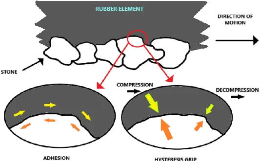
(23) On the other hand, the vertical stresses caused by the loads are widely distributed in the support base of the slab, so that the maximum stress transmitted is only a small fraction of the maximum contact pressure. Slip resistance is achieved by using a layer of silica sand and giving the fresh concrete a suitable surface texture, by dragging a burlap and by brushing, grooving, etc. The macrostructure must be rough for high circulation speeds and may be smoother for moderate or low speeds. The type of texture also influences the noise produced in the tread, perceived both inside and outside the vehicles. Hydraulic concrete increases its resistance over time and if the design of the pavement has been correct, its service index decreases more slowly than that of pavements with asphalt layers. [19]. 2.4. Tire-Road Interaction. Statistically there is a significant effect of skid resistance on the wet accident rate. The wet accident rate increases with decreasing skid resistance. Skid resistance is described as the resistance a pavement can offer to a braking car under wet conditions. The main characteristic of a road surface that influences skid resistance is its texture. Wet skid resistance decreases with increasing speed and the levels of skid resistance achieved are governed by the interaction between the various components of texture and the tire tread. [9] Clearly, properties of road surfaces that improve tire/road friction will generally have a positive influence on skid resistance. Properties of tires, however, will influence friction for vehicles using those tires but not skid resistance (apart, from the specialized case of test tires on skid resistance of measurement devices). When wet conditions are presumed adhesive forces between the road surface and the car tire can be neglected, i.e. adhesion would not contribute a considerable share to the amount of friction generated [10]. Under these friction conditions can totally be allocated to hysteretic effects within the rubber generated by the asperities of the road surface intruding into the tire tread. Although there are other components of pavement friction (e.g., tire rubber shear), they are insignificant when compared to the adhesion and hysteresis force components. Thus, friction can be viewed as the sum of the adhesion and hysteresis frictional forces [11], as seen in Equation (1). A schematic representation of the phenomena is also shown in Figure 4. 𝐹 = 𝐹𝐴 + 𝐹𝐻. 9. (1).

(24) Figure 4 - Schematic Plot of Hysteresis and Adhesion. 2.4.1 Factors Affecting Pavement Friction Numerous factors can influence the magnitude of the frictional force generated between the tire and pavement surface, and Table 1 presents the most important. Friction must be viewed as a process instead of an inherent property of the pavement. It is only when all these factors are fully specified that friction takes on a definite value. Table 1 – Factors affecting pavement friction. Modified from [53]. Pavement Surface Characteristics. Vehicle Operating Parameters. -Microtexture -Macrotexture. Slip speed: -Vehicle Speed -Braking action. -Material properties -Megatexture/ unevenness. Driving maneuver: -Turning -Overtaking. -Temperature *Critical factors are shown in bold. Tire properties. Environment. -Tread design and condition. -Temperature. -Inflation pressure. -Water (rainfall, condensation). -Foot print. -Snow and Ice. -Rubber composition. -Contaminants: Salt, sand, dirt, mud, debris. -Load -Temperature. -Wind.

(25) The surface must provide enough macro-texture to assist effective drainage of water from the road/tire interface and increase the zone of potential dry contact at the rear of the tire/road contact patch. However, drainage alone is not enough to provide good skid resistance; the water film can only be broken if the road surface has a good micro-texture on which localized high pressures are built up [12]. Some researchers have indicated that micro-texture is the single most important factor at both low and high speeds in providing adequate friction at the tire pavement interface [13]. Otherwise, the PIARC experiment strongly confirmed that macro-texture is recognized as a major contributor to friction safety characteristics for several reasons. The most well-known reason is the hydraulic drainage capability that macro-texture has for wet pavements during or immediately after a rainfall. This capability will also minimize the risk for hydroplaning. Another reason is that the wear or polishing of macro-texture can be interpreted as it changes its value over time for a section of road [11].. 2.4.2 Pavement Surface Characteristics To analyze the effects that the pavements (flexible and rigid) cause in vehicles, it is necessary to use small scales that allow to appreciate magnitudes of the order of tenths of a millimeter or even smaller. The A.I.P.C.P. proposed a classification of surface geometrical characteristics based on wavelengths and amplitudes of irregularities, as shown in Table 2. Table 2 - Classification of surface irregularities of a pavement (flexible or rigid). RANGE OF DIMENSIONS (APROX.) HORIZONTAL VERTICAL 0 - 0.5 mm 0 - 0.2 mm 0.5 - 50 mm 0.2 - 10 mm 50 - 500 mm 1 - 50 mm 0.5 - 5 m 1 - 20 mm 5 - 15 m 5 - 50 mm 15- 50 m 10 - 200 mm. NAME *MICROTEXTURE *MACROTEXTURE *MEGATEXTURE *SUPERFICIAL REGULARITY. Short waves Medium waves Long waves. The vehicle-road interaction causes these surface irregularities to influence to a greater or lesser degree, depending on their wavelength. Figure 5 shows the range of irregularities of flexible and rigid pavements that affect the user; however, some of them are necessary for the safety of vehicles. [19]. 11.

(26) Figure 5 - Influence of the range of surface irregularities in the phenomena of interaction between vehicles and the road. [12].

(27) Chapter 3 System Design 3.1 Mechanical characterization of pavement surface 3.1.1 Differentiation of equipment The following diagram in Figure 6 shows a schematic representation of some of the equipment used nowadays for pavements surface measurement and characterization divided by application and mobility.. Figure 6 – Example of equipment used to characterize asphalt. For our experimentation we had access to the British pendulum and the sand patch test.. 3.1.2 British Pendulum Test (Microtexture) Description The purpose of the procedure is to obtain a Slip Resistance Coefficient (S.R.C.) which, maintaining a correlation with the physical coefficient of friction, evaluates the anti-slip characteristics of a pavement surface. The results obtained by this test are not necessarily 13.

(28) proportional or correlative with friction measurements made with other equipment or procedures. This test, as seen in Figure 7, consists in the loss of energy measurement through a pendulum of known characteristics provided at its end of rubber. The edge rubs with a certain pressure on the surface to be tested and on a fixed length. This energy loss is measured by the supplementary angle of the pendulum oscillation. The test method can also be used for measurements on industrial buildings pavements, laboratory tests on specimens, tiles or any type of sample of finished flat surfaces. [15] For further information about the experimental procedure to prepare the equipment, please refer to Appendix A.. Figure 7 - British friction pendulum (ASTM E 274). Calculation Although the British pendulum tester is not a new device, further discussion to review certain important aspects of the tester performance would be beneficial. The basic concepts of design and operation of the British pendulum tester were described by Giles et al. and by Kummer and Moore [16]. Figure 8 shows a schematic of the tester. The differential equation of motion derived from the energy conservation is the following mathematical expression: 𝐼𝜃̈ + 𝑊𝐿𝑠𝑖𝑛𝜃 = 𝐹𝐿(𝑠𝑖𝑛𝜃 + 𝜇𝑐𝑜𝑠𝜃) Where:. (2).

(29) 𝜃 = angular displacement of the pendulum arm from vertical position, 𝐼 = moment of inertia at the center of rotation, 𝑊= weight of the arm, 𝐿 = distance from the center of rotation to the slider, 𝐹 = normal force applied by the rubber slider to the test surface, and 𝜇 = coefficient of friction of the test surface.. Figure 8 – Schematic of British Pendulum tester. The variable that is most important for the performance of the British pendulum tester is the normal force, F, applied by the rubber slider as it is propelled over the teste surface. The sensitivity of the British pendulum tester to the slider normal force can be calculates as: 𝑆𝐹𝑁 =. ∆𝐵𝑃𝑁 ∆𝐹𝑁. = 1.83. 𝐵𝑃𝑁 𝑁. (3). The slide resistance coefficient of the British pendulum is obtained as following: 𝑆. 𝑅. 𝐶. =. 𝐸𝑓𝑓𝑒𝑐𝑡𝑖𝑣𝑒 𝑟𝑒𝑎𝑑𝑖𝑛𝑔 (𝐹𝑅𝑠) 100. (4). The measurements made on the pavement are always affected by the temperature variations of the rubber and the surface tested; therefore, to the value obtained from the pendulum is added a factor to the effective reading. Further information about the temperature correlation factor can be found in Appendix A. For road quality purposes, the Mexican government suggested Table 3 for friction values measured with the British pendulum in wet pavement (critical condition):. 15.

(30) Table 3 - Microtexture values proposed by the Mexican government. [17]. 3.1.3 Sand Patch Test (Macrotexture) Description This test method is suitable for field tests which determines the average thickness of the macrotexture of the surface of the pavement. The knowledge of the thickness of the macrotexture serves as a tool in the characterization of the surface textures of pavements. When used in conjunction with other physical tests, the thickness of the macrotexture derived from this test method can be used to determine the sliding resistance capacity of the materials in pavements or the suggestion of a better finish. When used with other tests, care must be taken that all of them apply to the same place. The measurements of the thickness of the texture produced using this method of the test is influenced by the characteristics of the macrotexture of the surface. The particle shape of the aggregate, size and distribution are characteristics of the surface texture not considered in this procedure. This test method does not attempt to provide a complete qualification of surface texture characteristics. The values of the thickness of the surface macrotexture in the pavement determined by this method, with the material and procedures established here, do not necessarily agree or correlate directly with other surface texture measurement techniques. The surface of the pavement to be sampled using this test method should be dry and free of any construction debris, surface debris, and loose aggregate particles that could be removed or displaced during normal environmental and service conditions. [18]. Experimental Procedure The materials and standard test method consist of a uniform amount of material, a container of known volume, a screen suitable for protection against the wind, brushes to clean the surface, a flat disk to disperse the material on the surface and a ruler or any other device to determine the.

(31) area covered by the material, all of these shown in Figure 9. A weighing scale is also recommended to ensure the consistency of the measurements of each assay. Further information about more test procedure details and its required equipment please refer to Appendix A.. Figure 9 – Sand patch test (ASTM E 965). Calculation Cylinder volume. - Calculate the internal volume of the test cylinder as follows:. V=. 𝜋∗𝜙2 ∗𝐻 4. (5). Where: V = internal volume of the cylinder, in3 (mm3), 𝜙 = diameter of the test cylinder, in (mm), and 𝐻 = cylinder height, in (mm). Average thickness of the macrotexture of the pavement. - Calculate the average of the macrotexture of the surface using the following equation:. H=. 4∗𝑉 𝜋∗𝜙2. Where: H = average thickness of the macrotexture of the surface, in (mm), 𝑉 = volume of the sample, in3 (mm3), and 𝜙 = average diameter of the area covered by the material in, (mm).. 17. (6).

(32) For road quality purposes, the Mexican government suggested Table 4 for macrotexture values measured with the Sand patch test in dry pavement: Table 4 - Macrotexture values proposed by the Mexican government. [17]. 3.1.4 International Friction Index Description This section presents a description to obtain the International Friction Index (IFI) from texture and slip resistance measurements, and finally, its interpretation and application to evaluate the surface conditions of the pavement, in the interest of road safety. The sliding resistance capacity was evaluated in two different ways: •. Directly measuring the coefficient of friction between the tire and the wet pavement. •. Analyzing the macrotexture or the surface drainage capacity of the pavement (to estimate the reduction in adherence that occurs when increasing speed).. The procedure is presented to determinate the IFI using the British Tester and the Sand Patch Test in road sections with several surface conditions. An example to calculate the values of the IFI is presented step by step. Showing tables of field data and later the processing of said data, until reaching the IFI value characteristic of the section. The PIARC model can be used in the administration of pavements establishing levels of intervention of the IFI, considering certain values or minimum levels of friction and texture, according to the prevailing conditions and the needs required in each type of road. To do this, a diagram was created to indicate the relationship between the friction values, FRs, and the texture values, TX, as shown later on this document. In conclusion, the main advantage is the obtainment of a common scale of friction values called IFI in which all the results of friction measurements in road pavements and airports are.

(33) included with an acceptable precision. Final discussions are made about its interpretation and implementation to generate a relationship between the results measured and our acoustical system. [52].. Calculation The PIARC model is the basis of the definition of the International Friction Index, IFI, through the parameters F60 and Sp. Thus, the IFI of a pavement is expressed by the pair of values (F60, Sp) expressed in parentheses and separated by a comma; the first value represents the friction and the second the macrotexture. The first is a dimensionless number and the second is a positive number with no limits and with units of speed (km/h). The friction zero value indicates perfect slip and the value one, grip. It is not possible, for the moment, to describe with a simple relation the second number that makes up the IFI. During the elaboration of the model, and from the data of the PIARC experiment, it has been verified that the velocity constant Sp can be determined by means of a linear regression in function of the field measurement of the macrotexture (TX) such that: Sp = a + (b ∗ TX). (7). Where the values of the constants “a” and “b” for the Sand Patch Test equipment (ASTM E965) are: a = −11.6 , b = 113.6 The value of the FR60 constant is determined using the friction value FRs obtained in the field with some equipment at the slip speed S, where we obtain: FR60 = FRs ∗ 𝑒. 𝑠−60 𝑆𝑝. (8). Finally, the desired value of F60 is obtained through the following correlation with FR60 established by the PIARC experiment: F60 = A + (B ∗ FR60). (9). Where A and B are constants according to the equipment used to measure Friction, and their values for the British Pendulum Tester are: s = 10 km/hr, A = 0.056, B = 0.008. 19.

(34) The knowledge of these parameters also allows knowing the estimated reference curve of friction as a function of the sliding speed according to the following equation: F(s) = F60 ∗ 𝑒. 60−𝑠 𝑆𝑝. (10). The representative Sp and F60 values are replaced for each section given. Once these parameters have been calculated, and using Equation (10), the estimated friction values F for the velocity of time are calculated.. Acceptance/Rejection Graph The PIARC model can be used in the administration of pavements establishing levels of intervention of the IFI, considering certain values or minimum levels of friction and texture, according to the prevailing conditions and the needs required in each type of road. To do this, a diagram is used that relates the texture values (TX) with the friction values (FRs) in the axes, and this applies to any equipment used to measure these parameters. In the diagram is located the curve that will define the border of minimum permissible values, friction (F curve) and the T Line related to the recommended minimum value of texture. [20]. Figure 10 shows how each area of the graph should be interpreted, and thus be able to consider whether the section under study has the proper characteristics of friction and texture. This graph can be used for two purposes: •. The first case as support to know what kind of texture will give us the speed of operation, such that for critical conditions (wet pavement), the vehicles operate safely.. •. The second, as a road adviser, establishing whether to improve the micro- or macrotexture..

(35) Figure 10 - Interpretation areas of the diagram Friction vs. Macrotexture [15]. The interpretation of each of the quadrants in Figure 10 is as follows: I.. II.. III.. IV.. 3.2. In the first quadrant we find that the pavement surface requires improving the macro texture, this may be possible by improving with the placement of a seal irrigation or a micro folder with the appropriate design that allows to dislodge the volume of water that is present by the specific precipitation from that place. In the second quadrant, (following clockwise) according to our limits of F60 and Sp, we will find the points that fulfill with an adequate micro- and macro texture for the needs of our road. In the third quadrant, we found that it is necessary to improve the micro texture, that this could be if the quality of the stone material of the folder is improved (or if hydraulic concrete is used, taking care that it has a good scratch). In the fourth quadrant, the most critical situation of the pavement is presented, since it is necessary to improve both, micro- and macro texture.. Acoustic parameters of road surface. 3.2.1 Modeling of random ground roughness effect by an effective impedance Natural grounds can exhibit small scale geometric irregularities, compared to the acoustic 21.

(36) wavelength, known as ground roughness. Ground roughness has noticeable effects on outdoor sound propagation, since it shifts the ground dip due to the ground effect towards the lower frequencies and it leads to the formation of a surface wave. In the context of prediction methods improvement for outdoor sound propagation, using an effective impedance appears to be a useful approach to model the effects of surface roughness. The boss model approach allows to express an effective impedance Zeff (or an effective admittance βeff= 1/Zeff) for a ground roughness formed by regular scatterers, such as semicylinders [36], as shown in Figure 11.. Figure 11 - Wave vector K0 incident to a surface containing cylinders of radius a and mean center-tocenter spacing b [37].. The effects of roughness are considered as a correction to the surface admittance βS, and Zeff is given by: 1 𝑍𝑒𝑓𝑓. = βeff = βs + βR. (11). 1. Where βs is surface admittance (𝑍𝑠), Zs is base impedance, and the correction βR is function of the angles θi and φ, the frequency, and other parameters depending of the scatterers’ size, shape and spacing. An effective impedance model for random roughness was developed in [36]. Using the Small Perturbation Method (SPM), it models the mean effects of random ground roughness characterized by a roughness spectrum, such as the Gaussian roughness spectrum which is defined by two statistical parameters. Just like the boss model formulation, for an absorbing ground, the ground roughness effect is modeled as a correction to the base admittance of the ground surface. In the SPM model for random roughness a 2D rough surface showing a small and slowlyvarying roughness is considered, as shown in Figure 12. In this figure K0 and its modulus are.

(37) respectively the wave vector and the wave number in the air, with C0 the sound speed in the air, ξ(x) is the height profile, θi is the angle of incidence, Z0 is the characteristic impedance of the air and Zs is the impedance of the surface.. Figure 12 - Wave vector K0 incident to a rough surface ξ. Two dimensional TLM simulations of 50m propagation above absorbing and rigid random rough grounds (whose roughness was defined by a Gaussian spectrum) were performed in [36], and the results were compared to analytical solutions calculated with the SPM effective impedance model, which showed that the SPM effective impedance accurately takes into account the mean effects of roughness on sound level spectra, and also correctly models the roughness induced surface wave. SPM effective impedances were implemented in FDTD and TLM codes by approximating the effective impedance by a sum of rational functions, using the vector fitting technique to identify the coefficients of these functions. FDTD and TLM numerical methods with SPM effective impedance have been proven to be efficient and useful for simulating complex middle-range propagation cases with time-domain methods, as they allow to consider quite easily the mean effects of a statistically defined roughness. [36] It should be pointed out that in order to be used in time domain, an impedance model must be physically admissible and verify reality, causality and passivity conditions [38,39]. The Miki model with thickness effect was the base impedance model considered to derive the SPM effective impedance for the considered grounds using (47). Recent studies [40,41] showed that the Miki model is actually not physically admissible, and not the best suited model for longrange outdoor sound propagation predictions despite its common use. Furthermore, this SPM effective impedance approach should still prove functional using more refined base impedance models, such as the slit pore model [42]. A promising application for effective impedance models and particularly for the SPM model would be to use them in engineering methods for an acoustic characterization of road pavements. This would require experimental data to characterize roughness spectra of pavements.. 23.

(38) 3.2.2 Theoretical model of acoustic system proposal An outline of this configuration is presented in Figure 13, which is considered a primary point source situated at a height Zs and a receiver located at a height Zr above the ground surface. This porous surface is treatment as a flat surface, consisting of a semi-infinite field, an absorbing layer on a rigid layer or a combination of different absorbent layers. In all cases, the surface is homogeneous, and the propagation is in the atmosphere.. Figure 13 - Geometry to study the attenuation between source and receiver in presence of a porous ground formed with several absorbent layers. The sound pressure at the receiver is the sum of the direct signal, which comes from the real source, plus the reflected signal from the ground, which is assumed to come from the image source. The method consists on measuring the sound level difference from two microphones close to the surface and calculating the level difference according to an impedance model of the ground. To solve this problem, it is assumed that the total potential is because a direct contribution from the source to the receiver, and a contribution of the reflected part in porous surface, of the form [31]. 𝜙=. 𝑒 𝑖𝑘𝑅1 4𝜋𝑅1. + 𝑄1. 𝑒 𝑖𝑘2𝑅2 4𝜋𝑅2. ,. (12). where Q1 is the reflection coefficient of the spherical wave for the point source on the outer surface with a finite impedance, R1 is the distance between the point source and the receiver and R2 is the traveled path by the reflected wave between source and receiver, as shown in Figure 13. Knowing the angle of incidence of the reflected wave and the specific admittance β, which defines the properties of the absorbing surface, the reflection coefficient of the spherical wave can be calculated with the expression: 𝑄1 = 𝑅𝑝 + (1 − 𝑅𝑝 )𝐹(𝑤1 ). (13).

(39) where: 𝑐𝑜𝑠𝜃−𝛽. 𝑅𝑝 = 𝑐𝑜𝑠𝜃+𝛽. (14). is the reflection coefficient of the plane wave, and the function F(w1) is called the boundary loss factor, given by the expression: 2. 𝐹(𝑤1 ) = 1 + 𝑖 √𝜋𝑤1 𝑒 −𝑤1 𝑒𝑟𝑓𝑐(−𝑖𝑤1 ). (15). where erfc () is the complementary error function, and w1 is the numerical distance that is calculated as: 1. 𝑤1 = √2 𝑖𝑘𝑅2 (𝑐𝑜𝑠𝜃 + 𝛽). (16). To use these equations, a model for the specific impedance of the absorbing surface was needed. Preliminary, in this work three different situations have been considered. The simplest case is a semi-infinite homogeneous medium that fills the bottom space bounded by the surface. Then, the specific admittance has the expression: 𝛽 = 𝑚1 √𝑛12 − 𝑠𝑖𝑛2 𝜃. (17). were: 𝑛1 =. 𝑘1 𝑘. ,. and. 𝜌. 𝑚1 = 𝜌. 1. (18-19). In Equations (18-19) k1 is the complex wave number of propagations in porous medium and ρ1 the density of the porous medium. If the absorbing surface is comprised of a layer of porous material above a rigid surface, the admittance specific expression is: 𝛽 = −𝑗𝑚1 √𝑛12 − 𝑠𝑖𝑛2 𝜃tan (𝑘𝑑1 √𝑛12 − 𝑠𝑖𝑛2 𝜃). (20). where d is the thickness of the porous layer in contact with the surface. Finally, if we consider two porous layers, the specific admittance is given by:. 𝛽=. −𝑗𝑚1 √𝑛12. −. 𝑠𝑖𝑛2 𝜃. tan(𝑘𝑑1 √𝑛12 −𝑠𝑖𝑛2 𝜃)+𝑔1 tan(𝑘𝑑2 √𝑛22 −𝑠𝑖𝑛2 𝜃) 1+𝑔1 tan(𝑘𝑑1 √𝑛12 −𝑠𝑖𝑛2 𝜃)tan(𝑘𝑑2 √𝑛22 −𝑠𝑖𝑛2 𝜃). where: 25. (21).

(40) 𝑔1 =. 𝑚2 √𝑛22 −𝑠𝑖𝑛2 𝜃 𝑚1 √𝑛12 −𝑠𝑖𝑛2 𝜃. (22). This dimensionless factor characterizes the change of acoustic propagation properties between the two-porous media. [32,33] According to this model, the ground attenuation will be: 𝑅. ∆𝐿 = 20 𝑙𝑜𝑔10 [|1 + 𝑄 𝑅1 𝑒 𝑗𝑘0 (𝑅2 −𝑅1 ) |] 2. (23). Thus, a ground impedance model is required to calculate the effect of this boundary in the sound field. Impedance models of one, two, three or four parameters can characterize each of the ground layers. Let us consider a plane wave incident on a surface with angle 𝜃0, characterized by acoustic impedance Zs and propagation constant ks, as seen in Figure 14.. Figure 14 - A plane wave incident on a homogeneous medium.. The impedance model, Zs, is established for the ground. In this case, a homogeneous locally reacting ground is assumed with normalized acoustic impedance given by the Delany-Bazley equation for one parameter model [34] 𝑧𝑠 = (1 + 0.0571𝐸 −0.754 + 𝑗0.087𝐸 −0.732 ). (24). where E=r0f/σ, r0 is the air density, σ is the flow resistivity, and f the frequency. This model, which depends on just one parameter (the flow resistivity) has been adopted in some works for calculating the excess attenuation of grounds [35]..

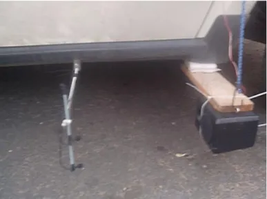
(41) 3.2.3 Experimental methodology based on previous work The experimental measurements were performed along several pavements, in Mexico City. The following equipment was used: two small acoustic sensors, with frequency response of 20–20,000 Hz; small directional source with frequency response of full range; audio interface of two channels, with sampling frequency of 96 kHz; a laptop and software for signal processing. The two sensors were mounted on a support and a base of wood for the source and were installed in a sports utility vehicle as shown in Figure 15. The sensors were placed at different heights from the soil: 0.06 m and 0.165 m; the source was at a height of 0.165 m, and the distance between sensors and source was 0.45 m. The geometry setup recommended by ANSI S1 standard [43] was slightly modify due to the conditions and the portability. The purpose of this setup was to measure the sound level difference of two sensors, when the source radiates a MLS (Maximum Length Sequence) signal from a horizontal distance to the sensors. The parameters of a ground impedance model were modified and compared with the experimental curve. The difference in the impedance of the soil between the experimental and the theoretical curves is minimized [44]. The ANSI S1.18 standard covers a frequency range of 250 Hz to 4 kHz. It recommends using a signal with level at least 10 dB above the background noise level. In any case, a cover was used for the sensors. The soil must be flat. The recommendations of the standard were accomplished.. Figure 15 - Experimental setup.. The source can be seen oriented in the direction of the support holding the two sensors. Firstly, a measurement was made in a static position, then at different speeds 10-100 km/h for different pavements along of the city [24]. Figure 16 shows the level difference curves measured at various speeds: 0, 20, 50 and 100 km/h. It shows that, as the speed increases, the resulting curve is not affected by aerodynamic and background noises due to the unwanted reflections and the noise was filtered. 27.

(42) 50 40. 100 km/h. 50 km/h. 20 km/h. 0 km/h. 30. L. exp. (dB). 20 10 0 -10 -20 -30 -40. 500. 1000. 1500. 2000 2500 Frequency (Hz). 3000. 3500. 4000. Figure 16- Experimental difference curves at different speeds with noise filtered.. Getting surface parameters Weather conditions are important, since the determination of sound propagation requires information on temperature, relative humidity and barometric pressure as a function of height near the propagation path. These values determine the sound speed profile. Ideally, the altitude at which the meteorological data are collected should reflect on the application. In order to make the comparison and adjustment between the experimental and theoretical curves, an algorithm in Matlab was implemented establishing all the ranges for each parameter under test, and a nonlinear programming that attempts to find a constrained minimum of a scalar function of several variables starting at an initial estimate. This is generally referred to as constrained nonlinear optimization [45]. For more information about the Matlab Graphical User Interface (GUI), go to Appendix B. The frequency fitting range for comparing the theoretical curves, for this case is 1 – 5.5 kHz, due to the absorption and reflection in the path. In Figure 17, the result shows the three parameters and two related parameters (texture and µ), in the case of a speed of 100 km/h: σ = 0.78 x 106 N s/m4, φ = 0.68 and ζ = 0.46; the graphic shows the experimental signal (red) and the theoretical (black) curve, displaying minor discrepancies between them..

(43) 25 4.  = 0.789 e006 N s/m. 20.  =0.68. Sp=0.46. Level Difference (dB). 15 10 5 0 -5 -10 -15. Experimental Theoretical. -20 -25. 500. 1000. 1500. 2000. 2500 3000 3500 Frequency (Hz). 4000. 4500. 5000. 5500. Figure 17- Theoretical and experimental level difference curves for the asphalt at 100 km/h.. Table 5 displays the three parameters obtained at different speeds, acquired along 100 km of some streets and avenues. As can be seen, the three parameters are consistent and reasonable, with the flow resistivity parameter showing more variation, between 0.6 - 1.2 x 106 N s/m4. According with these results, the texture of the pavements can be classified in micro and macro textures likewise the friction coefficient was related and estimated [46]. Table 5 - Surface parameters obtained at different speeds.. Figure 18 shows a comparison between factors at 0 and 100 km/h, from which we conclude that for flow resistivity, porosity and shape factor the value is relatively maintained.. 29.

(44) 1 0.9 0.8 0.7 0.6 0.5 0.4 0.3 0.2 0.1 0 Flow resistivity (N s/m^4*10^6). Porosity. 0 km/h. Shape Factor. 100 km/h. Figure 18 - Comparison chart of flow resistivity, porosity and shape factor at 0 and 100 km/h.

(45) Chapter 4 Methods The main experimental methodology was divided in two parts. The first part consisted in measuring the microtexture (friction) and macrotexture of pavement at 5 different street locations around the ITESM – Campus Monterrey, as seen in Figure 19. Meanwhile, the second part consisted in obtaining the acoustic properties from the same asphalt locations in static and dynamic mode. The British pendulum test was used to measure friction, the sand patch test to measure texture, and an acoustic system was proposed to obtain characteristic properties such as porosity, tortuosity, shape factor and flow resistivity of the pavement. The purpose of this experimentation was to compare results between the different methods and create relationships between the mechanical and acoustical pavement characterization systems.. Figure 19– Location of measurements around the ITESM – Campus Monterrey. 4.1 Measurements with Mechanical Equipment 4.1.1 Friction measurement with British Pendulum Test 31.

(46) Figure 20 shows an example of a measurement carried out with the British pendulum at Location 1. Furthermore, Table 6 shows the friction values obtained for each of the five points where the measurements were made at a temperature of 14°C.. Figure 20 – Friction measurement at 1st location. Table 6 – Friction values measured with the British pendulum on road surfaces. According to the values measured it is concluded that the order of friction (S.R.C.) from better to worse is as following: 1) 2) 3) 4) 5). 2nd location (0.633) 1st location (0.564) 3th location (0.531) 4th location (0.521) 5th location (0.507). 4.1.2 Macrotexture measurement with Sand Patch Test Figure 21 shows an example of the measurements carried out with the Sand patch test at Location 3. Furthermore, Table 7 displays the macrotexture values obtained for each of the points where the measurements were made..

(47) Figure 21– Macrotexture measurement at 3th location. Table 7 – Sand patch test measurements (mm). According to the values measured, it is concluded that the order of macrotexture (mm) from better to worse for the five locations is as follows: 1) 2) 3) 4) 5). 5th Location (1.060) 1st Location (0.942) 2nd Location (0.911) 3th Location (0.435) 4th Location (0.203). 4.1.3 International Friction Index The PIARC model is the basis of the definition of the International Friction Index, IFI, through the parameters F60 and Sp. Thus, the IFI of a pavement is expressed by the pair of values (F60, Sp) expressed in parentheses and separated by a comma; the first value represents the friction 33.

(48) and the second the macrotexture. The first is a dimensionless number and the second is a positive number with no limits and with units of speed (km/h). The friction zero value indicates perfect slip and the value one, grip. For the moment it is not possible to describe with a simple relation the second number that makes up the IFI. [52] During the elaboration of the model, and from the data of the PIARC experiment, it has been verified that the velocity constant Sp can be determined by means of a linear regression in function of the field measurement of the macrotexture (TX). The representative Sp and F60 values obtained using Equations (7) to (9) are replaced for each section given. Once these parameters have been calculated, and using (10), the estimated friction values F for the velocity of time are calculated. These values are presented in Table 8, and the behavior curves of the pavement surface are plotted as shown in Figure 22. Table 8 – Calculation of IFI. 1.0 0.9. Friction, F(s). 0.8 0.7 0.6 0.5 0.4 0.3 0.2 0.1 0.0 0. 20. 40. 60. 80. 100. 120. Skidding velocity, s(km/hr) 1° IFI(.323,95.47). 2° IFI(.349,91.93). 4° IFI(.061,11.49). 5° IFI(.312,108.9). 3° IFI(.169,37.86). Figure 22 - Comparison of sections with IFI (F60, Sp). In this graph it can be observed that at a higher speed the friction is decreasing, this is due to the reduction of the contact area between the pneumatic-pavement interface..