Activation Work Analysis Methodology for Body Powered Devices

Texto completo

(1)Instituto Tecnológico y de Estudios Superiores de Monterrey Campus Monterrey School of Engineering and Sciences. Master of Science in Manufacturing Systems. Activation Work Analysis Methodology for Body-Powered Devices. Presented by David Arturo Rodríguez Sánchez Advised by Jorge Armando Cortés Ramírez, Dr.Eng.. Monterrey, Nuevo León, December 1st, 2019..

(2)

(3) Acknowledgments. Acknowledgments To Tecnológico de Monterrey for allowing me to grow in science and as an integral human being. To all the professors that allowed me to grow in knowledge and discipline. As well as the support and patience of my advisor during the development of my research.. To CONACyT for supporting my pursuit of knowledge with challenging research fields, encouraging me to look for novel developments and providing the resources to fulfill my degree.. I thank my family. Especially my mother and two of my siblings, Luis Fernando and Angélica, as they encouraged me to do keep going until the end. To my deceased father from whom I inherited my taste for engineering.. I.

(4) II.

(5) Content. CONTENT ABSTRACT ..................................................................................................................................................... V 1.. 2.. 3.. 4.. INTRODUCTION ......................................................................................................................................... 1. 1.1. BACKGROUND .................................................................................................................................... 1. 1.2. LITERATURE REVIEW ............................................................................................................................ 1. 1.3. USER PERCEPTION ............................................................................................................................... 5. 1.4. JUSTIFICATION.................................................................................................................................... 6. 1.5. HYPOTHESIS ...................................................................................................................................... 6. 1.6. OBJECTIVE ......................................................................................................................................... 6. 1.7. METHODOLOGY ................................................................................................................................. 6. EXPERIMENTAL ANALYSIS ...................................................................................................................... 9. 2.1. CHARACTERIZATION METHOD ............................................................................................................... 9. 2.1.1. STATIC EQUILIBRIUM FREE BODY DIAGRAM ............................................................................................ 10. 2.1.2. STATIC EQUILIBRIUM EQUATIONS ......................................................................................................... 11. 2.1.3. MOMENT OF FORCE........................................................................................................................... 11. 2.1.4. ESTABLISHMENT OF INITIAL CONDITIONS ................................................................................................ 12. 2.1.5. STATIC EQUILIBRIUM ANALYSIS ............................................................................................................ 14. 2.1.6. ELASTIC CONSTANT AND DAMPING FACTOR ............................................................................................ 20. 2.1.7. DEVICE COMPONENTS VIRTUAL MODELLING .......................................................................................... 22. 2.1.8. FORCE-DISPLACEMENT NUMERICAL SIMULATION ..................................................................................... 23. 2.1.9. ACTIVATION WORK........................................................................................................................... 25. 2.2. TEST MECHANISM DESIGN .................................................................................................................. 27. 2.3. FORCE DISTRIBUTION AND ACTIVATION WORK ANALYSIS .......................................................................... 31. RESULTS ................................................................................................................................................... 37. 3.1. CHARACTERIZATION METHOD ............................................................................................................. 37. 3.2. FORCE DISTRIBUTION......................................................................................................................... 39. 3.2.1. LEVER’S COMPARISON ........................................................................................................................ 45. 3.2.2. PULLEY AND LEVER COMPARISON ......................................................................................................... 49. DISCUSSION ............................................................................................................................................. 53. 4.1. ACTIVATION WORK........................................................................................................................... 53. 4.2. ACTIVATION FORCE ........................................................................................................................... 54 III.

(6) Content. 4.3. REDUCTION PERCENTAGE .................................................................................................................... 54. 4.4. CABLE EXCURSION DISPLACEMENT ........................................................................................................ 56. 4.5. FORCE DISTRIBUTION......................................................................................................................... 57. 4.6. METHODOLOGY APPLICATIONS ............................................................................................................ 57. 4.7. BODY-POWERED PROSTHETICS AGAINST MODERN TECHNOLOGY................................................................. 59. 5.. CONCLUSION............................................................................................................................................ 61. 6.. REFERENCES ........................................................................................................................................... 63. APPENDIX A ...................................................................................................................................................... 65 APPENDIX B ...................................................................................................................................................... 69 APPENDIX C ...................................................................................................................................................... 73. IV.

(7) Abstract. Activation Work Analysis Methodology for Body-Powered Devices by David Arturo Rodríguez Sánchez. ABSTRACT Body-powered devices have a dominant position in the market since they provide good functionality, control reliability and mechanical proprioception (the sensorial capacity to perceive one’s own limb without looking at it). In addition, they are lighter and their simple design makes them easy to repair. Body-powered mechanisms commonly consist of a cable attached to the prosthetic device from one end and to the user from the other. The cable must be pulled by either arm flexion or shoulder shrug, depending of the location where the cable is attached to the body of the user. There are two categories: Voluntary Opening (VO) and Voluntary Closing (VC). VO devices will remain closed until the user pulls the cable, while VC devices work in the opposite way. VO devices provide constant grappling once the cable is released. The force exerted to pull the cable is known as “Excursion Force”. The majority of adult users prefer VO body-powered hooks to body-powered hands, passive prosthesis and most electric devices. However, VO body-powered prostheses trade-off is their higher excursion force. Over time, users develop fatigue in their shoulders and the harness starts to irritate their skin. The current research develops an analysis methodology of the work done during the opening of the device, should be referred as “Activation Work” in order to acquire information of the distribution of the excursion force and the consequences of reducing it. The analysis is carried out in a VO body-powered device, Hosmer model 5x Hook. Overall work’s development is divided into three stages: “Characterization Method”, “Test Mechanism Design” & “Force Distribution and Activation Work Analysis”. First stage. Device is digitalized upon cable forces and excursion displacements from literature, its dimensions are unaltered to deduce the elastic constant and damping factor of its elastic band, which are used to define simulation parameters. Cable force and excursion required to open the device are calculated through simulation. Device’s activation work is deduced analytically. If analytical results coincide with experiments (literature’s measurements), then the study moves to the second stage. If not, elastic constant and damping factor deductions as well as estimations are repeated until satisfying literature’s experimental results. Second stage. Four mechanisms are tested to validate the reliability of the analysis methodology. First design, a lever perpendicular to the prosthetic limb. Second design, a lever at 60.0° from the limb. Third design comprehends two levers of different lengths, the larger one at 90.0° and the shorter one at 60.0°. Fourth design is a double pulley system with different radii. Each reducer design is modelled and simulated separately. Activation force distribution is calculated for each design. If activation work is reduced, the process moves to the third stage. If not, levers and pulleys are redesigned repeatedly until achieving activation force reduction. Third Stage. Force distribution is analyzed for each case. The virtual device reproduces literature’s excursion forces and activation work with an accuracy of 98%. Results from lever proposals demonstrates that placing a single lever at 60.0° reduces activation force the most with a percentage of 38% at full excursion displacement. Whereas the highest reduction percentage at half excursion displacement is achieved by the lever at 90.0º with a percentage of 50%. It is concluded that the methodology carried out to deduce the elastic constant and damping factor of the device’s elastic band proves to be reliable, as numerical simulation results replicate literature’s experimental measurements. It is concluded that the analysis method carried out to deduce the elastic constant and damping factor is reliable as it allows the numerical simulation to predict excursion forces and displacements with high accuracy. As both are proven when compared against literature’s measurements. Overall, the characterization method, numerical simulations and analytical deductions prove to be reliable tools for replicating literature’s experimental measurements. Allowing them to be used as validation protocols for mechanical systems. It is concluded that calculating activation work provides insight of how excursion force is distributed after a reducer is installed. For instance, the lower excursion force required is given by the single lever at 60° design; however, it reduces the force in exchange of larger excursion displacements.. V.

(8) Abstract. VI.

(9) 1.. Introduction. 1. INTRODUCTION. 1.1. BACKGROUND. Worldwide healthcare primary concern in the actuality is to enable technological advancements to reach the majority of patients as possible.[4] Disability and rehabilitation represent medical areas of interest for the current work. Specifically, the branch of prosthetic devices, where researchers are continuously developing methods and designs capable of emulating natural body parts functionalities.[4] However, innovative solutions, such as myoelectric prostheses, aim to carefully replicate human appearance in exchange of lower hard work resistance.[11] In contrast, body-powered prostheses mechanisms simpler design possess higher functionality and resistance with appearance far from human.[2]. 1.2. LITERATURE REVIEW. As found in literature, the majority of adult patients prefer body-powered devices to bodypowered hands, passive devices and hands, and electric devices and grippers; only being tightly competed by electric hands.[5] Although, the latter one’s advantage is just its aesthetics. The reason of choosing Body-powered devices is that the shape of the hook allows. 1.

(10) 1.. Introduction. it to pick and hold a wider variety of objects, as well as its roughness allows the user to perform harder work than the hands.[5] The core design consists of a cable attached to the prosthetic device (artificial hand, device or gripper) from one end and to the body of the user from the other. The cable is fastened to the patient by either a harness or a medical tape. The users open the device by pulling the cable.[3] Excursion is performed by arm flexion, “Glenohumeral Flexion”, if the cable is fastened to the corresponding scapula of the prosthetic limb, or shoulder shrug, “ Biscapular. Abduction”, if the cable is fastened the opposite scapula. The closing system is elastic band based; therefore, its gripping force depends directly on the number of bands mounted on it.[3] The manipulation principle and both fastening arrangements is shown in Fig. 1.1.. Fig. 1.1. 𝑎) “Glenohumeral Flexion”. Point 𝐴, cable holder. Point 𝐵, cable-body attachment. Point 𝐻, cable-device attachment. 𝑏) “Biscapular Abduction”. Point 𝐴, cable holder. Point 𝐵, cable-body attachment. Point 𝐻, cable-device attachment. 𝑐) Device diagram. Point 𝐴, cable holder. Point 𝐻, cable-device attachment. Diagrams taken from “Powered Limb Prostheses: Their Clinical Significance”.. Body-powered technology is divided into two categories: Voluntary Opening (VO) and Voluntary Closing (VC). VO devices are normally closed systems, which require the user to pull the cable to open them. VC devices, which are normally open systems, work in the opposite way. Therefore, the excursion of the cable open will them. VO prostheses advantage is their automatic grapple once the cable is released.[9] 2.

(11) 1.. Introduction. Body-powered limbs meet adaptability, due to their relatively straightforward mechanisms; as well as availability and acceptability due to their functional design. The current study is working the most commonly wore device, the Hosmer model 5x, which is presented in Fig. 1.2. As it is perceived, the tension of the band establishes the grappling force of the device.. Fig. 1.2. 𝑎) Rightside and 𝑏) frontside of Hosmer prosthetic model 5x Hook. Picture taken during the current work. Complete prosthesis is shown in Fig. 1.3. The artificial limb is known as “socket” and is handcrafted to fit each user specifically. Device and socket are attached to the user by fastening a harness to one of their shoulders. Harness used for the current work is presented in Fig. 1.4.. Fig. 1.3. Hosmer model 5x Hook coupled with a carbon fiber socket and excursion cable attached.. 3.

(12) 1.. Introduction. Fig. 1.4. Body-powered prosthetic system attached to harness. Body-powered prosthetic limbs had its peak development in USA during the early 1950’s. At that time, “Glenohumeral Flexion” and “Biscapular Abduction” were established as their manipulation principle.[2] They provided good functionality; as well as being simple, relatively inexpensive and easy to repair. In addition, they provided mechanical proprioception, that is, the cable in the system allowed the user to know the position of the device without actually looking at it.[9] Disadvantages, the harness may be restrictive and uncomfortable, as well as the gross movements required to activate the device may be undesirable [9]. Body-powered devices major complaint is activation force, which significantly large. This is uncomfortable and can lead to fatigue and irritation of the shoulder and the axilla.[5] In order to properly use a body-powered prosthesis, the device must be mechanically efficient and require a low activation force. As found in literature, nearly all tested VO devices were inefficient and required high activation forces that users might find uncomfortable [8]. Therefore, the study of the performance of VO devices is relevant. For instance, [7] measured the mechanical performance of VO devices for adults. Albeit, there are no recent data available on the mechanical efficiency of VO devices. Then, [7] compares different VO devices for adults by measuring the mechanical work, energy dissipation, maximum cable force and excursion, pinch force, opening span, and device mass. Although, it does not give a concrete insight of the proneness of the devices to fatigue the user. 4.

(13) 1.. 1.3. Introduction. USER PERCEPTION. The current work met two VO body-powered device users who were asked, among other design aspects, about their perception of the excursion force. They are chosen to represent opposite populations in order to reduce the bias of the research. The first user is a male worker in his 40’s who has lost both of his arms. The second user is a female high school student who was born with just one hand. The questionnaire is presented in Table 1.1. Table 1.1. Body-powered devices performance questionnaire. Question. Answer. General comments regarding the prosthesis How difficult is it for you to dress? How difficult is it for you use the toilette? Did you take a course before using the prosthesis? How many hours a day do you use your prosthesis Does using the prosthesis cause fatigue at any moment? The most relevant question for the current research is: “Does using the prosthesis cause fatigue at any moment?” To which the first user, a male worker in his 40’s who has lost both of his arms, answered: “The prosthetic limb is light to carry but requires certain force to operate the hook. It does not generate fatigue in me as I does not carry it during the whole day. Although, the activation system requires a more comfortable closing system, to prevent it from exhausting the user.” The second user, a high school female student answered: “I’ve been practicing with it for months. I use the prosthetic limb most of the day; although, it gets difficult to activate the hook at the end of the day. I require certain amount of force to open the hook and makes me feel tired over time.” From previous answers, excursion force is demonstrated to be a drawback of the VO bodypowered devices. Furthermore, the energy of the user is reduced over time, which increase the difficulty of operating the device. Therefore, taking into account the work required by the system is important to predict the efficiency of the system. 5.

(14) 1.. 1.4. Introduction. JUSTIFICATION. VO body-powered devices major disadvantage is their excursion force, which is the highest among its competitors due to its closing mechanism. For instance, the majority of users have reported irritation in the area of skin are the cable is attached to the user, as well as fatigue in their shoulder used to open the device. In addition, measurements such as in G. Smit and K. Berning furtherly confirm their VO higher excursion forces. However, reducing such forces mechanically causes an increase in cable displacement. Therefore, a analyzing force distribution during activation enables the possibility to find an equilibrium point between force decrease and displacement growth.. 1.5. HYPOTHESIS. Analyzing the activation work of a body-powered device provides information regarding force distribution during the opening forces and how it is affected when a force-reducer is installed.. 1.6. OBJECTIVE. The focus of the work is to develop an analysis methodology of the activation work required to open the device in order to perceive force distribution and its response if a force reducer should be installed. In addition, four excursion force reducers are tested to furtherly validate the performance of the methodology.. 1.7. METHODOLOGY. The current work development is divided into three stages: 1. Characterization Method. A virtual model of the current device is developed and simulated. Static equilibrium analysis is used to determine the tensions generated in the band of the device. Data of forces and displacements are taken from experiments and 6.

(15) 1.. Introduction. applied as initial conditions. Tensions deduced from the static analysis are plotted and linearly approximated. The band is substituted by a spring during the numerical simulations and the linear equation is used to determine its simulation parameters. Results of forces and displacements are plotted and integrated in order to deduce the activation work done, if values are congruent with literature’s experimental measurements, then the analysis is proven to be reliable and the work proceeds to the next stage. If values do not match literature’s data, the analysis is reviewed and re-done until satisfying the required values. 2. Test Mechanism Design. Four designs are proposed to further prove the reliability of the analysis methodology, and to reduce excursion force. First design is compound by a lever with a length of 75 mm located at 90° from the prosthetic limb and a lever with a length of 50 mm at 60°; the shorter lever is attached to the device, while the larger lever is actioned by the user. Second design is just one lever with a length of 75 mm located at 90° from the prosthetic limb, a hole at 43.3 mm from the bottom functions as an attachment; the lever is attached to the device from the hole, while its upper side is pulled by the user. Third design is a lever of the same length but located at 60° from the prosthetic limb, a hole at 50 mm from the bottom serves as the attachment; once again, the lever is attached to the device from the hole, while the user pulls the upper side. Fourth design consists of a pulley with a radius of 43.3 mm mounted over another pulley with a radius of 75 mm; the smaller pulley is attached to the device, while the larger one is actioned by the user. The four designs are modelled and simulated in solid works. If excursion forces are reduced, the work 3. Force Distribution and Activation Work Analysis. Force reduction is compared to displacement increase in each test mechanism and activation work is calculated, then force distributions are compared. Development stages are arranged in the flowchart shown in Fig.1.5.. 7.

(16) 1.. Introduction. Fig. 1.5. Flowchart of validation process for definitive proposal selection. This analysis methodology serves as a validation tool for any given body-powered device. As a demonstration, it is applied in the current work to analyze work distribution when peak activation force is reduced.. 8.

(17) 2.. Experimental Analysis. 2. EXPERIMENTAL ANALYSIS. 2.1. CHARACTERIZATION METHOD. Current research is working upon "Efficiency of voluntary opening hand and hook prosthetic devices: 24 years of development?"[17] experimental measurements of cable forces, excursion displacements and activation work of the Hosmer model 5x hook. In order to design the activation work reducer, the current work is transitioning the physical device to a virtual counterpart, maintaining critical dimensions while discarding aesthetics. To accurately reproduce the behavior of the device, four different positions are considered and mathematically analyzed through static equilibrium analysis. Each position corresponds to a specific cable excursion displacement, from which a determined force is generated. Displacement and forces are taken from [18] as initial conditions for the analysis. The objective of the analysis is to determine the tensions generated in the elastic band. Tensions are then used to plot the behavior of the force during the activation of the device. The resulting pattern is approximated by a linear function from which equation describe the elastic constant and damping factor of the band. Both elastic constant and damping factor are used as numerical simulation parameters. The accuracy of the parameters is proven by replicating the results of [19] through SolidWORKS Motion Analyzer. Simulated cable forces are plotted and their behavior compared to literature’s experimental measurements. The plot is 9.

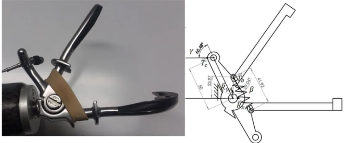
(18) 2.. Experimental Analysis. approximated by a second order function and its equation is integrated in order to deduce de activation work of the device. Activation work is compared to [20] results. Accuracy of the analysis is proven by comparing simulated forces and activation work against literature’s measurements. Once reliability of the numerical simulation is demonstrated, the method is used to test activation work reducers.. 2.1.1 STATIC EQUILIBRIUM FREE BODY DIAGRAM Free body diagrams are required to solve the static equilibrium analyses.[10] Values of distances and angles are taken from the original model, just aesthetic details are excluded. The original system is shown in Fig. 2.1. Two positions are presented as a picture and as its respective diagram: closed and fully opened.. Fig. 2.1. 𝑎) Device in its initial position. 𝑏) Initial position diagram, length of the lever 50 mm, length of the hook 120 mm, length of the elastic band 26.43 mm, distances from the middle point in the grappling area to the rotation axis 115 mm and angle of the lever 60°. 𝑐) Device in its full aperture position. 𝑑) Final position diagram, device’s aperture 60° and length of the elastic band 42.89 mm.. 10.

(19) 2.. Experimental Analysis. As a mathematical tool, the elastic band is substituted by a spring in the diagram. The vector of the force exerted by the cable is located in the geometric center of the band.. 2.1.2 STATIC EQUILIBRIUM EQUATIONS The static analysis is carried out by solving the equilibrium Eqs. (2.1), (2.2) and (2.3).. ∑ 𝐹⃑𝑥 = 𝐹⃑𝑥1 + 𝐹⃑𝑥2 + 𝐹⃑𝑥3 … + 𝐹⃑𝑥𝑛 = 0. (2.1). ∑ 𝐹⃑𝑦 = 𝐹⃑𝑦1 + 𝐹⃑𝑦2 + 𝐹⃑𝑦3 … + 𝐹⃑𝑦𝑛 = 0. (2.2). ⃑⃑⃑𝐴 = 𝑀 ⃑⃑⃑1 + 𝑀 ⃑⃑⃑2 + 𝑀 ⃑⃑⃑3 … + 𝑀 ⃑⃑⃑𝑛 = 0 ∑𝑀. (2.3). Where ∑ 𝐹⃑𝑥 stands for “Sum of Forces” upon the 𝑥-axis, ∑ 𝐹⃑𝑦 the “Sum of Forces” upon the 𝑦⃑⃑⃑𝐴 the “Sum of Moments of Force” upon any point. Since the system is in axis and ∑ 𝑀 equilibrium, all of the sums must be equal to zero.[10]. 2.1.3 MOMENT OF FORCE A “Moment of Force” also known just as “Moment”, is the cross product of the force applied to an object and the distance from a fixed point within it. Specifically, the force component that causes is perpendicular to the aforementioned distance. Such distance is known as “radius to the rotation axis”.[10] Moment are deduced by implementing Eq. (2.4).. ⃑⃑⃑ = 𝑟⃗ × 𝐹⃗ = |𝑟⃗| ∙ |𝐹⃗ | sin(𝜃) 𝑀. (2.4). 11.

(20) 2.. Experimental Analysis. Where 𝑟⃗ stands for radius from the rotation axis to the applied force, 𝐹⃗ represents the total magnitude of the applied force and |𝐹⃗ | sin( 𝜃) its perpendicular component relatively to the radius of rotational radius. Diagram in Fig. 2.2 shows a force applied to an object, its components and the moment produced by it.. Fig. 2.2. Diagram of moment produced in a body. ⃑⃑⃑⃗ 𝐹𝑦 = 𝐹⃗ sin⁡(𝜃) is the force component ⃑⃑⃑⃗𝑥 = 𝐹⃗ cos⁡(𝜃) the parallel component. perpendicular to the rotational radius and 𝐹 Once equations are stablished, next step is to generate diagrams of the device.. 2.1.4 ESTABLISHMENT OF INITIAL CONDITIONS Literature’s experimental cable force and displacement graph are reproduced in Excel due to blurriness in their original form. Resulting graph is shown in Fig. 2.3.. Cable Excursion Force. Cable Release Force. 30.0. Cable Force (N). 24.0 18.0 12.0 6.0 0.0 0.0. 10.0. 20.0. 30.0. 40.0. Cable Displacement (mm). Fig. 2.3. Data is taken from Force-Displacement graph found in "Efficiency of voluntary opening hand and hook prosthetic devices: 24 years of development?". 12.

(21) 2.. Experimental Analysis. As seen in Fig. 2.3, cable forces present a delay during first millimeters, and then they have a drastic increase, followed by an almost imperceptible growth and another drastic increase at the end. It is worth noting, though, that literature’s device is fully opened at around 46 mm of cable excursion, which suggested that the second increase is caused by the own mechanism’s opening limit. Lower line shows the recovering path of the band. Four values are taken from the graph to define the initial conditions of the analysis. Table 2.1 shows cable forces during its excursion. Specific displacements are chosen to further replicate the behaviour of the measured forces. Consequently, four free body diagrams are generated after such values. Fig. 2.4 shows the diagrams of the positions corresponding to the excursion values taken from [8]. Table 2.1. Left column presents cable excursion displacements. Right column presents the measured force per each displacement. Excursion Displacement (mm). Cable Tension (N). 1.7. 20.0. 20.0. 22.0. 43.5. 23.6. 46.1. 30.0. Fig. 2.4. 𝑎) Cable excursion 1.7 mm, cable force 20.0 N. 𝑏) Cable excursion 20.0 mm, cable force 22.0 N. 𝑐) Cable excursion 43.5 mm, cable force 23.6 N. 𝑑) Cable excursion 46.1 mm, cable force 30.0 N.. 13.

(22) 2.. Experimental Analysis. Diagrams shown in Fig. 2.4 are used to deduce the tension of the band in each position in order to determine its elastic constant and damping factor.. 2.1.5 STATIC EQUILIBRIUM ANALYSIS Free Body Diagram shown in Fig. 2.5 presents the mechanism with 1.7 mm of excursion and cable force of 20.0 N. The analysis aims to deduce the tension generated by the elastic band. Eqs. (2.5),(2.6) and (2.7) show the value of the angles, forces and distances considered for the deduction.. 𝛾 = 62.1°, 𝛽 = 55.4°. (2.5). ⃑⃑𝑏 = 𝑥 𝐹⃑𝑐 = 20.0⁡𝑁, 𝑇. (2.6). 𝑟⃑𝑐𝐴 = 50.0⁡𝑚𝑚, 𝑟⃑𝑏𝐴 = 24.0⁡𝑚𝑚. (2.7). Where 𝛾 stands for the angle between the cable and the rotation axis and 𝛽 the angle between ⃑⃑𝑏 band tension. 𝑟⃑𝑐𝐴 Radius from the the elastic band and the rotation axis. 𝐹⃑𝑐 Cable force and 𝑇 rotation axis to the location where the cable is attached and 𝑟⃑𝑏𝐴 radius from the rotation axis to the location where the band is attached.. ⃑⃑𝑏 = 𝑥. Reactions Fig. 2.5. Shown angles: 𝛾 = 62.1°, 𝛽 = 55.4°. Forces: 𝐹⃑𝑐 = 20.0⁡𝑁, 𝑇 upon A: 𝑅⃑⃑𝑥𝐴 = 𝑟𝑥, 𝑅⃑⃑𝑦𝐴 = 𝑟𝑦. Radii: 𝑟⃑𝑐𝐴 = 50.0⁡𝑚𝑚, 𝑟⃑𝑏𝐴 = 24.0⁡𝑚𝑚. 14.

(23) 2.. Experimental Analysis. Sum of forces in the axes adds formality to the deduction; however, due to the data given by the mechanism, sum of moments upon point 𝐴 is enough. Eqs. (2.8), (2.9), (2.10) and (2.11) show the equivalence between tensions and reactions upon 𝐴.. ⃑⃑𝑥𝑏 + 𝑅⃑⃑𝑥𝐴 = 0 ∑ 𝐹⃑𝑥 = 𝐹⃑𝑥𝑐 + 𝑇. (2.8). ⃑⃑𝑥𝑏 𝑅⃑⃑𝑥𝐴 = −𝐹⃑𝑥𝑐 − 𝑇. (2.9). ⃑⃑𝑦𝑏 + 𝑅⃑⃑𝑦𝐴 = 0 ∑ 𝐹⃑𝑦 = 𝐹⃑𝑦𝑐 + 𝑇. (2.10). ⃑⃑𝑦𝑏 𝑅⃑⃑𝑦𝐴 = −𝐹⃑𝑦𝑐 − 𝑇. (2.11). ⃑⃑𝑥𝑏 , 𝐹⃑𝑦𝑐 y 𝑇 ⃑⃑𝑦𝑏 stand for the rectangular components of the cable and band forces. 𝐹⃑𝑥𝑐 , 𝑇 Equivalences between the reactions upon A are retrieved from the analysis since the precise value of the band tension cannot be deduced from them. Just Eq. (2.12) is required.. ⃑⃑⃑𝐴 = 𝑀 ⃑⃑⃑𝑐 + 𝑀 ⃑⃑⃑𝑏 = 𝑟⃑𝑐𝐴 𝐹⃑𝑦𝑐𝐴 + 𝑟⃑𝑏𝐴 𝑇 ⃑⃑𝑥𝑏𝐴 = 0 ∑𝑀. (2.12). ⃑⃑𝑥𝑏𝐴 stand for the perpendicular components of the cable and band tensions relative 𝐹⃑𝑦𝑐𝐴 and 𝑇 to the radius. Deduction is shown in Eqs. (2.13) and (2.14).. 𝐹⃑𝑦𝑐𝐴 = 𝐹⃑𝑐 sin(𝛾) = (20.0⁡𝑁) sin(62.1°) = 17.7⁡𝑁. (2.13). ⃑⃑𝑥𝑏𝐴 = 𝑇 ⃑⃑𝑏 sin(𝛽) = 𝑇 ⃑⃑𝑏 sin(55.4°) = 0.8𝑇 ⃑⃑𝑏 𝑇. (2.14). Substituting (2.13) and (2.14) in (2.12).. 15.

(24) 2.. Experimental Analysis. ⃑⃑⃑𝐴 = (−50.0⁡𝑚𝑚)(−17.7⁡𝑁) + (−24.0⁡𝑚𝑚)(0.8𝑇 ⃑⃑𝑏 ) = 0⁡ ∑𝑀. (2.15). ⃑⃑𝑏 = 883.8⁡𝑁𝑚𝑚 = 44.8⁡𝑁 𝑇 19.7⁡𝑚𝑚. (2.16). Band Tension resulted in Eq. (2.16), 44.8 N, at a band length of 27.2 mm. Both values are required to deduce elastic constant and damping factor of the band. For the next positions, tensions are deduced in the same fashion, taking advantage of the sum of moments for efficient calculations. New given values are shown in Eqs. (2.17), (2.18) and (2.19).. 𝛾 = 83.0°, 𝛽 = 44.3°. (2.17). ⃑⃑𝑏 = 𝑥 𝐹⃑𝑐 = 22.0⁡𝑁, 𝑇. (2.18). 𝑟⃑𝑐𝐴 = 50.0⁡𝑚𝑚, 𝑟⃑𝑏𝐴 = 24.0⁡𝑚𝑚. (2.19). Diagram in Fig. 2.6 shows the mechanism with 20.0 mm of excursion and cable force of 22.0 N. Radii are kept constant since their length depends only on the dimensions of the mechanism.. ⃑⃑𝑏 = 𝑥. Reactions Fig. 2.6. Shown angles: 𝛾 = 83.0°, 𝛽 = 44.3°. Forces: 𝐹⃑𝑐 = 22.0⁡𝑁, 𝑇 upon A:𝑅⃑⃑𝑥𝐴 = 𝑟𝑥, 𝑅⃑⃑𝑦𝐴 = 𝑟𝑦. Radii: 𝑟⃑𝑐𝐴 = 50.0⁡𝑚𝑚, 𝑟⃑𝑏𝐴 = 24.0⁡𝑚𝑚. 16.

(25) 2.. Experimental Analysis. Perpendicular components of the tensions are directly deduced in order to satisfy sum of moments. Deductions are shown in Eqs. (2.20) and (2.21).. 𝐹⃑𝑦𝑐𝐴 = 𝐹⃑𝑐 sin(𝛾) = (22.0⁡𝑁) sin(83.0°) = 21.8⁡𝑁. (2.20). ⃑⃑𝑥𝑏𝐴 = 𝑇 ⃑⃑𝑏 sin(𝛽) = 𝑇 ⃑⃑𝑏 sin(44.3°) = 0.7𝑇 ⃑⃑𝑏 𝑇. (2.21). Substituting (2.20) and (2.21) in the sum of moments in (2.22).. ⃑⃑⃑𝐴 = (−50.0⁡𝑚𝑚)(−21.8⁡𝑁) + (−24.0⁡𝑚𝑚)(0.7𝑇 ⃑⃑𝑏 ) = 0 ∑𝑀. (2.22). ⃑⃑𝑏 = 1,091.8⁡𝑁𝑚𝑚 = 65.3⁡𝑁 𝑇 16.7⁡𝑚𝑚. (2.23). Band tension taken from Eq. (2.23), 65.3 N at band length of 34.3 mm. For the 43.5 mm cable excursion, values are shown in Eqs. (2.24), (2.25) and (2.26).. 𝛾 = 69.1°, 𝛽 = 30.7°. (2.24). ⃑⃑𝑏 = 𝑥 𝐹⃑𝑐 = 23.6⁡𝑁, 𝑇. (2.25). 𝑟⃑𝑐𝐴 = 50.0⁡𝑚𝑚, 𝑟⃑𝑏𝐴 = 24.0⁡𝑚𝑚. (2.26). Fig. 2.7 presents the diagram of the 43.5 mm cable excursion position.. 17.

(26) 2.. Experimental Analysis. ⃑⃑𝑏 = 𝑥. Reactions Fig. 2.7. Shown angles: 𝛾 = 69.1°, 𝛽 = 30.7°. Forces: 𝐹⃑𝑐 = 23.6⁡𝑁, 𝑇 upon A: 𝑅⃑⃑𝑥𝐴 = 𝑟𝑥, 𝑅⃑⃑𝑦𝐴 = 𝑟𝑦. Radii: 𝑟⃑𝑐𝐴 = 50.0⁡𝑚𝑚, 𝑟⃑𝑏𝐴 = 24.0⁡𝑚𝑚. Rectangular perpendicular components of the measured force and band tensions are deduced through Eqs. (2.27) and (2.28).. 𝐹⃑𝑦𝑐𝐴 = 𝐹⃑𝑐 sin(𝛾) = (23.6⁡𝑁) sin(69.1°) = 22.0⁡𝑁. (2.27). ⃑⃑𝑥𝑏𝐴 = 𝑇 ⃑⃑𝑏 sin(𝛽) = 𝑇 ⃑⃑𝑏 sin(30.7°) = 0.5𝑇 ⃑⃑𝑏 𝑇. (2.28). Substituting (2.27) and (2.28) in (2.29).. ⃑⃑⃑𝐴 = (−50.0⁡𝑚𝑚)(−22.0⁡𝑁) + (−24.0⁡𝑚𝑚)(0.5𝑇 ⃑⃑𝑏 ) = 0 ∑𝑀. (2.29). ⃑⃑𝑏 = 1,102.0⁡𝑁𝑚𝑚 = 90.1⁡𝑁 𝑇 12.2⁡𝑚𝑚. (2.30). Band tension of 90.1 N at length of 41.2 mm. Final position at cable excursion of 46.1 mm. Initial conditions are presented in Eq. (2.31), (2.32) and (2.33).. 𝛾 = 65.5°, 𝛽 = 29.0°. (2.31). 18.

(27) 2.. Experimental Analysis. ⃑⃑𝑏 = 𝑥 𝐹⃑𝑐 = 30.0⁡𝑁, 𝑇. (2.32). 𝑟⃑𝑔𝐴 = 50.0⁡𝑚𝑚, 𝑟⃑𝑏𝐴 = 24.0⁡𝑚𝑚. (2.33). Diagram shown in Fig. 2.8 presents the 46.1 mm cable excursion position.. ⃑⃑𝑏 = 𝑥. Reactions Fig. 2.8. Shown angles: 𝛾 = 65.5°, 𝛽 = 29.0°. Forces: 𝐹⃑𝑐 = 30.0⁡𝑁, 𝑇 ⃑⃑ ⃑⃑ upon A: 𝑅𝑥𝐴 = 𝑟𝑥, 𝑅𝑦𝐴 = 𝑟𝑦. Radii: 𝑟⃑𝑔𝐴 = 50.0⁡𝑚𝑚, 𝑟⃑𝑏𝐴 = 24.0⁡𝑚𝑚. Perpendicular components are calculated in Eqs. (2.34) and (2.35), then substituted in Eq. (2.36).. ⃑⃑𝑐 sin(𝛾) = (30.0⁡𝑁) sin(65.5°) = 27.3⁡𝑁 𝐹⃑𝑦𝑐𝐴 = 𝑇. (2.34). ⃑⃑𝑥𝑏𝐴 = 𝑇 ⃑⃑𝑏 sin(𝛽) = 𝑇 ⃑⃑𝑏 sin(29.0°) = 0.5𝑇 ⃑⃑𝑏 𝑇. (2.35). ⃑⃑⃑𝐴 = (−50.0⁡𝑚𝑚)(−27.3⁡𝑁) + (−24.0⁡𝑚𝑚)(0.5𝑇 ⃑⃑𝑏 ) = 0 ∑𝑀. (2.36). ⃑⃑𝑏 = 1,364.7⁡𝑁𝑚𝑚 = 117.4⁡𝑁 𝑇 12.6⁡𝑚𝑚. (2.37). Band tension equals 117.4 N at a length of 42.0 mm. The elastic constant is be defined after deducing band tensions for each band length.. 19.

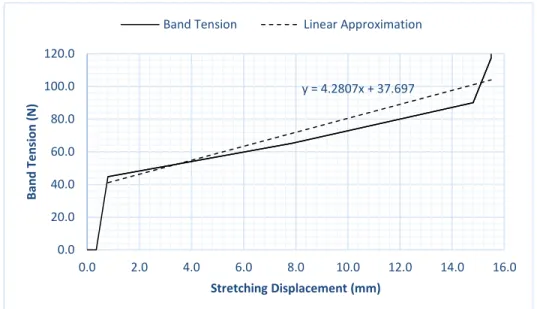
(28) 2.. Experimental Analysis. 2.1.6 ELASTIC CONSTANT AND DAMPING FACTOR First, data of tensions and lengths are collected. Then, lengths are converted into stretching in order to determine the behavior of the force exerted by the band. Finally, Excel’s linear approximation is applied to obtain the function that described the elastic constant of the band. Fig. 2.9 shows band stretch displacement and tension graph.. Band Tension 120.0. Band Tension (N). 100.0 80.0 60.0 40.0 20.0 0.0 0.0. 2.0. 4.0. 6.0. 8.0. 10.0. 12.0. 14.0. 16.0. Stretching Displacement (mm). Fig. 2.9. Tension-Stretching graph. The plot shows a rapid force grow at the beginning. Then, the function came close to linearity, with a greater slope at the end. From Fig. 2.9, the tension of the band presented a rapid increase in the first millimeters of displacement. This effect is assumed to be caused by the damping effect of real life bands, since their elastic constant is not linear. Consequently, the first two zero values are ignored for the linear approximation. The result is shown in Fig. 2.10.. 20.

(29) 2.. Band Tension. Experimental Analysis. Linear Approximation. 120.0. Band Tension (N). 100.0. y = 4.2807x + 37.697. 80.0 60.0 40.0 20.0 0.0 0.0. 2.0. 4.0. 6.0. 8.0. 10.0. 12.0. 14.0. 16.0. Stretching Displacement (mm). Fig. 2.10. The dashed line represents the linear approximation, which is described by the equation above. The linear function shown in Fig.2.10 is written as Eq. (2.38). (2.38). 𝑓(𝑥) = 𝑚𝑥 + 𝑏. Where 𝑓(𝑥) stands for the linear function, 𝑚 the slope, 𝑥 the independent variable and 𝑏 the intersection in 𝑦 -axis. For this case, 𝑓(𝑥) represents the resultant tension, 𝑚 the elastic constant, 𝑥 the respecting band length and 𝑏 the damping factor. In addition, the elastic constant is shown in Eq. (2.39).. 𝐹⃑ = −𝑘∆𝑥 → 𝑘 = −. 𝐹⃑ ∆𝑥. (2.39). Where 𝑘 stands for the elastic constant of a spring, which is negative it is opposing to the movement and ∆𝑥 is the displacement of the spring. It is worth noting that real life rubber bands have a non-linear elastic constant, which decrements during elongation due to their mechanical properties, and their capacity to transform all of the applied work into elastic potential energy is affected by heat. To compensate for this, a damper is added. The damping effect serves is velocity dependent. Consequently, the Eq. is rewritten as (2.40). 21.

(30) 2.. Experimental Analysis. ∆𝑥 𝐹⃑ = −𝑘∆𝑥 − 𝑐 ∆𝑡. (2.40). Where 𝑐 stands for the damping force over time. In summary, values of 𝑚 and 𝑏 form (2.36) correspond to 𝑘 and 𝑐 in (2.38). Therefore, the behavior of the band is described by Eq. (2.41). ∆𝑥 𝐹⃑ = −(4.3)∆𝑥 − (37.7) ∆𝑡. (2.41). The obtained elastic constant k equal to 4.3 N/mm and damping factor c equal to 37.7 Ns/mm are implemented in force-displacement numerical simulations to validate their reliability. Simplified versions of the components of the device are modelled in SolidWorks and simulated using its Motion Analyzer tool.. 2.1.7 DEVICE COMPONENTS VIRTUAL MODELLING The whole system is divided into the two components of the device, four links that substituted the cable and a poled that located the height where the cable is conducted through the socket. Fig. 2.10 shows each component and their assembly while Fig. 2.11 compares the real system against its virtual counterpart.. Fig. 2.10. 𝑎) Basic component of the device (fixed and moving). 𝑏) Link for band and cable substitution. 𝑐) Pole for height reference. 𝑑) Complete assembly.. 22.

(31) 2.. Experimental Analysis. Fig. 2.11. 𝑎) Physical device and 𝑏) Virtual mechanism. Distance from device to conducted point 284.4 mm, height relative to the rotation axis 43.3 mm. Special cases in the assembly are position relations between links. As for the user, both pairs of links that substituted the cable and the band are given position relations that makes them appear to be physically separated to the user, but the system calculations consider them as connected.. 2.1.8 FORCE-DISPLACEMENT NUMERICAL SIMULATION In order to analyze reactions and forces, a special analysis tool is activated in SolidWorks. It allows the user to add contact forces between components in the assembly, add springs, motors and external forces and to calculate the reactions, displacements and velocities. The use of such tool requires the user to select the Gear Icon in the upper menu bar and click on the “Complements…” option. Then to activate the SOLIDWORKS Motion complement. With Motion Analysis, a spring is added to emulate the behavior of the band; a linear motor simulated the force generated by the cable and collision between the moving and fixed components of the device. The parameters for the spring are 𝑘 equal to 4.3 N/mm and 𝑐 equal to 37.7 Ns/mm. For the linear motor, constant displacement of 50.0 mm at 2.5 mm/s and with its vector permanently pointing in the direction of the cable. The displacement represents the excursion of the cable. 23.

(32) 2.. Experimental Analysis. during the opening of the device. The velocity of excursion is taken directly from the test protocol of [6]. Fig. 2.12 illustrates the spring and the pulling motor.. Fig. 2.12. 𝑎) Starting position of the mechanism with the motor represented by an arrow and the spring. 𝑏) Final position of the mechanism with the maximum displacement of the spring and the motor and a difference in colors of the components due to their collision.. As seen in Fig. 2.12, the arrow keeps its pointing direction due to the design, which has the same height at the starting and ending positions, this characteristic is congruent with the physical mechanism. In addition, the second diagram illustrates the collision of the moving component against the fixed one, the stretching of the sting and its shift towards the rotation axis as it happens with the band. Table. 2.2 shows the spring and motor numerical simulation parameters. Table 2.2. Numerical simulation parameters. Motor Parameters. Spring Parameters. Time (s). 20.0. k (N/mm). 4.3. Displacement (mm). 50.0. c (Ns/mm). 37.7. The displacement of the linear motor is constrained to move in the direction of the cable in order to simulate as close as possible the path of the cable during excursion. Forces generated by the linear motor are measured against each elastic. Estimations represent the force exerted by the user. It’s worth noting, however, that SolidWorks analyzed force and displacement separately. Each of them compared against time. Whereas, the current work required a direct comparison between them. To solve such issue, estimations form SolidWorks are exported to Excel in order to proceed with deductions. 24.

(33) 2.. Experimental Analysis. First, values of displacement are inversely sorted and converted into absolute quantities. Then, the arrangement of force values is moved to fit each cell of displacement values. The result gave the tendency of the force with regard to the displacement of the cable. The resulting graph is compared to literature’s measurements, as presented in Fig. 2.13.. Simulated Cable Force. Experimental Cable Force. 30.0. Cable Force (N). 24.0 18.0 12.0 6.0 0.0 0.0. 5.0. 10.0. 15.0. 20.0. 25.0. 30.0. 35.0. 40.0. 45.0. 50.0. Excursion Displacement (mm). Fig. 2.13. Force-displacement graph comparing results from numerical simulation, solid line, and G.Smit measurements, dashed line. From Fig. 2.13, solid line represent numerical simulations results while dashed line contains literature’s experimental measurements. As seen, both lines behave almost identically, demonstrating the accuracy of the numerical simulation. It is worth noting, though, that the device used for the current work has a 50.0 mm excursion displacement limit whereas the experimental one had an excursion limit of around 46.0 mm.. 2.1.9 ACTIVATION WORK In mechanics, work is the energy transferred through force. The simplest case is the linear movement of an object when a constant force is applied; work is the product of force and parallel displacement. The moment of the force represents the perpendicular product of force and displacement. As a formula review, both products are presented in Eq. (2.42). 25.

(34) 2.. Experimental Analysis. ⃑⃑⃑⃑ = 𝐹⃑ ∙ 𝑟⃑ = |𝐹⃑ | ∙ |𝑟⃑| cos(𝜃)⁡;⁡𝜏⃑ = 𝑟⃑ × 𝐹⃑ = |𝑟⃑| ∙ |𝐹⃑ |sin⁡(𝜃) 𝑊. (2.42). When the force varies over time, which is the case of the current work, the general formula is a Line Integral, as shown in Eq. (2.43).. ⃑⃑⃑⃑ = ∫𝑟2 𝐹⃑ ∙ 𝑑𝑟⃑ 𝑊 𝑟 1. (2.43). A Line Integral considers a force varying in its magnitude and direction; therefore, it takes into account an infinite number of possibilities during the trajectory.[9] Graphic explanation is shown in Fig. 2.14. The area under the curve is the total work done by the system.. Fig. 2.14. The graph shows the irregular path of a moving force; where 𝑑𝑟⃑ stands for the derivative of the displacement and 𝐹⃑ the magnitude of the force at an specific point. For the current research, it should be referred as “Activation Work”, as it measures the energy required during the opening of the device. In addition, the units are converted into “Nmm” in order to be congruent to the data form "Efficiency of voluntary opening hand and device prosthetic devices: 24 years of development?," [27]. It is worth noting that the component of the displacement taken for the calculations is parallel to the vector of the force, which magnitude is taken from the averaged elastic constant numerical simulation.. 26.

(35) 2.. 2.2. Experimental Analysis. TEST MECHANISM DESIGN. In order to furtherly validate the reliability of the characterization methodology, four force reducers are tested. The purpose of each design is to reduce the excursion force and compare the area below the curve in each case. The first proposed designs are a single lever and an arrangement of two levers. The single lever design possesses two attachment points, one for the cable to the device and the other for the cable to the user. It is tested in two positions, at 60.0° from the horizontal axis and at 90.0°. The double lever is designed in a checkmark shape, with the shorter lever at 60.0° from the horizontal axis, with a length of 50.0 mm and the longer one at 90.0° and a length of 75.0 mm. The shorter lever is attached to the device, while the longer one is attached to the user. Activation force is simulated and its distribution analyzed for each design. The length of the shorter lever as well as the lower attachment location in the single lever proposal are designed to measure the same as the pulling arm in the device. The choice is arbitrary, in order to have the simplest starting point for the analysis. The larger section of the mechanism is 1.5 times the length of the shorter, once again an arbitrary selection. The first tests are meant to observe the ratio of reduction with respect of the increment of the pulling radius. The dimensions of the proposed lever solutions are presented in Fig. 2.15.. Fig. 2.15. 𝑎) Double lever design. 𝑏) Lever corresponding to the 60.0° position. 𝑐) Lever corresponding to the 90.0° position.. It’s worth noting that the addition of the mechanism requires two segments of cable as well as the total length is slightly increased due to height difference. Both tradeoffs are done for sake of the augmented leverage. 27.

(36) 2.. Experimental Analysis. Complete mechanism models in their initial positions are presented in Fig. 2.16.. Fig. 2.16. 𝑎) Double lever model, highest point to cable conduit distance 209.8 mm, lower point to device distance 53.4 mm. 𝑏) Single lever model at 90.0°, highest point to cable conduit distance 207.0 mm, lower point to device distance 79.7 mm. 𝑐) Single lever model at 60.0°, highest point to cable conduit distance 244.3 mm, lower point to device distance 53.9 mm. 𝑑) Original system, device to cable conduit distance 284.4 mm.. As seen in Fig. 2.16, the sum of both segments in the single lever proposals result in a cable slightly longer than the original. In contrast, the double lever solution requires slightly less cable. Lengths are compared in order to prove the significance of this aspect for the final device. Total values and their estimated percentage of difference in length are presented in Table 2.3. Table 2.3. Left column shows the lengths of the band. Right column shows the new values of force deduced. Cable Length (mm). Length Difference. Percentage of Change. Original. 284.4. 0. 0. Single Lever 90°. 286.7. 2.3. 1%. Single Lever 60°. 298.2. 13.8. 5%. Double Lever. 263.1. -21.2. -7%. As observed in Table 2.3, the values of the longer cables are roughly 5% above the original length, which, in addition to them being in the order of millimeters, made them not significant 28.

(37) 2.. Experimental Analysis. for the physical device. Ironically, the highest difference actually comes from the shortest cable, albeit its difference still is considerably low. The fourth design consists of two pulleys of different diameter mounted one over the other. The radius of the smaller one is equal to the height of the cable attachment of the device and is connected to it through a cable. While the radius of the larger pulley is equal to the length of the previous lever and is connected to the body of the user. The dimensions of the pulleys match the dimensions of the levers in order to compare their performances. The larger pulley has a radius of 75.0 mm and the smaller pulley has a radius of 43.3 mm. The pulleys are mounted one over the other to reduce the amount of area required. In addition, the cable is substituted by a chain in order to reduce the amount of redundant constrains in the numerical simulation that make unnecessary usage of computational resources. Pulleys and one link of the chain are presented in Fig. 2.17.. Fig. 2.17. 𝑎) Pulley connected to the user, radius 75.0 mm. 𝑏) Pulley attached to the device, radius 43.3 mm. 𝑐) Chain link. Protuberances in the perimeter of the pulleys are used to attach the chain links.. There are, however, two considerations taken into account. The first one is that their force vector within the cable conserves its direction during the excursion. In contrast, the lever design does cause a variation in its direction, as shown in Fig. 2.18.. 29.

(38) 2.. Experimental Analysis. Fig. 2.18. 𝑎) Lever at 90.0° initial position. 𝑏) Lever at 90.0° final position. 𝑐) Pulley system initial position. 𝑑) Pulley system final position. As demonstrated in Fig. 2.18, force vector on the pulleys does not change direction from initial to final positions, whereas it varies in the lever. Such characteristic allows the pulley to keep a constant moment of torsion. For the current work, the spring of the device causes the moment of torsion of the pulley to vary.[1] The second consideration is that the excursion displacement is larger in the pulley system than in the lever, due to the arch length caused by the angular displacement, as it is demonstrated in Eq. (2.44).. (2.44). 𝑠⃑ = 𝑟⃑∆𝜃. Where 𝑠⃑ stands for “Arch Length”, 𝑟⃑ for the radius of the pulley and ∆𝜃 for the angular displacement. For instance, the larger pulley requires an angular displacement of 63.1° in order to fully open the device. Hence, the arch length generated with a radius equal to the length of the previous levers, 75.0 mm, is 82.637. As deduced in Eqs. (2.45) and (2.46):. 𝜋. ∆𝜃 = (63.1°) (180°) = 1.1⁡𝑟𝑎𝑑. (2.45). 30.

(39) 2.. Experimental Analysis. (75.0⁡𝑚𝑚)(1.1) = 82.5⁡𝑚𝑚. (2.46). Whereas the lever located at 90.0° requires an excursion displacement of just 62.3 mm to open the device as seen in Fig. 2.18. The complete mechanism in its initial and final positions is shown in Fig. 2.19.. Fig. 2.19. Pulley complete mechanism. 𝑎) Initial position, distance from able conduit to pulley bearing 123.0 mm, distance from pulley bearing to device rotation axis 136.5 mm, distance from chain link to cable conduit 122.3 mm. 𝑏) Final position, distance from chain link to cable conduit 41.8 mm. From Fig. 2.19, the chain is modelled just for the contact instances since are required for the calculations. Ends of the chains are connected by SolidWORKS constrains.. 2.3. FORCE DISTRIBUTION AND ACTIVATION WORK ANALYSIS. The 𝑘 and c values of the spring are 4.3 N/mm and 37.7 Ns/mm for all three designs. The displacement parameter of the motor is changed in each case due to the length differences of their paths. It is worth noting, though, the importance of the increment of displacement since, according to [5], there’s a excursion tolerance where the more cable is required to be excurse, the less comfortable the prosthetic limb is to manipulate. This drawback is a consequence of physiological limitations of the user’s shoulder. Therefore, the tradeoff is that reducing excursion force increases cable displacement. Finding the equilibrium point is more important than an indefinite reduction of force. The cable length difference between the initial and final positions of the proposed mechanisms is deduced in order to validate if each of satisfy the excursion tolerance. In addition, a rate in displacement growth is calculated for further comparison with force reduction. Final position of each 31.

(40) 2.. Experimental Analysis. solution is presented in Fig. 2.20. Displacements, deduced difference and growth rate are shown in Table 2.4.. Fig. 2.20. 𝑎) Double lever, distance from lever to cable conduit 144.1 mm. 𝑏) Single lever model at 90.0°, distance from lever to cable conduit 170.0 mm. 𝑐) Single lever model at 60.0°, distance from lever to cable conduit 144.7 mm 𝑑) Original device model, distance to cable conduit 234.5 mm. Table 2.4. First column tags the original mechanisms and the proposals. Second and third columns the compare the initial and final positions of the mechanisms. Fourth column collects calculated cable excursions. Fifth column presents displacement growth in comparison to the original excursion. Initial Position (mm). Final Position (mm). Cable Excursion (mm). Displacement Growth. Device. 284.4. 234.5. 50.0. 0%. Single Lever 90°. 207.0. 144.7. 62.3. 25%. Single Lever 60°. 244.3. 169.9. 74.4. 49%. Double Lever. 209.8. 144.1. 65.7. 32%. As observed in Table 2.4, cable excursion have a significant growth, ranging from around 25% to almost 50% of the original. These results are taken into consideration, especially due to the aforementioned limitations, since it implies that at some point not all users are able to fully open the device. It is worth noting though, that most activities do not require full aperture of the device, thus, there is a window for force reduction in spite of device aperture. Additionally, activation work is the main criteria of the proposal. Therefore, reduction of peak force does not necessarily 32.

(41) 2.. Experimental Analysis. mean that the activation work of the device is reduced, since it is both force and displacement dependent. Taking into account this consideration, calculated cable excursion is later compared with activation work in order to find the sweet spot between excursion and work reduction. With regards of the simulation parameters, a highly stiff spring is added to connect the device to the lever. Figs. 2.21, 2.22 and 2.23 show the initial and final conditions of each design with the added spring.. Fig. 2.21. Double Lever Design. 𝑎) Initial position of the mechanism, shorter lever parallel to the device’s arm, added string connecting lever to device. 𝑏) Final position, no collision in the device.. It is worth noting that the absence of collision at the final position due to the design of the lever means that the device cannot reach its full aperture. However, this consideration is mostly imperceptible.. Fig. 2.22. Single Lever at 90.0° Design. 𝑎) Initial position of the mechanism, longer connecting string. 𝑏) Final position, no collision in the device.. 33.

(42) 2.. Experimental Analysis. Once again, there is no collision in the device at its final position. The difference in distance is larger than in the double lever design. Further considerations such as activation work and peak force serve to prove the quality of the proposal.. Fig. 2.23. Single Lever at 60.0° Design. 𝑎) Initial position of the mechanism, lever parallel to the device’s arm. 𝑏) Final position, collision in the device.. As observed in Fig. 2.23, the single lever at 60.0° proposal proves to be the only design that allows full aperture. In contrast, it is the design than requires the most cable excursion. Nevertheless, further considerations are taken into account to determine the best candidate for the proposal. Numerical simulations are carried out as in Chapter 1. The 𝑘 and c values of the spring are 4.3 N/mm and 37.7 Ns/mm, respectively. The displacement parameter of the motor is changed due to an increase in the excursion displacement. Once again, the importance of the increment of displacement since, according to [5], there’s an excursion tolerance where the more cable is required to be excurse, the less comfortable the prosthetic limb is to manipulate. This drawback is a consequence of physiological limitations of the user’s shoulder. Complete mechanism along with its simulation parameters are shown in Fig. 2.24.. 34.

(43) 2.. Experimental Analysis. Fig. 2.24. Pulley mechanism numerical simulation a) Initial position, whole chain in contact with larger pulley, shorter pulley attached to device by chain and spring. b) Final position, majority of the chain in contact with smaller pulley.. As seen in Fig. 2.24, a highly stiff spring connects the chain to the device in order to accurately transmit the force. Collision is detected for each link and pulley.. 35.

(44) 2.. Experimental Analysis. 36.

(45) 3.. Results. 3. RESULTS. 3.1. CHARACTERIZATION METHOD. A second order function equation is generated from force-displacement in order to approximate the curve is presented in Fig. 3.1. Simulated Cable Force. Polynomial Approximation. Cable Force (N). 30.0 24.0 y = -0.0017x2 + 0.1509x + 19.771. 18.0 12.0 6.0 0.0 0.0. 5.0. 10.0 15.0 20.0 25.0 30.0 35.0 40.0 45.0 50.0 Excursion Displacement (mm). Fig. 3.1. Dashed line represents the second order polynomial equation, which is required to deduce the total work of the system.. 37.

(46) 3.. Results. The equation presented in Fig. 3.1 is integrated in order to calculate the activation work from the original mechanism. As presented in (3.1), (3.2) and (3.3).. ⃑⃑⃑⃑ = ∫50.0(−0.0017𝑟 2 + 0.1509𝑟 + 19.771)𝑑𝑟⃑ 𝑊 0. 3. (3.1). 2. ⃑⃑⃑⃑ = −0.0017𝑟 + 0.1509𝑟 + 19.771𝑟⁡|50.0 𝑊 0 3 2. (3.2). ⃑⃑⃑⃑ = −70.8 + 188.6 + 988.6 = 1,106.3⁡𝑁𝑚𝑚 𝑊. (3.3). Total work estimated during full aperture of the system is 1,106.3 Nmm. Maximum cable tension at full aperture, tensions from the varying force measurement and total work of the system from G.Smit et al. [8] are compared against numerical simulation and calculated predictions. Errors estimations and measurements are calculated in order to validate the reliability of the method. Table 3.1 compares cable tensions and activation work measured by [8] against the estimated values from the numerical simulation present the error between measured and simulated values and the accuracy of the method to predict them. In Table 3.1, the first column tags the quantities. Measured values, simulated values, errors and percentage of accuracy are shown in the second, third, fourth and fifth columns. Table 3.1. Result validation G. Smit et al.. Numerical Simulation. Error. Accuracy. Tension at 1.7 mm (N). 20.0. 20.3. 0.0155. 98%. Tension at 20.0 mm (N). 22.0. 22.1. 0.0045. 99%. Tension at 43.5 mm (N). 23.6. 23.1. 0.0225. 98%. Tension at 46.1 mm (N). 30.0. 23.1. 0.2933. 77%. 1,128.0. 1,106.342. 0.0192. 98%. Total Work (Nmm). 38.

(47) 3.. 3.2. Results. FORCE DISTRIBUTION. Single lever proposals prove to perform better than the double lever design, which actually increases the peak excursion force up to 25.0 N. However, it does reduce the area under the curve of the force, which satisfies work reduction. Data from the estimations is exported to Excel and rearranged in order to deduce the behavior of the force with respect of the displacement. Simulated force-displacement graph for the double lever design and its third order approximation equation is shown in Fig. 3.2.. Simulated Cable Force. Polynomial Approximation. 30.0. Cable Force (N). 25.0 20.0. y = 0.0001x3 - 0.0073x2 + 0.3284x + 8.122. 15.0 10.0 5.0 0.0 0.0. 5.0. 10.0 15.0 20.0 25.0 30.0 35.0 40.0 45.0 50.0 55.0 60.0 Excursion Displacement (mm). Fig. 3.2. Force-displacement graph of the double lever design. Dashed line represents third order approximation function. The area below the curve is significantly smaller than the one from the original system.. Once again, the function equation of the curve is integrated in order to deduce the total work required by the mechanism. Deductions are presented in Eq. (3.4), (3.5) and (3.6).. ⃑⃑⃑⃑ = ∫63.0(0.0001𝑟 3 − 0.0073𝑟 2 + 0.3284𝑟 + 8.122)𝑑𝑟⃑ 𝑊 0. 4. 3. 2. (3.4). ⃑⃑⃑⃑ = 0.0001𝑟 − 0.0073𝑟 + 0.3284𝑟 + 8.122𝑟⁡|63.0 𝑊 0 4 3 2. (3.5). ⃑⃑⃑⃑ = 393.8 − 608.4 + 651.7 + 511.7 = 948.8⁡𝑁𝑚𝑚 𝑊. (3.6) 39.

(48) 3.. Results. The resulting work 948.8 Nmm is fairly lower than the original 1,106.3 Nmm even if the peak force is not. This result is further compared to validate the relevance of the design. Next, the single lever at 90.0° case is simulated. It does reduce the peak force down to 17.0 N, while having a shorter displacement than the double lever design. Peak force is already proved to be reduced. Once again, data is exported to Excel the prior process is carried out in order to deduce the total work required by the design. The resulting graph and its function equation are presented in Fig. 3.3.. Simulated Cable Force. Polynomial Approximation. 30.0. Cable Force (N). 25.0 20.0 y = 8E-05x3 - 0.006x2 + 0.2083x + 8.1309. 15.0 10.0 5.0 0.0 0.0. 5.0. 10.0 15.0 20.0 25.0 30.0 35.0 40.0 45.0 50.0 55.0 60.0 Excursion Discplacement (mm). Fig. 3.3. Force-displacement graph of the single lever at 90.0°. Force reduced to 17.0 N, behavior resembled double lever force increment with less steep slope.. Function integration is presented in Eq. (3.7), (3.8) and (3.9).. ⃑⃑⃑⃑ = ∫60.0(0.00008𝑟 3 − 0.006𝑟 2 + 0.2083𝑟 + 8.1309)𝑑𝑟⃑ 𝑊 0. 4. 3. 2. (3.7). ⃑⃑⃑⃑ = 0.00008𝑟 − 0.006𝑟 + 0.2083𝑟 + 8.1309𝑟⁡|60.0 𝑊 0 4 3 2. (3.8). ⃑⃑⃑⃑ = 259.2 − 432 + 374.9 + 487.9 = 690.0⁡𝑁𝑚𝑚 𝑊. (3.9) 40.

(49) 3.. Results. The single lever design performed better than its double lever counterpart regarding peak force, displacement and work. Then, just one design remained to be tested. Finally, the single lever at 60.0° proposal is simulated. It allows further reduction, down to 15.0 N; however, its parallel displacement increased up to 75.0 mm, which causes total work to increase considerably. Simulated Cable Force. Polynomial Approximation. 30.0. Cable Force (N). 25.0 20.0 15.0 y = -0.0005x2 + 0.0315x + 14.787. 10.0 5.0 0.0. 0.0 5.0 10.0 15.0 20.0 25.0 30.0 35.0 40.0 45.0 50.0 55.0 60.0 65.0 70.0 75.0 Excursion Displacement (mm). Fig. 3.4. Force-displacement graph. Peak force reduced to 15.0 N, behavior resembled original mechanism increment. Function equation has the steepest slope of the three.. As seen in Fig. 3.4, the function Eq. of the single lever at 60.0° presented the largest area below the curve. It is inferred that its work is the largest as well. Deductions carried out to prove it are shown in Eqs. (3.10), (3.11) and (3.12).. ⃑⃑⃑⃑ = ∫75.0(−0.0005𝑟 2 + 0.0315𝑟 + 14.787)𝑑𝑟⃑ 𝑊 0. 3. 2. (3.10). ⃑⃑⃑⃑ = −0.0005𝑟 + 0.0315𝑟 + 14.787𝑟⁡|75.0 𝑊 0 3 2. (3.11). ⃑⃑⃑⃑ = −70.3 + 88.6 + 1,109.0 = 1,127.3⁡𝑁𝑚𝑚 𝑊. (3.12). Surprisingly enough, total work estimated of the design turns out to be larger than the original. In fact, it is almost the same as the one from [8]. Such result suggests that the rate 41.

(50) 3.. Results. of reduction of peak force is compensated by the displacement growth for that position and so, it maintains the peak force for a longer distance than the other solutions. In addition, the steeper slope at the beginning means that the system reached its peak force earlier than the other designs. As it is predicted, excursion displacement increased up to 82.6 mm. Surprisingly enough, peak excursion force increased as well, estimating a value of 37.0 ± 2.0 N. Force-displacement graph along with its polynomial approximation are shown in Fig. 3.5.. Simulated Cable Force. Polynomial Approximation. 40.0 35.0. Cable Force (N). 30.0. y = 0.0033x2 - 0.5229x + 35.823. 25.0 20.0 15.0 10.0 5.0 0.0 0.0. 10.0. 20.0. 30.0. 40.0. 50.0. 60.0. 70.0. 80.0. Excursion Displacement (mm). Fig. 3.5. Force-displacement graph and polynomial equation. Pulleys excursion force decreases over time, albeit its peak value is higher than in the levers simulations. It’s worth noting that erratic values are caused by collision errors in the numerical simulation. As seen in Fig. 3.5, peak excursion force is the highest of the proposed designs and even higher than the original device. In addition, the larger excursion displacement required furtherly discards the pulleys ideal candidates. Nevertheless, its total activation work is deduced after its polynomial equation, as shown in Eqs. (3.13), (3.14), (3.15) and (3.16).. ⃑⃑⃑⃑ = ∫82.6(0.0033𝑟 2 − 0.5229𝑟 + 35.823)𝑑𝑟⃑ 𝑊 1.3. 3. 2. ⃑⃑⃑⃑ = 0.0033𝑟 − 0.5229𝑟 + 35.823𝑟⁡|82.6 𝑊 1.3 3. 2. (3.13). (3.14) 42.

(51) 3.. Results. ⃑⃑⃑⃑ = [620.8 − 1,785.5 + 2,960.4] − [0.002 − 0.428 + 45.585] 𝑊. (3.15). ⃑⃑⃑⃑ = [1,795.7] − [45.2] = 1,750.5⁡𝑁𝑚𝑚 𝑊. (3.16). Regarding activation work, pulleys performed worse. Nonetheless, there are two additional considerations according to [5] and [11]: First, cable excursion has a limit of 20% of the original device. For which the 90.0° design is the closest to the limit with 25%. The limit is significantly exceeded by the remaining two.. Cable Excursion Displacement 100.0 90.0. Excursion Displacement (mm). 80.0. 74.4 65.7. 70.0. 62.3. 60.0 49.9 50.0 40.0 30.0 20.0 10.0 0.0 Device. Double-Lever. Single-Lever 90°. Single-Lever 60°. Fig. 3.6. Chart compares cable excursion for device opening in each case. Excursion increase is perceptible. Placing the single lever at 90.0° allowed the less growth. Second, patients do not actually require to fully open their device most of the time. In fact, largest common reach up to 50.0 mm, which is slightly less than half the total excursion of the cable, since the device used for the current work has an aperture of 120.0 mm in total. In such case, the three proposals are taken into account. Consequently, a second deduction of total work is carried out with half the total displacement. Eq. (3.17), (3.18) and (3.19) deduced the new work for the double lever design. 43.

(52) 3.. ⃑⃑⃑⃑ = ∫31.5(0.0001𝑟 3 − 0.0073𝑟 2 + 0.3284𝑟 + 8.122)𝑑𝑟⃑ 𝑊 0. 4. 3. 2. Results. (3.17). ⃑⃑⃑⃑ = 0.0001𝑟 − 0.0073𝑟 + 0.3284𝑟 + 8.122𝑟⁡|31.5 𝑊 0 4 3 2. (3.18). ⃑⃑⃑⃑ = 24.6 − 76.0 + 162.9 + 255.8 = 367.3⁡𝑁𝑚𝑚 𝑊. (3.19). Eq. (3.20), (3.21) and (3.22) are used for the deduction of the single lever at 90.0° proposal.. ⃑⃑⃑⃑ = ∫30.0(0.00008𝑟 3 − 0.006𝑟 2 + 0.2083𝑟 + 8.1309)𝑑𝑟⃑ 𝑊 0. 4. 3. 2. (3.20). ⃑⃑⃑⃑ = 0.00008𝑟 − 0.006𝑟 + 0.2083𝑟 + 8.1309𝑟⁡|30.0 𝑊 0. (3.21). ⃑⃑⃑⃑ = 16.2 − 54.0 + 93.7 + 243.9 = 299.9⁡𝑁𝑚𝑚 𝑊. (3.22). 4. 3. 2. Eq. (3.23), (3.24) and (3.25) are used for the single lever at 60.0° proposal.. ⃑⃑⃑⃑ = ∫37.5(−0.0005𝑟 2 + 0.0315𝑟 + 14.787)𝑑𝑟⃑ 𝑊 0. 3. 2. (3.23). ⃑⃑⃑⃑ = −0.0005𝑟 + 0.0315𝑟 + 14.787𝑟⁡|37.5 𝑊 0 3 2. (3.24). ⃑⃑⃑⃑ = −8.8 + 22.1 + 554.5 = 567.9𝑁𝑚𝑚 𝑊. (3.25). Deduction of the original systems opened to half the excursion is carried out in order to compare the performance of the proposals. As shown in Eqs. (3.26), (3.27) and (3.28).. ⃑⃑⃑⃑ = ∫25.0(−0.0017𝑟 2 + 0.1509𝑟 + 19.771)𝑑𝑟⃑ 𝑊 0. (3.26) 44.

(53) 3.. 3. 2. Results. ⃑⃑⃑⃑ = −0.0017𝑟 + 0.1509𝑟 + 19.771𝑟⁡|25.0 𝑊 0. (3.27). ⃑⃑⃑⃑ = −8.9 + 47.2 + 494.3 = 532.6⁡𝑁𝑚𝑚 𝑊. (3.28). 3. 2. Pulley’s half excursion work is also estimated, as presented in Eqs. (3.29), (3.30), (3.31) and (3.32).. ⃑⃑⃑⃑ = ∫41.3(0.0033𝑟 2 − 0.5229𝑟 + 35.823)𝑑𝑟⃑ 𝑊 1.3. 3. 2. (3.29). ⃑⃑⃑⃑ = 0.0033𝑟 − 0.5229𝑟 + 35.823𝑟⁡|41.3 𝑊 1.3. (3.30). ⃑⃑⃑⃑ = [77.6 − 446.4 + 1,480.2] − [0.002 − 0.428 + 45.585] 𝑊. (3.31). ⃑⃑⃑⃑ = [1,111.4] − [45.1] = 1,066.3⁡𝑁𝑚𝑚 𝑊. (3.32). 3. 2. 3.2.1 LEVER’S COMPARISON Estimations are collected and compared in order to support the reliability of the selection. Figs. 3.7 and 3.8 show the column charts comparing work and cable excursion respectively.. 45.

(54) 3.. Results. Full Excursion Work 1,600.0 1,400.0. Activation Work (Nmm). 1,200.0. 1,127.3. 1,106.3 948.8. 1,000.0 800.0. 690.0. 600.0 400.0 200.0 0.0 Device. Double-Lever. Single-Lever 90°. Single-Lever 60°. Fig. 3.7. Chart compares activation work required for the system in each case. As illustrated, work is reduced significantly by locating the single lever at 90.0°. As seen in the charts, the single lever at 90.0° proposal proves to perform the most work reduction and added the least excursion displacement.. Half Excursion Work 800.0. Activation Work (Nmm). 700.0 600.0. 567.9. 532.6. 500.0 367.3. 400.0. 299.9 300.0 200.0 100.0 0.0 Device. Double-Lever. Single-Lever 90°. Single-Lever 60°. Fig. 3.8. Chart compares work required for opening half the system’s aperture in each case. Once again, work is reduced significantly by locating the single lever at 90.0°. 46.

(55) 3.. Results. From Fig. 3.7 and 3.8, the single lever at 90.0° proposal demonstrates the best performance. Percentage of work reductions are deduced for both the full and half excursion cases in order to further validate the performance of the 90.0° lever. As it is shown in Table 3.2: First column tags the original mechanism and the proposals. Second column compares total work in each system. Third column collects work reduction percentages from each proposal to the original device. Fourth column compares work done at half the total cable excursion. Fifth column collects second work reduction percentages. From Table 3.2, single lever at 90.0° proposal demonstrates the most activation work reduction in both tests. It actually performed better at half excursion with 44% and 38% at full. Interestingly enough, placing the lever at 60.0° actually increased the activation work, as it is expressed with 0%. Table 3.2. Activation works and reduction percentages. Full Excursion Work (Nmm). Work Reduction Percentage. Half Excursion Work (Nmm). Work Reduction Percentage. Device. 1,106.3. 0%. 532.6. 0%. Double Lever. 948.8. 14%. 367.3. 31%. Single Lever at 90.0°. 690.0. 38%. 299.9. 44%. Single Lever at 60.0°. 1,127.3. 0%. 567.9. 0%. Furthermore, the 90.0° proposal adds the least cable displacement of the three, with a 25% of extra excursion. For which it is chosen as the proposal’s mechanism during the first stage of the work. Fig. 3.9 presents a comparative chart of both half and full excursion activation works. Fig. 3.10 compares their respective reduction percentages.. 47.

(56) 3.. Full Excursion Work. Results. Half Excursion Work. 1,600.0 1,400.0. Activation Work (Nmm). 1,200.0. 1,127.3. 1,106.3 948.8. 1,000.0 800.0 600.0. 690.0 567.9. 532.6 367.3. 400.0. 299.9. 200.0 0.0 Device. Double-Lever. Single-Lever 90°. Single-Lever 60°. Fig. 3.9. Chart compares activation work for both half and full device aperture. Single lever at 90.0° proposal has perceptibly the lowest activation work.. Half Excursion Work Reduction. Full Excursion Work Reduction. 100%. Activation Work Reduction (%). 90% 80% 70% 60% 50%. 44% 38%. 40% 31% 30% 20%. 14%. 10% 0%. 0%. 0% Double-Lever. Single-Lever 90°. Single-Lever 60°. Fig. 3.10. Chart compares activation work reduction for both half and full device aperture. Once again, single lever at 90° proposal demonstrates the highest reduction performance. With a higher reduction percentage at half excursion. 48.

(57) 3.. Results. 3.2.2 PULLEY AND LEVER COMPARISON Values are collected and compared against the lever at 90.0° ones. Chart shown in Fig. 3.20 compares activation works at full excursion displacement. From Fig. 3.10, differences between activation works are abysmal, as pulley’s work is more than double the value of the lever. In addition, chart in Fig. 3.12 shows activation works at half excursion displacements. As seen in Fig. 3.11, pulleys perform worse in the first half of the device opening, which is reasonable due to the high peak force at the beginning.. Full Excursion Work 2,400.0 2,200.0 2,000.0. Activation Work (Nmm). 1,800.0. 1,750.5. 1,600.0 1,400.0 1,200.0 1,000.0 690.0. 800.0 600.0 400.0 200.0 0.0 Pulleys. Single-Lever 90°. Fig. 3.11. Chart compares full excursion activation works. Pulley work is significantly greater.. 49.

(58) 3.. Results. Half Excursion Work 1,600.0. Activation Work (Nmm). 1,400.0 1,200.0. 1,066.3. 1,000.0 800.0 600.0 400.0. 299.9. 200.0 0.0 Pulleys. Single-Lever 90.0°. Fig. 3.12. Half excursion work comparison chart. The gap between activation works is larger than in the full excursion case.. Results of both full and half excursion activation work prove the pulleys to be inefficient. In both cases and furthermore, in the initial stage of the opening, the lever design allows the user to require 72% less activation work. Comparison chart for both full and half excursion woks is shown in Fig. 3.22.. 50.