Chapter I
Confidence Interval and
Sampling
... ....
…...
Objetive
Chapter
1.1 Introducción
Estimation techniques are used when the researcher has no prior assumptions about the value of a population characteristic and want to know what that value might be.
Statistical inference contains two types of procedures regarding universal parameters, made on the basis of sample evidence.
The procedures are: Parameter estimation and Hypothesis.
The estimation assumes two forms: - Point estimates
- Estimates by interval
1.2 Point Estimates
Is a single value (point) derived from a sample and used to estimate a population value. For example, suppose we select a sample of 30 executives of Kigali Bank and ask each the number of hours they worked last week. Compute of this sample of 30 and use the value of the sample mean as a point estimate of the unknown population mean. However, a point estimate is a single value, for more informative approach is to present a range of values (confidence interval) in which we expect the population parameter to occur.
One Sample
Two Samples
1.3 Confidence Interval
A range of values constructed from a sample data so that the population parameter is likely to occur within the range at a specified probability. The specified probability is called the level of confidence.
How to Interpret Confidence Intervals
The confidence level describes the uncertainty associated with a sampling method. Suppose we used the same sampling method to select different samples and to compute a different interval estimate for each sample. Some interval estimates would include the true population parameter and some would not. For 95% confidence interval indicates the range of values within which the true value will fall 95% of the time. That is we are likely to be wrong only 5% of the time.
p P s
x
, ˆ , ˆ
ˆ 2 2
2 1 2 1 ˆ
ˆ x x s s 2 2 2 1 2 2 1 2 2 2 2 1 ˆ ˆ
Confidence Interval Data Requirements
To express a confidence interval, you need three pieces of information. Statistic
Confidence level Margin of error
Often, the margin of error is not given; you must calculate it.
There are three steps to constructing a confidence interval:
1. Identify a sample statistic. Choose the statistic (e.g. sample mean, sample proportion) that you will use to estimate a population parameter; according to type of variable (e.g. mean if the variable is numerical or proportion if the variable is categorical).
2. Select a confidence level. The confidence level is the probability value associated with a confidence interval. It is often expressed as a percentage. For example, say, then the confidence level is equal to (1-0.05) = 0.95, i.e. a 95% confidence level. Often, researchers choose 90%, 95%, or 99% confidence levels; but any percentage can be used.
3. Find the margin of error. To calculate the margin of error, follow the following equation: Margin of error = Probability value * Standard error of mean
Standard error of mean =
The probability value comes from the critical value provided by the probability distribution according to the level of confidence.
1.3.1 Confidence interval for a mean when the population standard deviation is unknown
A confidence interval for a mean specifies a range of values within which the unknown population parameter may be lie, in this case the mean. These intervals can be calculated for: if an employer wishes to estimate the average daily sale; a producer who wants to estimate his average daily production; a medical researcher who wants to estimate the average response of patients to a new medication; etc. Also the confidence intervals are widely used in the quality control of products.
One of the most used probability distributions is "Student's t distribution" this must be used to find areas under the sampling distribution and establish the critical region. When we use "t" you need to know what degree of freedom is.
Degrees of Freedom
The degrees of freedom refer to the number of independent observations in a set of data.
When estimating a mean score or a proportion from a single sample, the number of independent observations is equal to the sample size minus one (n-1 = df). Hence, the distribution of the t statistic from samples of size 26 would be described by a t distribution having 26-1 or 25 degrees of freedom. Similarly, a t distribution having 15 degrees of freedom would be used with a sample of size 16.
In practice, rule rather than exception is the fact that the standard deviation of the population is unknown. Gosset, who wrote under the pseudonym Student described the following formula:
Note: For this method to be valid it is very important that the population be normal, that is, if the population is skewed or has outliers the calculation below will yield an inaccurate confidence interval. The reason that we need normality here is that “n” being less than 30 is too small for the Central Limit Theorem to do its magic of making the sample mean nearly normal.
Example 1:
Rongin Kwizera is the host of the news of KXYZ Radio 55 AM in kigali. During his morning program, Rongin asks listeners to call in and discuss current local and national news. This morning, Rongin was concerned about the number of hours that children under 12 years watch TV per day. The last 5 callers reported that their children watched the following number of TV hours on the last day.
Data from Sample of callers: 1.0, 2.3, 3.1, 0.30, 3.5
Would it be reasonable to develop a confidence interval from these data to show the mean number of hours of TV watched? If yes, construct and appropriate confidence interval at 95% of confidence, and interpret the result.
If no, why would a confidence interval not be appropriate? Solution:
Mean= 2.04
Std. Deviation= 1.36
t distribution for df of 4= 2.776
Answer: 0.35 < u <3.73
Interpretation: At 95% of confidence the children under 12 years of ages watches TV between 0.35 to 3.73 hours per day. See: in this example requires that the variable is normally distributed.
Find the probability value in Excel: Open excel and look for the insert function icon (fx) > select a category > select Statistical > select a function TINV > OK > after that follow the picture
Steps in SPSS for Confidence Interval for One Sample t Test
First create the variable in (Variable View), and then fill in the data in (Data View) and third Analyze.
Analyze > Compare Means > One sample T test > Double-click Hours to move it to the Test variable (s) > Click OK. The output is displayed in the Output window.
Output of SPSS for Confidence Interval for One Sample t Test
One-Sample Statistics
N Mean
Std. Deviation
Std. Error Mean Number of hours children
under 12 years watches
TV per day 5 2.0400 1.36308 .60959
The average hours that children under 12 year old watch TV is 2.04 hours per day, and the variability between mean is 1.36, it is a heterogeneous group because CV=66.8% of variability
One-Sample Test
Test Value = 0
t df
Sig. (2-tailed)
Mean Difference
95% Confidence Interval of the
Difference Lower Upper Number of hours
children under 12 years watches TV per day
3.347 4 .029 2.04000 .3475 3.7325
At 95% of confidence the children in Kigali under 12 years old watch TV between 0.35 to 3.73 hours per day. (It is the same answer when we used formula before)
Example 2:
44 6 53 27 38 31 15 42 26 21 8 41 27 22 22 7 26 8 11 36
The sample standard deviation is 13.79 gallons and average is 25.55 gallons. Calculate the confidence interval at the 95% confidence level.
Solution
We have the following information:
= 25.55, s=13.79, n=20, and the confidence level = 95%. With a confidence level of 95% and with a sample size of 20, α is .05 and the degrees of freedom are 19. Thus form the table of “t” under the 19 df and .05 (2-tails) = 2.093 (see in Excel), the CI computed as a follow:
The formula is:
; then the CI is:
So Aphrodice can be 95% confident that the mean amount of the product sold per day is between 19.10 and 32.00 gallons.
Output of SPSS for Confidence Interval for One Sample t Test
Analyze > Compare Means > One sample T test > Double-click Gallons to move it to the Test variable (s) > Click OK. The output is displayed in the Output window.
One-Sample Statistics
N Mean Std. Deviation Std. Error Mean
Gallons 20 25.55 13.790 3.083
We see the same result on the previous example
1.3.2 Confidence Interval for Sample Proportion
X is a binomial variable of parameters n and p (a binomial variable is the number of successes in n trials, in each trial the probability of success (p) are the same), for example: The director of Business administration reports that the 40% of its graduates enter the job market in a position related to their field of study.
Note: If the sample is large and p is close to 0 or 1 (np 5) X is approximately normal with mean np and variance npq (where q = 1 - p) and can use the statistical (sampling rate), which is also approximately normal with a standard error given by
therefore a CI for p is:
)
Where:
p is a proportion q= 1-p
Proportion. The fraction, ratio, or percent indicating the part of the sample or the population having a particular trait of interest.
Note that to build it, you need to know p!. If n is large (> 30) can be replaced by their estimates p and q without much error, in any case as , then if is replaced by 0.25 yields a more conservative range (larger).
A high school counselor is interested in the percentage of male students who would volunteer for military service. He randomly samples 50 male students and finds that 15 of them would like to enlist. Use a 99 percent confidence level to estimate the true percentage. (Where 1 means they want to go to serve and "o" means they do not want to go to military service)
Data:
0 1 1 0 1 0 1 0 0 1 0 1 0 1 1 0 0 0 0 0 0 1 0 0 0
1 0 0 0 0 0 0 1 0 0 0 1 0 0 1 0 0 0 0 1 0 0 0 1 0
Solution
The data are p=15/50 = 0.30 n= 50
Confidence level = 99 percent, then t(.01, 49) = 2.68
), them the CI is
So the counselor can be 99 percent confident that the percentage of male students who would volunteer for military service is between 13 and 47 percent. (You’ll notice that this estimate may not be of much help to the counselor. Its large width results from the high level of confidence specified and the relatively small sample size.)
Output of SPSS for Confidence Interval for One Sample t Test
Analyze > Compare Means > One sample T test > Double-click students who wants to go to military service (Example 3) to move it to the Test variable (s) > Click OK. The output is displayed in the Output window.
One-Sample Test
Test Value = 0
t df Sig. (2-tailed) Mean Difference
99% Confidence Interval of the Difference
Lower Upper
Students volunteer for military
service 4.583 49 .000 .300 .12 .48
1.4 Sampling: Non Probability and Probability Samples
Planning
• Which variables will you collect and how will they be measured? • What types of data do they represent?
• What do you want to do? Describe, compare groups, and predict change in Y following change in X? • How large a sample do you need?
The concept of “representativeness” means that the selected sample of households reasonably represents the entire group (one part from each province). In addition, each household must have an equal chance of being selected to participate in the survey.
Why use a sample
Lest Cost
Less field time
Speed
Accuracy
Destruction of test units
When it’s impossible to study the whole population
Note: Homogeneous populations – small samples are highly representative
Sample accuracy, refers to how close a random sample’s statistic (e.g. mean ( ), variance (s2), proportion ( ) is to the population’s
value it represents (µ, σ2, π). Sample size, however, is related to accuracy. How close the sample statistic is to the actual
population parameter (e.g. sample mean vs. population mean is a function of sample size).
Sampling design: Steps
1. Definition of target population (Who or which is the focus in your study) Who has the information/data you need?
How do you define your target population? - Geography (like province, sector, etc.)
- Demographics (like gender, economic situation, etc.) - Use (it depends on the researcher)
- Awareness (knowledge or perception of a situation or fact.) 2. Selection of a sampling frame (list)
- List of elements
- Sampling Frame Error: error that occurs when certain sample elements are not listed or available and are not represented in the sampling frame
3. Take a decision for Probability or Nonprobability Sampling
Probability Sample:
A sampling technique in which every member of the population will have a known probability, other than zero of being selected.
Non-Probability Sample:
• Units of the sample are chosen on the basis of personal judgment or convenience.
• There are NO statistical techniques for measuring random sampling error in a non-probability sample. Therefore, generalizability is never statistically appropriate.
4. Sampling Unit. It is necessary to decide a sampling unit before selecting a sample. It can be a geographical one (state, district, village, etc.), a construction unit (house, flat, etc.), a social unit (family, club, school, etc.), or an individual.
5. Error
- Random sampling error (chance fluctuations) - Nonsampling error (design errors)
6. Sample Type. The researcher, decides the techniques to be used in selecting the items for the sample according of the characteristics of the population
7. Determination of levels of inference. We desire that our results be repeated within some known range if we were to conduct the study again.
8. Calculation the size of the sample. This is the number of items, selected from the universe, constituting a sample. The sample size should not be too large or too small, it depend of the variability od the data.
1.5 Sample Size Formula
The formula requires that we
1. Specify the amount of level of confidence we wish to have, i.e. how certain you want to be that the population figure is within the sample estimate and its associated precision.
2. Variability in the population: results from previous studies or conduct a pilot study, if the most important variable you study is quantitative, you use standard deviation, it is the most usual measure and often needs to be estimated, as well as if you estimate variable qualitative you use for variability “p” proportion; refers to how similar or dissimilar responses are to a given question P (%): share that “have” or “are” or “will do” etc. Q (%): 100%-P%, share of “have nots” or “are nots” etc. Expect the worst case (p=50%; q=50%)
N.B.: The more variability in the population being studied, the larger the sample size needed to achieve stated accuracy level. 3. Margin of error or precision, a measure of the possible difference between the sample estimate and the actual population value. 4. Population size, total number of items in the population, if the total population was not known, formulas can be used where this
total is not required.
1.5.1 The sample size formula for estimating a proportion (also called a percentage or share)
Infinite population (when the size of the population is unknown) Finite population (population size is known)
Where:
n Sample size N Population size 1-α ConfidenceZ Normal probability value associated with the chosen level ofconfidence
p
Proportion of elements that have the attributes that you are looking for
q 1-p
e Acceptable sample error
How to estimate variability “p” in the population
• Estimate variability “p”: results of previous studies or conduct a pilot study • Expect the worst case (p=50%; q=50%)
How to determine the amount of desired sample error
• Researchers should work with managers to make this decision. How much error is the manager willing to tolerate (less error = more accuracy)
• Convention is + 5%
How to decide on the level of confidence desired
• Researchers should work with managers to make this decision. The higher the desired confidence level, the larger the sample size needed
• Convention is 95% confidence level (Zα/2 =1.96)
• The more important the decision, the more likely the manager will want more confidence. For example, a 99% confidence level has a Zα/2 =2.58.
Additional correction for sampling finite populations
The above formula assumes that the population is very large compared to the proportion of the population that is sampled. If you are sampling more than 10% of the whole population then you should apply a correction to the sample size estimate that incorporates the finite population correction factor (FPC). This will reduce the sample size.
Example
We’d like to know the level of satisfaction of AUCA's students about the methodology used by teachers. The Registration office has 2800 students registered in 2016-II semester. We need to take a sample with 95% of confidence and 5% error of estimation. We need to take a sample with 95% of confidence and 5% error of estimation.
Solution Data:
N=2800 students e=0.05 (5%)
95% of confidence= (Zα/2=1.96)
At 95 percent of confidence, we should take a sample of 302 students
1.5.2 The sample size formula for estimating Mean
Infinite population Finite population
Zα/2 is determined the same way (1.96 or 2.58)
Error (e) is expressed in terms of the units we are estimating, i.e. if we are measuring attitudes on a 1-7 scale, we may want our error to be no more than + .5 scale units. If we are estimating dollars being paid for a product, we may want our error to be no more than + $3.00.
σ is a little more difficult to estimate, but must be in same units as “error”.
Estimating “ σ ” in the formula to determine the Sample Size required to estimate a Mean
Since we are estimating a mean, we can assume that our data are either interval or ratio. When we have interval or ratio data, the standard deviation of the sample, may be used as a measure of variance.
How to estimate σ?
• Use standard deviation of the sample from a previous study on the target population • Conduct a pilot study of a few members of the target population and calculate “s”
Example
An accounting firm wishes to form a 90 percent confidence interval for the population mean tax refund for its clients who receive refunds. How large a random sample is needed to be within $6 of the actual amount, if a preliminary study finds the standard deviation to be $42.67?
Solution Data:
90% of confidence (Zα/2=1.64)
e=$6 s=$42.67
With a 95 percent of confidence, the accounting firm needs a sample of 136 clients for know the tax refund.
Example
Suppose you are planning to sample transportation employees to determine average annual sick days. The following standard has been set: a confidence level of 99% and an error of fewer than 2 days. Past research has indicated the standard deviation should be 6 days. What is the required sample size?
Solution:
Sample size n ?
Confidence 1-α 0.99
Standard error associated with the chosen
level of confidence Z=Z(1- α/2) 2.58
Standard deviation ( ) 6
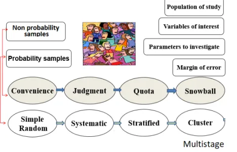
1.6 Classification Sampling Methods
Sampling method refers to the rules and procedures by which some elements of thepopulation are included in the simple. There are two methods: probabilistic sampling and non-probabilistic sampling, as shown in the following figure:
1.6.1 Probability Samples
Probability sampling is a sampling technique wherein the samples are gathered in a process that gives all the individuals in the population equal chances of being selected.
Simple Random Sampling
A method for choosing cases from a population by which every case and every combination of cases has an equal chance of being included, i.e. must be you have a homogeneous population. To use this technique, we need a list of all elements and cases are often selected by using tables of random numbers. These tables are list of numbers that have no pattern (that is, they are a random), and an example of such a table is bellow
Table of Random Numbers. The following figure shows a small part of the random table
o The purest form of probability sampling.
o Assures each element in the population has an equal chance of being included in the sample o Random number generators
Methods for use Table of Random Numbers
To use this type of sampling, it is important that the population is homogeneous, so that everyone has the same probability of appearing to reach the desired sample size.
It can be done on the basis of lists of people in the population or people who are chosen at random with a computer.
Steps:
1. List the cases to be randomized in a column on a spreadsheet.
3. To select a sample, select the desired number for the sample from either the highest or lowest assigned random numbers. For example, for N=10, choose the names with the 10 lowest random numbers.
Example
Suppose that we have a population of 48 college students and want to form a simple random sample of size five to survey about some issues on campus. We begin by assigning numbers to each of our students. Since there are a total of 48 students, and 48 is a two digit number, every individual in the population is assigned a two digit number beginning 01, 02, 03, . . . 46, 47, 48.
Answer;
The sample size is 5, and the students are:
Hellene H, Lucille L., Gilles D., Flienne M. and Alain M.
Systematic sampling
Systematic sampling requires a homogeneous population and that the population is enumerating or coding and then selecting the sample elements at regular intervals through that ordered list. Systematic sampling implies a random start and then continues with the selection of each element k from that moment. In this case, k = (size of the population / sample size). It is important that the starting point is not automatically the first in the list, but that the first element is chosen at random from the k-th in the list.
(Probability of Selection) K = population size / sample size Steps
1. The first thing you do is pick an integer that which is the result given the formula of probability of selection; this will be your first subject e.g. (3).
2. Select values systematically jumping every 3 values, so on until the required sample size.
Example
Assuming you have a population of 1,500 people and your sample size is 100. Then Kth position will be given by: N/n = 1500/100 = 15. It means that every 15th position or interval is automatically selected as part of the sample. Thus, numbers 15, 30, 45, 60, etc. are already selected.
You can even select any number: 1, 2, 3, …,15 as the Kth number. For example, if the Kth case is 5, then 5, 20, 35, 50, etc. become members of the sample
Stratified Sampling (the population is not homogeneous)
When the population is divided into different categories, the framework can be organized by these categories into separate "strata". Then, each stratum is sampled as an independent subpopulation, from which individual elements can be randomly selected. Benefits for stratified sampling
First, dividing the population into separate and independent strata may allow researchers to draw inferences about specific subgroups that may be lost in a more generalized random sample.
In a stratified sampling design, the steps we will be, first, to establish on the basis that we attribute to stratify, secondly, few variables that define attribute occur in the population and, therefore, on how many groups or strata divide the population, (the following figure shows a stratified sampling design with 4 strata, L = 4). Once determined subgroups, the next step will consist in knowing the total population belonging to each stratum (N1, N2, N3. N4) and, finally, we take a random sample from each strata we
have (n1, n2, n3, n4). The sum of the subsamples constitute the total sample (n1 + n2 + n3 + n4 = n).
Source: Stratified by Rosa Padilla. Sampling for research on environmental care in the Adventist University of Central Africa
Cluster Sampling (the population is not homogeneous)
The primary sampling unit is not the individual element, but a large cluster of elements. Either the cluster is randomly selected or the elements within are randomly selected.
Sometimes it is more cost-effective to select respondents in groups ('clusters'). Sampling is often clustered by geography, or by time periods. (Nearly all samples are in some sense 'clustered' in time, for example if surveying households within a city, we might choose to select 100 city blocks and then interview every household within the selected blocks.
We don't need a sampling frame listing all elements in the target population. Instead, clusters can be chosen from a cluster-level frame, with an element-level frame created only for the selected clusters. In the example above, the sample only requires a block-level city map for initial selections, and then a household-block-level map of the 100 selected blocks, rather than a household-block-level map of the whole city.
Cluster sampling is commonly implemented as multistage sampling. This is a complex form of cluster sampling in which two or more levels of units are embedded one in the other. The first stage consists of constructing the clusters that will be used to sample from. In the second stage, a sample of primary units is randomly selected from each cluster (rather than using all units contained in all selected clusters). In following stages, in each of those selected clusters, additional samples of units are selected, and so on. All ultimate units (individuals, for instance) selected at the last step of this procedure are then surveyed. This technique, thus, is essentially the process of taking random subsamples of preceding random samples.
Example
Other example for Cluster
Types of Cluster Samples
Area sample:
Multistage area sample:
Involves a combination of two or more types of probability sampling techniques. Typically, progressively smaller geographical areas are randomly selected in a series of steps
1.6.2 Non Probability Samples
Non-probability samples are less desirable than probability samples, because they are not truly representative, however, a researcher may not be able to obtain a random or stratified sample, or it may be too expensive. A researcher may not care about generalizing to a larger population. The validity of non-probability samples can be increased by trying to approximate random selection, and by eliminating as many sources of bias as possible.
2
Convenience Sampling
Or accidental sampling is a type of nonprobability sampling which involves the sample being drawn from that part of the population which is close to hand. That is, a population is selected because it is readily available and convenient. It may be through meeting the person or including a person in the sample when one meets them or chosen by finding them through technological means such as the internet or through phone. The researcher using such a sample cannot scientifically make generalizations about the total population from this sample because it would not be representative enough. For example, if the interviewer were to conduct such a survey at a shopping center early in the morning on a given day, the people that he/she could interview would be limited to those given there at that given time, which would not represent the views of other members of society in such an area, if the survey were to be conducted at different times of day and several times per week. This type of sampling is most useful for pilot testing.
Judgment or Purposive Sample
The sampling procedure in which an experienced researcher selects the sample based on some appropriate characteristic of sample members… to serve a purpose.
Quota sampling
In quota sampling, the population is first segmented into mutually exclusive sub-groups, just as in stratified sampling. Then judgment is used to select the subjects or units from each segment based on a specified proportion. For example, an interviewer may be told to sample 200 females and 300 males between the age of 45 and 60.
It is this second step which makes the technique one of non-probability sampling. In quota sampling the selection of the sample is non-random. For example interviewers might be tempted to interview those who look most helpful. The problem is that these samples may be biased because not everyone gets a chance of selection. This random element is its greatest weakness and quota versus probability has been a matter of controversy for several years.
Other example
For example, a television in Rwanda may be assigned 50 interviews, 20 of which are with small business owners, 18 with professionals, 12 with managerial employees, 5 supervisors, and the rest with hourly employees. Therefore the various interview quotas representing the proportion of the subgroups.
Snowball Sampling
In sociology and statistics research, snowball sampling (or chain sampling, chain-referral sampling, referral sampling) is a non-probability sampling technique where existing study subjects recruit future subjects from among their acquaintances. Thus the sample group appears to grow like a rolling snowball. This sampling technique is often used in hidden populations which are difficult for researchers to access; example populations would be drug users or sex workers. As sample members are not selected from a sampling frame, snowball samples, are subject to numerous biases. For example, people who have many friends are more likely to be recruited into the sample.
Method:
1. Draft up a participation program (likely to be subject to change, but indicative). 2. Approach stakeholders and ask for contacts.
3. Gain contacts and ask them to participate.
4. Community issues groups may emerge that can be included in the participation program. 5. Continue the snowballing with contacts to gain more stakeholders if necessary.
ASSIGNMENT 1
Multiple choices
1. Inferential statistics…
a. is the same as descriptive statistics
b. refers to the statistical methods used to draw inferences about a population based on sample information
c. is the same as a census
d. refers to the process of drawing inferences about the sample based on the characteristics of the population
e. None of the above answers is correct.
2. List three reasons to study Inferential Statistics 3. List three applications of Statistics in Business.
4. A survey found that waiting time in minutes
for 16
new customer in bank of Kigali in Rwanda in the
present year is:
12 20 28 22 24 31 32 41 35 32
33 36 40 35 43 44
Do you need to assume that the population of the new customer in bank is normally distributed to construct the confidence interval estimate for the mean of “waiting time”? Explain. Mean = 31.75, Sd= 8.83
The t distribution assumes that the variable being studied is normally distributed. The assumption of normality in the population can be assessed by evaluating the shape of the simple data using a histogram, boxplot, or normal probability plot. (Interpret graph Boxplot)
Answer: <27.05≤µ≤36.45>
5. Let 12.3, 10.5, 11.3, 12.8, 9.6, 5.3 and 8.4 the times in seconds needed for downloading 7 files on your computer from a course website. If we assume that this sample we selected from a normal distribution, construct a 95% confidence interval for the population mean µ. Answer: <7.64≤µ≤12.41>
6. Angelique is the “Cookie Lady” She bakes and sells cookies at location in Gasabo. She is concerned about absenteeism among her workers. The information bellow reports the number of days absent for a sample
of 10
workers during the last two-week pay period.
4 1 2 2 1 2 2 1 0 3
a. Develop a 99% confidence interval for the population men. Assume that the population distribution is normal. Answer: <.63≤µ≤2.97>
b. Explain why the t distribution is used as a part of the confidence interval
7. A marketing firm plans to study the annual sales in coffee shops. They want to estimate the mean annual sales to within $0.2 million, this time with 90% confidence. How many coffee shops should they sample to obtain a margin of error of at most $0.2 million with a confidence level of 90%? From a previous study they assume that the σ ≈ $1.03 million.
Answer: n= 71 (they need 71 observations such that the margin of error is 0.2 million.)
8. The Ministry of Economy places each of its employees on one of four salary scales, A, B, C and D. The number of employees on each scale is listed below: How many employees from each scale should be included in a sample of size, with a 95% confidence interval and a maximum sampling error of 5 %.
A 700 B 675 C 145 D 65
Answer: n= 309 (A=137, B=132, C=28, and D=13)
9. A company places each of its employees on one of three salary scales, A, B, and C. The number of employees on each scale is listed below: How many people from each scale should be included in a sample of size, with a 99% confidence interval and a maximum sampling error of 1 %.
A 330
B 575
C 445
Answer: n=1249 (A=305, B=532, C=412)
10. A firm employs numbers of staff in one of three categories listed below:
10 managers 34 secretaries
204 production workers.
How many managers and secretaries, and production workers did it contain?
You take a sample from each stratum, with a 90% confidence interval and a maximum sampling error of 7%. Answer:n=89(Managers = 4, Secretaries = 12, Production Workers =73).
11. We’ve just started a new educational TV program that teaches viewers all about research methods!!
We know from past educational TV programs that such a program would likely capture 2 out of 10 viewers on a typical night.
Let’s say we want to be 95% confident that our obtained sample proportion of viewers will differ from the true population proportions by not more than 5%.
up to 4 is to be accepted. How many subjects should be included in this study at 90% level of confidence? Answer: n= 356
13. Management wants to know customers’ level of satisfaction with their service. They propose conducting a survey and asking for satisfaction on a scale from 1 to 10 (since there are 10 possible answers, the range = 10). Management wants to be 95% confident in the results (95 chances in 100 that true value is captured) and they do not want the allowed error to be more than + .5 scale points. Standard deviation (S = 1.7, from a pilot study). What is n? Answer: n= 77
14. Suppose the President of health of Rwanda wants an estimate of the proportion of the population who support his current police towards revisions in the health care system. The president wants the estimate to be within 5% of the true proportion. Assume a 95% level of confidence. The president’s political advisor estimated the proportion supporting the current policy to be .70.