H 2 molecule in strong magnetic fields

Texto completo

(1)H2 MOLECULE IN STRONG MAGNETIC FIELDS M. BEAU1 , R. BENGURIA2 , R. BRUMMELHUIS3 , P. DUCLOS4. Abstract. The Pauli-Hamiltonian of a molecule with fixed nuclei in a strong constant magnetic field is asymptotic, in norm-resolvent sense, to an effective Hamiltonian which has the form of a multi-particle Schrödinger operator with interactions given by one-dimensional δ-potentials. We study this effective Hamiltonian in the case of the H2 -molecule and establish existence of the ground state. We also show that the inter-nuclear equilibrium distance tends to 0 as the field-strength tends to infinity.. 1. Introduction In the final decade before his untimely death, Pierre Duclos embarked upon a large–scale systematic study of atoms and molecules in strong homogeneous magnetic fields. This topic had already received considerable attention in the astrophysics and mathematical physics community (see for example [AtMol], [La], [NeuSt] and [LSY]). The published record of Pierre’s involvement started with the paper [BD1] (which can to a large measure be accredited to him), which established the norm-resolvent convergence, as the magnetic field strength tends to infinity, of the Pauli Hamiltonian of a non-relativistic atom in a constant magnetic field to an effective Hamiltonian describing a one-dimensional atom with the electrostatic interaction replaced by Dirac δ point-interactions. Though there exists a long and respected tradition in theoretical physics and chemistry of using Hamiltonians with δ-potentials as toy models (going back, at least, to the Kronig and Penney model of solid state physics), this theorem gave an example of such δ-potentials naturally arising as part of a genuine physical problem. Around the same time, [BaSoY] proved by a different method that the ground-state energy of the true Hamiltonian converges to that of the corresponding δ-Hamiltonian. The Hartree functional associated to the δ-Hamiltonian had already made its appearance in [LSY]. The approach initiated in [BD1] was further developed in [BD3], which established a three-member hierarchy of effective multi-particle Hamiltonians on the line, each one of which is asymptotic, in norm-resolvent sense, to the full PauliHamiltonian, but with increasingly better rates of convergence. The δ-Hamiltonian is the member of this family with the slowest convergence. This paper also analyzed the effect of imposing particle anti-symmetry which, on the level of the δ-Hamiltonian, translates into the latter acting on a certain direct sum of fermionic L2 -spaces and L2 -spaces with no symmetry-restriction at all; cf. section 2 below for the case of two electrons. An early announcement of some of the results of [BD3], which took a long time in writing, was made in [BD2]. Despite its apparent simplicity, the spectral analysis of these δ-Hamiltonians is far from trivial, except in the case of a single electron. As a first step, Pierre, together with Santiago Pérez-Oyarzún and two of the present authors, investigated in [BBDP] the molecular H2+ -ion in the Born-Oppenheimer approximation in strong magnetic fields, taking the corresponding δ-model as its starting point. The latter is explicitly solvable for a one electron molecule, and its solution can be used, in The work of Rafael Benguria has been supported by ICM (Chile), grant P07–027–F.. 1.

(2) 2. M. BEAU1 , R. BENGURIA2 , R. BRUMMELHUIS3 , P. DUCLOS4. combination with second order perturbation theory, to obtain the correct values of the equilibrium distance and of the binding energy for strong magnetic fields of the order of 109 to 1014 . a.u. Building upon this paper, it was shown in [BBDPV1] (see also [BBDPV2]) that as the field-strength B increases, the equilibrium distance between the nuclei in the Born-Oppenheimer approximation tends to 0, both for the δ-model and for the full molecular Pauli Hamiltonian, for the latter at a rate of (log B)−3/2 . This naturally suggested the possibility of using strong magnetic fields to facilitate nuclear fusion by enhanced tunnelling through the Coulomb barrier, a point which was taken up by Ackermann and Hogreve [AH3], who numerically computed accurate equilibrium separation distances, as well as the corresponding nuclear fusion rates, for a range of B’s from 0 and 104 . For field strengths B of the order of 104 they indeed found a drastic increase of the tunnelling cross sections. Unfortunately, such B’s are still much too big to be generated in a laboratory on earth. In a parallel set of papers [CDR] and [BBDR] (see also [Be]), as well as in hitherto unpublished work, Pierre, in cooperation with various co-authors and building upon an important earlier paper of Rosenthal [Ros], developed a systematic method for analyzing the spectrum of these multi-particle δ-Hamiltonians, which he baptised the skeleton method, and which basically reduces the spectral analysis of such an Hamiltonian to that of a finite-dimensional system of (N − 1)-dimensional integral operators, N being the number of particles (note that N −1 is then the dimension of the support of any of the δ-potentials occurring in this δ-Hamiltonian). This system, which is called the skeleton of the original Hamiltonian, is still too complicated to be solved explicitly even for an N as small as 2, but opens the way for a systematic numerical approach (as was done by Rosenthal for the Helium-type δ-atom with N = 2.). For arbitrary N the size of this system of integral operators will be N (N + 1)/2, though this can be reduced by particle symmetry and parity considerations. The present paper takes up the work of [BBDPV1], [BBDPV2] for the H2+ ion by studying the existence and equilibrium distance of the H2 -molecule in the δ-approximation. We show that the equilibrium distance, in this approximation, again tends to 0 as B → ∞, at the same speed as that found for H2+ . The paper should be seen as a part of a larger and more ambitious project of Pierre, which was to prove this for arbitrary Pauli molecules in strong magnetic fields. In the context of enhanced fusion, one might hope, following [AH3], that adding more electrons would lead to increased shrinking of the equilibrium distance through better shielding of the nuclear charges. Our results suggest that such an effect will not show up in the top order asymptotics of this equilibrium distance as function of the field strength B, though it might of course still make itself noticeable at finite but large B. A major problem for the analysis of the H2 -molecule is that, unlike for H2+ , the corresponding δ-model is no longer explicitly solvable, and we will arrive at our conclusions by a combination of analytical and numerical methods. In particular, a key intermediary result we need is that the electronic ground-state energy (that is, leaving out the internuclear repulsion term) of the molecular δHamiltonian be an increasing function of the internuclear distance. This seems physically intuitive, but we have been unable to find an analytic proof. For nonrelativistic single-electron molecules without magnetic field, monotonicity of the electronic energy in the internuclear distance was shown in [LS], [L]; we are not aware of any rigorous results for the multi-electron case, with or without magnetic field. By deriving explicit estimates for the equilibrium distance and minimal energy associated to an elementary variational upper bound of the molecular ground-state energy, and combining these with a trivial lower bound, we are able to show that it suffices to know the monotonicity of the (true) electronic ground-state for a certain.

(3) H2 MOLECULE IN STRONG MAGNETIC FIELDS. 3. range of internuclear distances. The latter was, amongst other things, verified numerically in [Be], using Pierre’s skeleton method. As will be clear, this paper’s conclusions are far from complete, and the paper is perhaps best seen as a work-in-progress report on a project Pierre was working on at the time of his death, one of the very many he was actively involved in. His absence, and the impossibility of the lively exchange of ideas we had grown accustomed to having with him, are sorely felt by the three surviving authors. 2. Notation and Main Results As mentioned in the introduction, we want to study the equilibrium distance, in the Born-Oppenheimer approximation, of the non-relativistic H2 -molecule in a strong constant magnetic field, in the large field limit. We take the magnetic field directed along the z-axis, and the two nuclei, of charge Z, aligned in the direction of the field1 and located at ± 12 Rb ez , where ebz = (0, 0, 1) is the unit vector in the direction of the z-axis. The molecule is described by the familiar twoelectron Pauli-Hamiltonian HB (which we won’t write down explicitly) acting on anti-symmetric wave-functions which include spin-coordinates, and therefore are functions of (ri , si ), i = 1, 2, where ri are the spatial variables of the i-th electron, and si = ±1 are its the spin variables; the anti-symmetrisation is done with respect to all the variables. We fix the total (orbital) angular momentum in the field-direction to be M, which we can do since the corresponding component of the angular momentum operator commutes with the Pauli-Hamiltonian. In this situation it can be shown by the methods of [BD1], [BD3] that the full Hamiltonian HB , after projection onto the lowest Landau band, is asymptotic, in norm-resolvent sense, to the following two-electron Schrödinger operator with δ-potentials on R2 : Ã ! 2 X X 1 ε 1 (1) Hδ := Hδ (a, Z, ε) := − ∆zi − δ(zi ± a) + δ(z1 − z2 ) + ; 2 Z 2a ± i=1 Hδ will act on a certain direct sum of copies of L2 (R2 ) and L2a.s. (R2 ) which we specify below, where ”a.s.” stands for asymmetric wave-functions. The parameters a and ε in the definition of Hδ are related to the original parameters R, Z and B by (2). a := RLZ/2, ε := Z/L, √ where L = L(B) = 2W ( B/2), W being the principal branch of the Lambertfunction, defined as that branch of the inverse of xex which passes through 0 and is positive for positive x; cf., [CGHJK]. Note that ε = ε(B) → 0 as B → ∞, since L(B) ' log B. We also let ε (3) hδ := hδ (a, Z) := Hδ − , 2a the electronic part of Hδ (at fixed a). The operators Hδ and hδ are defined in form-sense, as closed quadratic forms on the first order Sobolev space H 1 (R2 ). Their operator domain consists of those functions ψ in H 1 (R2 ) whose restrictions to R2 \ {z1 = z2 , zi = ±a for i = 1, 2} are in the second order Sobolev space H 2 , and whose gradients satisfy an appropriate jump–condition across the supports of the different δ-potentials: specifically ∂zi ψ|zi =±a− − ∂zi ψ|zi =±a+ = 2ψ|zi =±a , with a similar condition involving the normal derivative of ψ across {z1 = z2 }, but with opposite sign: cf., the Appendix of [BD3] for details. 1The methods of [BD1], [BD3] on which this paper is based unfortunately do not apply if the. molecule is not aligned with the field, since the angular momentum in the field direction is not conserved anymore..

(4) M. BEAU1 , R. BENGURIA2 , R. BRUMMELHUIS3 , P. DUCLOS4. 4. We refer to [BD3] for the precise technical sense in which HB and Hδ are asymptotic, but note that this will imply that if Hδ has an eigenvalue E(L) < 0 then HB will have an eigenvalue at distance O(L) of L2 Z 2 E(L). The Hilbert space in which Hδ and hδ act is , by [BD3], theorem 1.8, (4). L2 (R2 )#M1 ⊕ L2a.s. (R2 )#M2 ,. where M1 = {(m1 , m2 ) ∈ N × N : m1 + m2 = M, m1 < m2 } and M2 = {(m, m) : m ∈ N, 2m = M}, which is either empty or a singleton (depending on whether M is odd or even). Observe that unless M 6= 0, M1 will always be non-empty, and, consequently, the infimum of the spectrum of Hδ will be the infimum of its spectrum on L2 (R2 ), which equals the infimum of the spectrum of its restriction to the bosonic subspace of symmetric wave-functions in L2 (R2 ), despite having originally started off with fermionic electrons. For the higher lying eigenvalues, no symmetry restrictions have to be taken into account, at least for the δ-Hamiltonian - the situation will be different for the full Pauli-Hamiltonian. Since for M = 0, Hδ acts on L2a.s. (R2 ) while for M ≥ 1, it acts on a Hilbertspace containing L2 (R2 ) as a direct summand, it is clear, for any fixed value of the inter-nuclear distance a, that the ground state of hδ , if it exists, occurs in any of the sectors with M ≥ 1. It then follows that for sufficiently large B, the ground state of (the electronic part of) the Pauli-Hamiltonian HB itself also exists and occurs in one of the sectors with M ≥ 1. This was observed in numerical studies. The ground-state of the H2 molecule was computed numerically (by the variational method) in [DSC], [DSDC], and that of the two-electron He2+ 2 -ion more recently in [TG]. It was shown that for both these molecules the ground-state changes, with increasing B, from a spin singlet state with M = 0 (for B = 0) to a, bound or unbound, spin triplet state (both electron spins parallel) still with M = 0 to a strongly bound spin triplet state with M = 1 (using molecular term symbols, the transition is 1 Σu → 3 Σu → 3 Πu ). A similar phenomenon occurs for other small molecular ions such as H3+ and HeH + , cf. [Tu] and its references. We should note that it is implicit in the definition of Hδ that all the electron spins are taken anti-parallel to the magnetic field (since Hδ effectively operates on the projection of the full Hilbert space with spin onto the lowest Landau state - cf. [BD3]) so that the ground state of Hδ will correspond to a triplet state of the Pauli-Hamiltonian. For further numerical studies of spectra of atoms and molecules in strong magnetic fields, see for example the two conference proceedings [AtMol] and [NeuSt]. Let H2 (δ) denote the one-dimensional H2 –molecule as defined by the δ–Hamiltonian, Hδ . We will study this molecule for arbitrary nuclear charge Z, but will often single out the case of Z = 1, corresponding to H2 , as well as the case of Z = 2 which provides an aymptotic description of the molecular He2+ 2 –ion in the large field limit. The two main results of our paper are: Theorem 2.1. (Existence of H2 (δ)) (i) If Z ≥ 1, then the electronic Hamiltonian hδ possesses a ground state for all a ≥ 0. (ii) The H2 (δ)-molecule exists (in Born Oppenheimer sense) for all Z ≥ 1, as long as Z/L ≤ 0.297. For Z = 2, this can be sharpened to 2/L ≤ 0.458 or L−1 ≤ 0.229. We recall that the molecule exists in Born–Oppenheimer sense if inf a E(a) < lim inf a→∞ E(a), where E(a) is the infimum of the spectrum of Hδ = Hδ (a), and if moreover there exists an a = aeq such that E(aeq ) = inf a E(a) and E(aeq ) is an eigenvalue of Hδ (aeq ); note that inf a E(a) < lim inf a→∞ E(a) and continuity of.

(5) H2 MOLECULE IN STRONG MAGNETIC FIELDS. 5. E(a) already imply that the infimum is attained. We will call any aeq in which E(a) assumes its global minimum an equilibrium distance of the molecule. Theorem 2.2. For fixed ε, let aeq (ε) be an equilibrium distance of the H2 (δ)molecule. Then there exists a constant c = c(Z) such that √ (5) aeq (ε) ' c ε, as ε → 0. The constant is the same for any of the, potentially multiple, equilibrium distances; it is natural to conjecture that aeq (ε) is in fact unique, as is observed numerically: see for example figure 4 below. We conjecture that, as a corollary of these theorems, the actual molecule as modelled by the Pauli Hamiltonian can also be shown rigorously to exist for Z ≥ 1 and sufficiently large B, and that its equilibrium distance behaves as C(log B)−3/2 √ for some constant C (note that by (2), R ' L−3/2 if a ' c ε ). For H2+ this was shown to be the case in [BBDPV1]. We recall that for B = 0 and Z = 1, the existence of the H2 -molecule was rigorously established in [RFGS]. A discussion of the stability scenario for varying Z, still with vanishing magnetic field, can be found in [AH1], [AH2], where it is in particular shown that He2+ is meta-stable 2 when B = 0. We also note that reduction of the size of the molecule with increasing magnetic field strength has been observed numerically: cf. for example [Tu] and its references. 3. Existence of the molecule P (1) The ground-state energy of the one-electron Hamiltonian hδ := − 12 ∆z + ± δ(z± a) on L2 (R), which is defining the electronic energy of the H2+ (δ)-ion, was determined in [BBDP] as being − 21 α0 (a)2 , where ¡ ¢ W 2ae−2a (6) α0 (a) := 1 + , 2a with normalized eigenfunction ϕ0 given by ½ A1 e−α0 |z| , |z| > a (7) ϕ0 (z) = A2 cosh(α0 z), |z| < a, where (8). ¢ √ √ ¡ α0 1 + e2aα0 2aα0 A1 = √ p , A2 = p . 2aα 2aα 0 2 (1 + 2e + 2aα0 ) (1 + 2e 0 + 2aα0 ) (1). In fact, for a’s larger than some Z-dependent threshold, the spectrum of hδ consists of two eigenvalues α0 (a), α1 (a) less than 0 and a continuous spectrum equal to [0, ∞); for a’s below this threshold the excited state is absorbed in the continuous spectrum, cf. [AM] and [Ho]. The following properties of α0 (a) will be repeatedly used below: α0 (a) is a decreasing function of a, α0 (0) = 2 and α0 (a) → 1 as a → ∞. Finally, (9). α0 (a) ∼ 2 − 4a + O(a2 ), a → 0.. Recall that the two-electron Hamiltonian hδ = hδ (a, Z) defined by (3) corresponds to the electronic part of the energy of our H2 (δ)-molecule. Let e(a) = e(a, Z) be the infimum of the spectrum of hδ (a, Z), and ε (10) E(a) := E(a, Z, ε) := e(a, Z) + , 2a.

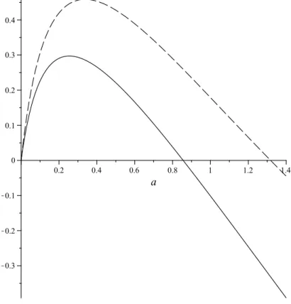
(6) M. BEAU1 , R. BENGURIA2 , R. BRUMMELHUIS3 , P. DUCLOS4. 6. the ground-state energy of the molecule at fixed internuclear distance2. To prove that e(a) is an eigenvalue we have to show, according to the HVZ-theorem, that (1) e(a) is strictly less than the inf of the spectrum of hδ , that is: 1 e(a) < − α0 (a)2 . 2 We can derive a simple variational upper bound for e(a) by using ϕ0 ⊗ ϕ0 as testfunction. Explicit evaluation of Z ® 2 2 ϕ0 (z)4 dz, δ(z1 − z2 ), ϕ0 (z1 )ϕ0 (z2 ) = (11). R. then leads to the upper bound eUB (a, Z) := −α0 (a)2 + Z −1 f (a). (12) where (13). f (a) = α0 ·. 8 cosh4 (aα0 ) + sinh(4aα0 ) + 8 sinh(2aα0 ) + 12aα0 , 4(e2aα0 + 2aα0 + 1)2. which can also be expressed as (14). f (a) = α0 ·. e4aα0 + 4e2aα0 + 4 sinh(2aα0 ) + 12aα0 + 3 . 4(e2aα0 + 2aα0 + 1)2. It is elementary to show that f (a) ≤ 12 α0 (a), the inequality being sharp for a = 0. The simple upper bound (12) suffices to show that the ground state of hδ (a) exists for any a ≥ 0: Proof of theorem 2.1(i). It suffices to show that eUB (a, Z) ≤ − 12 α0 (a)2 for Z ≥ 1. But this follows from eUB (a, Z) ≤ −α0 (a)2 + α0 (a)/2Z ≤ −α0 (a)2 + α0 (a)/2 < −α0 (a)2 /2, since α0 (a) > 1 for a ≥ 0. ¤ To show existence of the molecule, we examine when mina E UB (a) < lim inf a→∞ E(a), where ε (15) E UB (a) := E UB (a, Z, ε) := eUB (a) + , 2a the variational upper bound for the molecule’s energy. We note the trivial lower bound: ε (16) E(a, Z, ε) ≥ E(a, ∞, ε) = −α0 (a)2 + =: E NI (a, ε), 2a where “NI” stands for non-interacting electrons. Clearly, lim inf a→∞ E(a) ≥ lima→∞ E NI (a) = lima→∞ −α0 (a)2 = −1, so to show existence of the molecule it suffices to show that there exists an a ≥ 0 such that E UB (a, Z, ε) < −1, or, equivalently, ε < j(a, Z), where ¡ ¢ (17) j(a, Z) := 2a α0 (a)2 − 1 − Z −1 f (a) . To derive a result which is valid for all Z ≥ 1, we note that Z ≥ 1 implies that j(a, Z) ≥ j(a, 1). The molecule will therefore exist for any value of the parameter ε = Z/L which is less that maxa j(a, 1), for any Z ≥ 1. For the case of Z = 2, we have to have that ε < maxa j(a, 2). Part (ii) of theorem 2.1 is then an immediate consequence of the following lemma: Lemma 3.1. j(a, 1) has a global maximum of 0.297 on a ≥ 0, which is attained for a = 0.254. The maximum of j(a, 2) is equal to 0.458, and is attained for a = 0.337. 2as a notational convention, we denote electronic Hamiltonians and energies by lower case. letters hδ , e(a), eUB (a), etc. and the corresponding molecular entities (obtained by adding ε/2a) by upper case letters Hδ , E(a), E UB (a), etc..

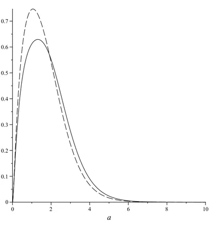
(7) H2 MOLECULE IN STRONG MAGNETIC FIELDS. 7. This lemma has been checked numerically, using Maple: see figure 1 for the graphs of j(a, 1) and j(a, 2).. Figure 1. Graphs of j(a, 1) (—) and j(a, 2) (- - -) Remarks 3.2. (i) Our reliance, here and below, on numerical analysis may be felt to be somewhat unsatisfactory, and it may be possible, with sufficient effort, to give a rigorous analytic proof of lemma 3.1, since j(a, Z) has an explicit analytic expression (and similarly for g(a, Z) below). This lemma of course concerns only one particular variational bound (using a simple test-function) which is unlikely to be optimal, although numerically it does not perform badly (cf. figure 4 below). It would also be interesting to find better variational bounds, if possible again with closed analytic expressions. (ii) The Taylor expansion of j(a, Z) in a = 0 starts of as j(a, Z)/2 = (3 − Z −1 )a + O(a2 ), so that maxa j(a, Z) will be strictly positive if Z > 1/3. Graphical analysis shows that j(a, Z) ≤ 0 when Z = 1/3 and therefore for all Z ≤ 1/3 (note that lima→∞ j(a, Z) = −∞). These remarks imply that the present method would prove existence of the molecule for all Z > 1/3, for sufficiently large L(B), provided we can show that hδ (a, Z) possesses a ground state for such Z, at least for those a for which j(a, Z) > 0. To determine mina E UB (a, Z), we have to solve ∂a eUB = ε/2a2 , or (18). ¡. g(a, Z) = ε,. ¢ where g(a, Z) := 2a + Z −1 f 0 (a) , the prime indicating differentiation. Graphical analysis of g(a, Z) using Maple or Mathematica shows that (18) has two solutions as long as ε < maxa g(a, Z) - see figure 2 below. 2. −2α0 (a)α00 (a).

(8) M. BEAU1 , R. BENGURIA2 , R. BRUMMELHUIS3 , P. DUCLOS4. 8. Figure 2. Graphs of g(a, 1) (—) and g(a, 2) (- - -) It follows (again only graphically, for the time being) that E UB (a, Z, ε) has two critical points, of which the smaller one, for sufficiently small ε, turns out to be a local minimum and the larger a local maximum3. The local minimum is of course a global one under the hypotheses of theorem 2.1(ii). UB Let the minimum of E UB (a, Z, ε) be attained in a = aUB eq (ε); aeq (ε) would be the equilibrium position of the molecule if its energy were in fact equal to our upper bound. It then follows (from the graph of g(a, Z)) that aUB eq (ε) → 0 as ε → 0. This information turns out to be sufficient to determine its small-ε asymptotics, using a simple argument which we will also use in the next section for the true equilibrium position of H2 (δ)-molecule:. Lemma 3.3. As ε → 0, (19). √ aUB eq (ε) ' c ε,. with constant c equal to (20). 1. 1 c= p = UB 0 2 2(e ) (0). r. Z . 8Z − 1. Proof. We fix Z and write eUB (a, Z) = eUB (a). Then aUB eq (ε) is the smallest of the two solutions, a = a− (ε), of (eUB )0 (a) = (2a2 )−1 ε, so that r ε . a− (ε) = UB 0 2(e ) (a− (ε)) 3as follows by further numerical analysis: for example, in the stationary points of E UB (a), we −1 f 00 (a)+a−3 g(a, Z), and the latter function have that (E UB )00 (a) = −2α00 (a)2 −2α0 (a)α00 0 (a)+Z is positive for a in a neighborhood of 0 (e.g. for a < 2 in case Z = 2).

(9) H2 MOLECULE IN STRONG MAGNETIC FIELDS. 9. Now, as we observed above, a− (ε) → 0 as ε → 0, and therefore (eUB )0 (a− (ε)) → (eUB )0 (0), from which the first asymptotic equality of (19) follows. For the second equality, we use that eUB (a) = −(4 − Z −1 ) + (16 − 2Z −1 )a + O(a2 ). ¤ Note that the argument we gave here is very general, and we will seek to apply it in the next section to the true equilibrium position, aeq (ε) of H2 (δ). The equilibrium position aUB eq (ε) we just studied has of course no real physical significance. We will use it, though, in the next section, to obtain a weak a-priori estimate for aeq (ε). To that effect, we note that if we combine (19) with the Taylor expansion of E UB (a, ε) we find: Corollary 3.4. There exists a constant C > 0 such that √ UB (21) Emin (ε) := min E UB (a, ε) ' −4 + Z −1 + C ε, ε → 0. a. UB In particular, Emin (ε) < −1 for Z ≥ 1 and ε sufficiently small .. One can perform a similar analysis for the lower bound, ε E NI (a, ε) = −α0 (a)2 + , 2a and show that the curve E NI (a, ε) has, for fixed and small enough ε, a local minimum and a local maximum, the local minimum again being absolute for sufficiently small ε; the local maximum lies above lima→∞ E NI (a, ε) = −1. If aNI eq (ε) is the lo√ cation of the minimum, then we have again that aNI (ε) ' c ε with a constant c eq which is now equal to c = (2(eNI )0 (0))−1/2 , and √ (22) min E NI (a, ε) ∼ −4 + C ε, a. for a suitable constant C. We finally observe, from the geometry of the graph of E NI (·, ε), that E N I (a) will be strictly increasing on any interval [aNI eq (ε), A] such that E NI (A, ε) < −1 = lima→∞ E NI (a). 4. Asymptotics of aeq (ε) Recall that e(a) := e(a, Z) is the ground-state energy of hδ , and that E(a, ε) = e(a) + ε/2a. As we have seen, E(a, ε) possesses an absolute minimum if ε = Z/L is sufficiently small. It is not a priori known whether this minimum is unique, though we would expect it to be. Below, we let aeq (ε) be any value of a at which E(a, ε) attains its absolute minimum in a on [0, ∞). We will use the following lemma on differentiability of e(a), whose proof we postpone till the the end of this section, in order not to interrupt the flow of the argument. Lemma 4.1. The ground-state energy e(a) is continuously differentiable on [0, ∞). In particular, its right-derivative e0 (0+ ) in 0 exists. Moreover, e0 (0+ ) > 0 for Z > 1/4. The next lemma takes up the idea of lemma 3.3 but now for e(a) directly. Lemma 4.2. Let a = a(ε) be a solution of e0 (a) = ε/2a2 for which there exists a constant A > 0 such that (1) a(ε) ∈ [0, A] for ε sufficiently small; (2) mina∈[0,A] e0 (a) > 0. Then as ε → 0, r ε (23) aeq (ε) ' . 2e0 (0+ ).

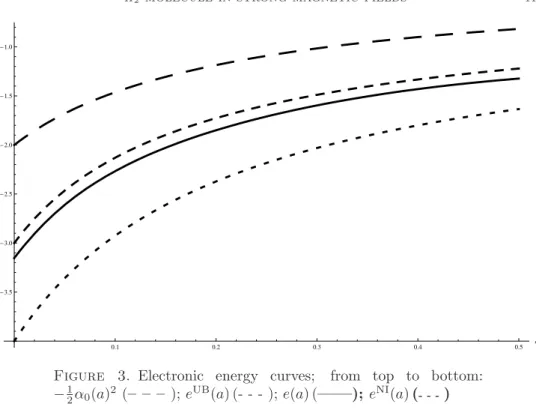
(10) 10. M. BEAU1 , R. BENGURIA2 , R. BRUMMELHUIS3 , P. DUCLOS4. Proof. Since 2a(ε)2 = ε/e0 (a(ε)) ≤ ε/ min[0,A] e0 (a) → 0 as ε → 0, it follows that e0 (a(ε)) → e0 (0+), and hence that 2a(ε)2 /ε → e0 (0+)−1 . ¤ UB We next use E NI (a, ε) and Emin (ε) (cf. lemma 3.4) to effectively bound aeq (ε) (compare [BBDPV1], proof of theorem 2). We assume ε sufficiently small for E UB (ε) < −1 to hold: cf. corollary 3.4. UB (ε) < −1. Let A = Lemma 4.3. Suppose that ε is sufficiently small so that Emin NI UB A+ (ε) be the largest of the two roots of E (A, ε) = Emin (ε). Then aeq (ε) ≤ A+ (ε).. Proof. We first claim that E NI (aeq (ε), ε) < −1. For otherwise, E(aeq (ε), ε) ≥ UM E NI (aeq (ε), ε) ≥ −1 which is in contradiction with E UB (ε) < −1 (since Emin (ε) dominates the ground-state energy of Hδ ). Suppose now that aeq (ε) is strictly larger than A+ (ε) which, as the larger root, is bigger than aNI eq (ε). It then follows from the properties of a → E NI (a, ε) that E NI (a, ε) will be strictly increasing on the NI NI interval [aNI eq (ε), aeq (ε)], and hence E(aeq (ε), ε) ≥ E (aeq (ε), ε) > E (A+ (ε), ε) = UB Emin (ε) ≥ E(aeq (ε), ε), which is a contradiction. ¤ One might hope that the previous lemma, combined with lemma 3.3, would already imply that aeq (ε) → 0, in which case lemma 4.2 together with e0 (0+) > 0 would already imply theorem 2.2. However, √ this is unfortunately not the case: if A+ (ε) → 0, then since A+ (ε) ≥ aUB (ε) ∼ ε, eq √ E NI (A+ (ε), ε) ≤ α0 (A+ (ε))2 + c ε → α0 (0)2 = −4, UB but on the other hand E NI (A+ (ε), ε) = Emin (ε) → −3 + Z −1 , by (21), which is a contradiction. However, it is easy to show that aeq (ε) = O(1) as ε → 0, since if A+ (εν ) → ∞ on some sequence εν → 0, then εν E NI (A+ (εν ), εν ) = −α0 (A+ (εν ))2 + → −1, A+ (εν ) which contradicts √ UB E NI (A+ (εν ), εν ) = Emin (εν ) ' −4 + Z −1 + C εν → −4 + Z −1 ,. as long as Z > 1/3. If we now would know that e0 (a) > 0 for all a ≥ 0, this O(1)estimate for aeq (ε) in combination with lemma 4.2 would prove theorem 2.2. We were however not able to prove monotonicity of e(a). What we can do is give an effective upper bound for aeq (ε), which means we only have to check monotonicity numerically on some known finite interval. UB Lemma 4.4. Let Z ≥ 1 and let ε be such that Emin (ε) ≤ −2: √ (this is true for all sufficiently small ε by Corollary 3.4). Then A+ (ε) ≤ α0−1 ( 2) = 0.3116. Consequently, aeq (ε) ≤ 0.3116.. Proof. Elementary, if we draw the graphs of E N I (a, ε) = −α0 (a)2 + ε/2a, of −α0 (a)2 , which is an increasing function from -4 in 0 to -1 at infinity, and of the UB constant functions Emin (ε) and −2. ¤ √ −1 We can therefore take α0 ( 2) in lemma 4.2 (smaller A’s are also possible, e.g. for Z = 2, depending on how large we are willing to let Z be or how small ε). To finish the proof √ of theorem 2.2 we verify numerically that e(a) is strictly increasing on [0, α0−1 ( 2)]. This can be done using Pierre Duclos’ skeleton method to compute e(a), and has been carried out by one of us in [Be]. The plot of e(a) reveals its monotonicity over the desired interval, thereby completing the proof of theorem 2.2: see figure 3, which for comparison also shows the one-electron energy − 12 α0 (a)2 , as well as eUB (a) and eNI (a). We note in particular, here and also in figure 4 below, that our variational upper bound, though relatively naive, gives a quite reasonable approximation to the actual ground-state energy..

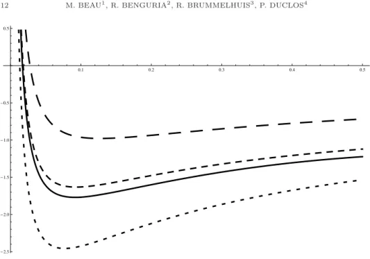
(11) H2 MOLECULE IN STRONG MAGNETIC FIELDS. 11. -1.0. -1.5. -2.0. -2.5. -3.0. -3.5. a 0.1. 0.2. 0.3. 0.4. 0.5. Figure 3. Electronic energy curves; from top to bottom: − 12 α0 (a)2 (– – – ); eUB (a) (- - - ); e(a) (——); eNI (a) (- - - ). The skeleton method allows us to numerically compute the equilibrium distance and energy of the H2 (δ)-molecule for a given Z and L. We discuss by way of example the case of a Hydrogen molecule (Z = 1) in a magnetic field with fieldstrength corresponding to L = 10, or B = L2 eL ' 2.2 106 . We recall (cf. for m 3 e3 c example [BBDP]) that the magnetic field is measured in units of B0 = ~e 3 = 2.35 × 109 G = 2.35 × 105 T , where G stands for Gauss and T for Tesla. Moreover, eB0 the energy is measure in units of ~ω0 = ~ m = 27.2eV = 1 Hartree, where ω0 is the ec 2. cyclotron frequency, and distance in units of the Bohr radius a0 = m~e e2 = 0.53Å. Our L = 10 therefore corresponds to a magnetic field of 5.17 1011 T , which is of course not realizable on earth, but may be realistic for a neutron star. Figure 4 displays the graph E(a) (solid line) as well as, for the sake of comparison, that of E UB (a) (medium dash line), E NI (a) (small dash line) and − 12 α0 (a)2 + ²/2a (large dash line). We see that aeq ≈ 0.1 and Eeq ≈ −1.75, which corresponds to an equilibrium energy of ~ω0 × −1.75 = −47.6eV = −1.75 Hartree and an equilibrium 2a ≈ 10−2 Å. The equilibrium distance is much smaller distance of Req = a0 × LZ than a0 but still significantly bigger than the distance of ≈ 10−5 Å over which the nuclear interaction between two protons makes itself felt. Nevertheless, following [AH3], it may be small enough to significantly enhance the probability for protons to pass through the electronic barrier and be trapped in the nuclear well. It would be interesting to compute the tunnelling cross-section in the Gamov model for the H2 (δ)-model, as simplified model for the actual H2 molecule. We finish with the promised proof of lemma 4.1. Proof of lemma 4.1. We will carry out the proof for the N -electron Hamiltonian ! Ã X X 1 X 1 δ(zi ± a) + (24) hδ (a) := − ∆i − δ(zi − zj ), 2 Z i<j ± i.

(12) 12. M. BEAU1 , R. BENGURIA2 , R. BRUMMELHUIS3 , P. DUCLOS4. 0.5. a 0.1. 0.2. 0.3. 0.4. 0.5. -0.5. -1.0. -1.5. -2.0. -2.5. Figure 4. Molecular energy curves; from top to bottom: − 12 α0 (a)2 + ε/2a (– – – ); E UB (a) (- - - ); E(a) (——); E NI (a) (- - - ). where we will suppose, to fix ideas, that a ≥ 0 (though this is not strictly speaking necessary). Differentiability of e(a) follows from norm-differentiability of the resolvent, which can be established using the symmetrized resolvent equation - we skip the details. We next study e0 (a). Let ψa be the normalized ground-state eigenfunction of hδ (a) on L2 (RN ), which is unique. A formal application of the Feynman-Hellman theorem would lead to e0 (a) = −. XX i. ±. (δ 0 (zi ± a)ψa , ψa ) = −. XX i. hδ 0 (zi ± a), |ψa |2 i.. ±. However, we have to be careful here: since ∂zi ψa a priori has a jump in zi = ±a, |ψa |2 is not an admissible test-function for δ 0 (zi ± a). We will first establish Feynman-Hellman on the level of quadratic forms. If we write ψa (z) = ψ(z, a) (to more clearly bring out the parameter dependence in the notations), the eigen-equation hδ (a)ψa = e(a)ψa translates into XXZ XZ 1 ψ(·, a) ϕ+Z −1 (∇ψ(·, a), ∇ϕ)− ψ(·, a) ϕ = e(a)(ψ(·, a), ϕ), 2 zi =±a ± i i<j zi =zj for all ϕ in H 1 (RN ), the form-domain of hδ (a) We now carefully differentiate with respect to a, taking into account that ψ(·, a) is only left- and right- differentiable with respect to zi in zi = ±a. Furthermore, the derivative of the arbitrary H 1 function ϕ only exists in L2 -sense. However, anticipating that we will take ϕ = ψa = ψ(·, a) below, we assume that the relevant left- and right- derivatives of ϕ also exist. Using the norm-differentiability of ψ(·, a) with respect to a (as an L2 -valued.

(13) H2 MOLECULE IN STRONG MAGNETIC FIELDS. 13. function of a) and taking right-derivatives with respect to a, we arrive at: XX Z 1 (∇∂a ψ(·, a), ∇ϕ) − ∂a ψ(z1 , . . . ± a, . . . , zN , a) ϕ(z1 , . . . , ±a, . . . zN ) 2 RN −1 ± i XZ − ∂zi ψ(z1 , . . . a+ , . . . , zN , a) ϕ(z1 , . . . , a, . . . , zN ) i. RN −1. i. RN −1. i. RN −1. i. RN −1. XZ. −. XZ. +. XZ. +. Z −1. +. ψ(z1 , . . . a, . . . , zN , a) ∂zi ϕ(z1 , . . . , a+ , . . . , zN ) ∂zi ψ(z1 , . . . − a− , . . . , zN , a) ϕ(z1 , . . . , a, . . . , zN ) ψ(z1 , . . . a, . . . , zN , a) ∂zi ϕ(z1 , . . . , −a− , . . . , zN ). XZ. ∂a ψ(·, a) ϕ. zi =zj. i<j. e(a)(∂a ψ(·, a), ϕ) + e0 (a)(ψ(·, a), ϕ).. =. (Note that the right-derivative (with respect to a) of a term such as ψ(z1 , . . . , −a, . . . zN ) is −∂zi ψ(z1 , . . . , −a− , . . . , zN ).) As announced, we now take ϕ = ψ(·, a). Writing again ψa for ψ(·, a) and using real-valuedness of ψa (being the ground state function), we then arrive at the identity XZ 2ψa (z1 , . . . , a, . . . , zN ) ∂zi ψa (z1 , . . . a+ , . . . , zN ) (hδ (a)∂a ψa , ψa ) − + =. i. RN −1. i. RN −1. XZ. 2ψa (z1 , . . . , −a, . . . , zN ) ∂zi ψa (z1 , . . . − a− , . . . , zN ). e(a)(∂a ψa , ψa ) + e0 (a)(ψa , ψa ).. Since (hδ (a)∂a ψa , ψa ) = (∂a ψa , hδ (a)ψa ) = e(a)(∂a ψa , ψa ), we have proved: Lemma 4.5. (Feynman-Hellman for hδ (a)). Let ψa be the normalized ground-state of h(a). Then ¶ Z Z Xµ 0 (25) e (a) = −2 ψa ∂zi ψa + 2 ψa ∂zi ψa . zi =a+. i. zi =−a−. End of the proof of lemma 4.1. If we now let a → 0 in (25), and use the boundary conditions at a = 0 for membership of the domain of hδ (0), we obtain that XZ e0 (0+ ) = 2 (∂zi ψ0 |zi =0− − ∂zi |zi =0+ ) ψ0 = Since, finally, XZ 2 i. zi =0. ψ02. 4. i. zi =0. i. zi =0. XZ. ψ02 ≥ 0.. =. X 1 ||∇ψ0 ||2 + (δ(zi − zj )ψ0 , ψ0 ) − ( hδ (0) ψ0 , ψ0 ) 2 i<j. ≥. −( hδ (0) ψ0 , ψ0 ) = −e(0),. we find, specializing to N = 2 again, that e0 (0+ ) ≥ −2e(0) ≥ −2eUB (0) = 2α0 (0)2 − 2Z −1 f (0) = 2α0 (0)2 − Z −1 α0 (0) > 0 as long as Z > (2α0 (0))−1 = 1/4. ¤.

(14) 14. M. BEAU1 , R. BENGURIA2 , R. BRUMMELHUIS3 , P. DUCLOS4. 5. Conclusions We have approximated the H2 -molecule in a constant magnetic field, as described by the non-relativistic Pauli Hamiltonian with fixed nuclei, by a two-electron modelHamiltonian of a one-dimensional molecule with electron-electron and electronnuclei interaction given by δ-potentials, and interaction between the two nuclei given by the usual Coulomb potential. It can be shown, using the methods of [BD3], that this approximation is exact in the large field limit. We have shown, for this approximation, that the ground state of the molecule exists, for any nuclear charge Z ≥ 1 and for sufficiently large magnetic fields, and that the (re-scaled) internuclear equilibrium distance of the molecule tends to 0 with increasing field-strength B, at a rate of (log B)−1/2 . This generalises earlier results for H2+ in [BBDP], [BBDPV1], [BBDPV2]. Of the numerous questions which remain, the foremost one is to extend these results to the full Pauli-Hamiltonian. This was possible for the single-electron H2+ -ion, but the argument for the equilibrium distance given in [BBDPV1] used the exact solution of the δ-model. In the case of the two-electron H2 such exact solutions are not available anymore, despite the apparent simplicity of the δ-potentials, and we have had in part to rely on numerical computations to prove our results, notably to establish monotonicity of the electronic ground-state energy as function of the inter-nuclear distance. Since this would already imply that the inter-nuclear distance tends to 0 at the proper rate (cf. the remarks just before lemma 4.4), it would be very interesting to find an analytical proof of this monotonicity, or at least on a sufficiently large interval (such as the one specified in lemma 4.4). Another interesting question which remains open is that of uniqueness of the equilibrium position, for the δ-approximation as well as for the full Paulimolecule. We also relied on numerical computations in the study of our variational upper bound and lower bounds. Here it may be possible to give analytic proofs, since these upper and lower bounds have analytically closed expressions involving a particular and well-understood special function, the Lambert W -function. It would furthermore be interesting to find sharper variational upper bounds, e.g. by using test functions which incorporate electron-electron correlations. Other perspectives are to go beyond the Born–Oppenheimer approximation and analyse the effect of nuclear vibrations on the stability of the nuclei, and to compute the probability of tunnelling through the Coulomb barrier. Finally, it would be interesting to see to what extend the methods and results of this paper can be extended to diatomic molecules with an arbitrary number of electrons. Some (unpublished) work in this direction was already started by Pierre Duclos.. References 2+ J. Ackermann, H. Hogreve: On the metastability of the 1 Σ+ and g ground state of He2 2+ N e2 : a case study of binding metamorphosis, J. Phys. B: At. Mol. Opt. Phys. 25, 4069 (1992). [AH2] J. Ackermann, H. Hogreve: Comment on: ”Accurate adiabatic potentials of the two 2+ lowest 1 Σ+ g states of He2 , J. Phys. B: At. Mol. Opt. Phys. 32, 5411 (1999). [AH3] J. Ackermann and H. Hogreve: The magnetic two-centre problem: Nuclear fusion catalyzed by ultrastrong fields?, Few-Body Systems 41 (3-4), 221 - 231 (2007). [AtMol] Atoms and Molecules in Strong External Fields, P. Schmelcher and W. Schweizer (Eds.), Plenum Press, N.Y. (1998), Springer (2002). [AM] C. Amovilli, N. March: Feynmann propagator and Slater sum for a model Hamiltonian motivated by H2+ in an intense magnetic field, Int. J. Quantum Chem. 106, 533 - 541 (2005). [BaSoY] B. Baumgartner, J.-Ph. Solovej, J. Yngvason: Atoms in strong magnetic fields: The high field limit at fixed nuclear charge, Commun. Math. Physics 212 (3), 703 - 724 (2000).. [AH1].

(15) H2 MOLECULE IN STRONG MAGNETIC FIELDS. 15. [Be]. M. Beau: Sur la fusion de deux noyaux par un champ magnétique intense, Projet Master 2ième année, CPT Marseille (2007). [BD1] R. Brummelhuis, P. Duclos: On the one dimensional behaviour of atoms in intense homogeneous magnetic fields, Proceedings of the PDE2000 conference in Clausthal, Germany: Partial Differential Equations and Spectral Theory. M. Demuth, B.-W Schulze eds. Operator Theory, Advances and Applications 126, pp 25-35, Birkhäuser Verlag Basel (2001). [BD2] R. Brummelhuis, P. Duclos: Effective Hamiltonians for atoms in very strong magnetic fields, Few-Body Systems 31, 1-6 (2002). [BD3] R. Brummelhuis, P. Duclos: Norm-resolvant convergence to effective Hamiltonians for atoms in very strong magnetic fields, J. Math. Phys. 47, 032103 (2006). [BBDP] R. Benguria, R. Brummelhuis, P. Duclos, S. Pérez-Oyarzún, H2+ in a strong magnetic field, J. Physics B: At. Mol. Opt. Phys. 36 (11), 2311-2320 (2004). [BBDPV1] R. Benguria, R. Brummelhuis, P. Duclos, S. Pérez-Oyarzún, P. Vytřas, Equilibrium nuclear separation for the H2+ molecule in a strong magnetic field, J. Phys. A: Math. Gen. 39, 8451-8459 (2006). [BBDPV2] R. Benguria, R. Brummelhuis, P. Duclos, S. Pérez-Oyarzún, P. Vytřas, Non-relativistic H2+ -molecule in a strong magnetic field, Few-Body Systems 38 (2-4), 133 - 137 (2006). [BBDR] D. Bressanini, R. Brummelhuis, P. Duclos, R. Ruamps, Can one bind three electrons with a single proton?, Few-Body Systems 45 (2-4), 173 - 177 (2009). [CGHJK] R.M. Corless, G.H. Gonnet, D.E. Hare, D.J. Jeffrey, D.E. Knuth, On the lambert W function, Adv. Comp. Math. 5, 329 (1996) [CDR] H. D. Cornean, P. Duclos and B. Ricaud, On critical stability of three quantum charges interacting through delta potentials, Few-Body Systems 38 (2-4), 125 - 131 (2006). [DSC] T. Detmer, P. Schmelcher, L. S. Cederbaum: Hydrogen molecule in a magnetic field: The lowest states of the Π manifold and the global ground state of the parallel configuration, Phys. Rev. A 57, 1767 (1998). [DSDC] T. Detmer, P. Schmelcher, F. K. Diakonos, L. S. Cederbaum: Hydrogen molecule in magnetic fields: The ground states of the Σ manifold of the parallel configuration, Phys. Rev. A 56, 1825 (1997). [RFGS] J. M. Richard, J. Fröhlich, G.-M. Graf, M. Seifert: Proof of stability of the hydrogen molecule, Phys. Rev. Lett. 171, 1332 (1993). [Ho] H. Hogreve: The δ point interaction two center system, Int. J. Quantum Chem. 109, 1430 - 1441 (2009). [La] D. Lai: Matter in strong magnetic fields, Rev. Mod. Phys. 73, 629 - 662 (2001). [L] E. H. Lieb: Monotonicity of the molecular electronic energy in the nuclear coordinates, J. Phys. B: At. Mol. Phys. 11 (3) (1982). [LS] E. H. Lieb, B. Simon: Monotonicity of the electronic contribution to the BornOppenheimer energy, J. Phys. B: At. Mol. Physics 11 (18) (1978). [LSY] E. H. Lieb, J.-Ph. Solovej, J. Yngvason: Asymptotics of heavy atoms in high magnetic fields: I. lowest Landau band regions, Commun. Pure Appl. Math. 52, 513 - 591 (1994). [NeuSt] Isolated Neutron Stars: from the Interior to the Surface, S. Zane, R. Turolla and D. Page (Eds.), Springer (2007). [Ros] C.M. Rosenthal: Solution of Delta Function Model for Heliumlike Ions, Journ. Chem. Phys. 35(5), 2474-2483 (1971). [Tu] A. Turbiner: A. Turbiner: Molecular systems in a strong magnetic field, pp. 267 - 277 in [NeuSt]. [TG] A. V. Turbiner, N. L. Guevara: He2+ molecular ion can exist in a magnetic field, Phys. 2 Rev. A 74, 063419 (2006). 1,4 Centre de Physique Théorique UMR 6207 - Unité Mixte de Recherche du CNRS et des Universités Aix-Marseille I, Aix-Marseille II et de l’ Université du Sud ToulonVar - Laboratoire affilié à la FRUMAM, Luminy Case 907, F-13288 Marseille Cedex 9 France. 2. Departamento de Fı́sica, P. Universidad Católica de Chile, Santiago, Chile.. 3 Department of Economics, Mathematics and Statistics, Birkbeck, University of London, Malet Street, WC1E 7HX London, United Kingdom and Laboratoire de Mathématiques de Reims, EA 4535..

(16)