HATS 43b, HATS 44b, HATS 45b, and HATS 46b: Four Short period Transiting Giant Planets in the Neptune Jupiter Mass Range
23
0
0
Texto completo
(2) 2. Brahm et al. 1. INTRODUCTION. By measuring their masses and radii, transiting planets orbiting moderately bright stars offer the unique opportunity of studying in depth the physical structure of planets other than those present in the solar system. This property makes transiting planets one of the most valuable resources for testing current models of planet formation and evolution (e.g., Mordasini et al. 2012). In addition, detailed follow-up observations of these systems allowed us to study the structure and composition of their atmospheres (e.g., Fraine et al. 2014), and to refine their orbital configuration and evolution by measuring the misalignment angle between the orbit and the spin axis of their host stars (e.g., Zhou et al. 2015). Ground-based photometric surveys like HATNet (Bakos et al. 2004) and SuperWASP (Pollacco et al. 2006) have been a key and cost-efficient resource in contributing to the current number of ∼300 discovered transiting systems with masses and radii determined with a precision better than 30%. Even though the population of discovered systems is highly biased towards the detection of giant planets at short distances from their stars (hot Jupiters), the increase of discoveries in this narrow region of the parameter space has proven to be fundamental for achieving statistically significant results that are helping to solve some of the theoretical challenges present in the field. For example, Hartman et al. (2016), using the full population of well characterised transiting systems, found that the radii of close-in planets increase as the parent stars evolve. This fact supports the theories that propose that hot Jupiters are inflated due to energy deposited deep into the planet interior (e.g. Batygin & Stevenson 2010) and not due to a delayed cooling (Burrows et al. 2007). Another recent example concerning the using of the full population of well characterised transiting systems is that of Hellier et al. (2017), who find that there is no difference within the so-called Jupiter bulge between the planetary period distributions around greater-than versus less-than-solar metallicity host stars. This calls into question the idea that the lack of hot Jupiters discovered by the Kepler mission is due to a bias in the metallicity of the Kepler sample (Dawson & Murray-Clay 2013). Despite the importance of continuing the discovery of short period gas giants, most of the efforts of the community are being put into the detection of well characterised transiting planets located in sparsely populated regions of the parameter space. Planets with periods longer than ten days and/or sub-Saturn mass planets are particularly interesting. While these types of planets are among the prime discovery targets of the ongoing Kepler K2 mission (Howell et al. 2014), and will be also efficiently discovered by TESS (Ricker et al. 2014), several new ground-based photometric surveys were designed to dig into these planetary regimes. Specifically, the HATSouth survey of robotic telescopes (Bakos et al. 2013), having three stations in three well separated locations in the southern hemisphere, has an increased efficiency for detecting both longer period giant planets (warm Jupiters), and planets with in the Neptune-Saturn mass range, if compared to typical single site surveys. The ability of the HATSouth network to discover these type of systems has been already demonstrated with the discoveries of two. super-Neptunes (Bakos et al. 2015; Bayliss et al. 2015), and of a warm Jupiter with an orbital period of ≈ 16 days (Brahm et al. 2016). In this paper we present the discovery of four new well characterised short-period transiting planets from the HATSouth survey. In Section 2 we summarise the detection of the photometric planetary signal, and spectroscopic and photometric follow up observations. In Section 3 we describe the analysis that was carried out in order to rule out false positives, and to derive the parameters of the planets and host stars. Finally, in Section 4 we summarise the properties of each system and we discuss our findings in the context of the full population of discovered transiting systems. 2. OBSERVATIONS 2.1. Photometric detection The discovery of the periodic planetary-like photometric signals for the four systems presented in this study were obtained from the images registered by the three stations of the HATSouth network (the HS1 and HS2 instruments in Chile, HS3 and HS4 in Namibia, and HS5 and HS6 in Australia). Observations were performed with a typical cadence of 5 minutes using a Sloan r photometric filter. The specific properties of the observations that allowed the discovery of the planets are summarised in Table 1. As can be noticed in this table, the total number of images obtained per station varies from 700 to 9000 images, and were strongly dependent on the weather conditions and technical issues present on each site. In addition, the number of images obtained for different objects also depends on the adopted observing strategy and the position of the target in the field, because targets located in the edges of fields are usually also monitored when observing contiguous fields, as is the case in this work for HATS-44 and HATS-46. The original images were reduced to photometric light curves by following the procedures described in Penev et al. (2013). The light curves thus generated were corrected for systematic signals using the Trend Filtering Algorithm (TFA, Kovács et al. 2005) and then the Box Least Squares (BLS, Kovács et al. 2002) method was applied to identify periodic transit-like features on them. Figure 1 shows the phase-folded light curves for the four systems analysed in this study, which presented periodic dimmings in their fluxes with depths (10–30 mmag) and durations (1.6–3.2 h) compatible with being short-period transiting giant planets. Due to these properties, these systems were added to the HATSouth database of planetary candidates. The light curve data for these four systems are presented in Table 3. 2.2. Spectroscopic Observations. To confirm the planetary nature of the candidates discovered by the HATSouth network, they are subject of an extensive follow-up campaign that involves the use of different facilities containing spectroscopic instruments with a wide range of capabilities. All the spectrographs used for the discovery of the four HATS planets presented in this work are listed in Table 2 along with the general properties of the observations. 2.2.1. Reconnaissance Spectroscopy.
(3) HATS-43b–HATS-46b. 3. HATS-43. HATS-44. -0.04. ∆ mag. ∆ mag. -0.02 0 0.02 0.04 0.06 -0.4. -0.2. 0. 0.2. -0.04 -0.03 -0.02 -0.01 0 0.01 0.02 0.03 0.04 0.05. 0.4. -0.4. -0.2. 0. Orbital phase. 0.2. 0.4. 0.02. 0.04. 0.2. 0.4. Orbital phase -0.04. -0.04. -0.03 -0.02. ∆ mag. ∆ mag. -0.02 0 0.02. -0.01 0 0.01 0.02 0.03. 0.04. 0.04. 0.06. 0.05 -0.06. -0.04. -0.02. 0. 0.02. 0.04. 0.06. -0.04. -0.02. 0. Orbital phase. Orbital phase. HATS-45. HATS-46. -0.03 -0.01. ∆ mag. ∆ mag. -0.02 0 0.01 0.02 0.03 0.04 -0.4. -0.2. 0. 0.2. -0.04 -0.03 -0.02 -0.01 0 0.01 0.02 0.03 0.04. 0.4. -0.4. -0.2. 0. Orbital phase. -0.03. -0.04. -0.02. -0.03. -0.01. -0.02. ∆ mag. ∆ mag. Orbital phase. 0 0.01 0.02. -0.01 0 0.01 0.02. 0.03. 0.03. 0.04 -0.04. -0.02. 0. 0.02. 0.04. Orbital phase. 0.04 -0.04. -0.03. -0.02. -0.01. 0. 0.01. 0.02. 0.03. 0.04. Orbital phase. Figure 1. Phase-folded unbinned HATSouth light curves for HATS-43 (upper left), HATS-44 (upper right), HATS-45 (lower left) and HATS-46 (lower right). In each case we show two panels. The top panel shows the full light curve, while the bottom panel shows the light curve zoomed-in on the transit. The solid lines show the model fits to the light curves. The dark filled circles in the bottom panels show the light curves binned in phase with a bin size of 0.002.. After the initial photometric detection, the four candidates presented in the previous section were first observed with the WiFeS spectrograph (Dopita et al. 2007) installed at the ANU 2.3m telescope. As described in Bayliss et al. (2013), observations are performed with two instrument configurations. A single R=3000 spectra is obtained for each candidate in order to perform a spectral classification of the star by determining its effective temperature (Teff ), surface gravity (log g) and metallicity ([Fe/H]) by using a library of synthetic spectra with the principal goal of identifying giant stars for which the observed transit depth could not be produced by planetary companions. In this way, HATS-43 and HATS-44 were identified as a K-dwarfs with Teff = 4900 ± 300 K, log g= 5.0 ± 0.3 dex, and Teff = 4750 ± 300 K, log g= 4.3 ± 0.3 dex, respectively, while HATS-45 and HATS46 were typed as a F-dwarf (6250 ± 300 K, 3.7 ± 0.3) and a G-dwarf (5800 ± 300 K, 4.5 ± 0.3), respectively. Additionally multiple spectra for each candidate are obtained with a resolving power of R=7000, with the goal of measuring radial velocity (RV) variations with a precision of ∼2 km s−1 for identifying systems in which the transit-like signal is produced by stellar mass companions. The number of velocity points obtained for each candidate were 2, 4, 3 and 3 for HATS-43 -44 -45 and -46, respectively and they were focused on phases ∼0.25 and ∼0.75 where the maximum velocity difference is expected. No significant velocity variations at the level of ∼4 km s−1 were observed for any of the four candidates. The lack of high-amplitude velocity variations and the. dwarf status of the host stars for the four HATS candidates provided the first evidences in favour of the planetary origin of the photometric signals described in Section 2.1 2.2.2. Precision Radial Velocities. Precision radial velocities are required to confirm the planetary nature of a transiting companion by providing the means to estimate its mass and orbital parameters. For this purpose, we used the FEROS spectrograph (Kaufer & Pasquini 1998) installed at the MPG 2.2m telescope. The high efficiency of this instrument coupled to its high resolving power of R=50000 allows us to achieve a long term radial velocity precision in the range of 10 – 50 m s−1 for our V>13 candidates by obtaining spectra with ∼1800s of exposure time using the simultaneous wavelength calibration technique (Baranne et al. 1996). In the case of HATS-43, -44, and -45, we obtained on the order of 15 FEROS spectra, while for HATS-46, 31 FEROS spectra were acquired. All FEROS spectra were reduced, extracted and analysed using the CERES pipeline (Brahm et al. 2017a), where after applying an optimal extraction algorithm, each spectrum is wavelength calibrated and corrected by instrumental drifts before calculating the radial velocity by cross-correlation with a G2-like binary mask. Bisector spans are also measured for each spectrum by CERES. Figure 3 shows that the FEROS velocities obtained for the four systems have a time correlated variation, which is in phase with the photometric ephemerides and has an amplitude consistent with planetary-mass objects. However, only in the.
(4) 4. Brahm et al. Table 1 Summary of photometric observations Instrument/Fielda. Date(s). # Images. Cadenceb (sec). Filter. Precisionc (mmag). HATS-43 HS-2.4/G598 HS-4.4/G598 HS-6.4/G598 LCOGT 1 m+CTIO/SBIG LCOGT 1 m+CTIO/sinistro. 2013 2013 2013 2016 2016. Sep–2014 Mar Sep–2014 Feb Sep–2014 Mar Aug 21 Oct 26. 739 4154 3865 44 69. 285 345 357 219 219. r r r i i. 13.4 11.4 10.9 1.3 1.1. HATS-44 HS-2.3/G598 HS-4.3/G598 HS-6.3/G598 HS-1.2/G599 HS-3.2/G599 HS-5.2/G599 LCOGT 1 m+SAAO/SBIG LCOGT 1 m+CTIO/sinistro LCOGT 1 m+CTIO/SBIG. 2013 2013 2013 2012 2012 2012 2015 2015 2015. Sep–2014 Sep–2014 Sep–2014 Jan–2013 Jan–2013 Jan–2013 Nov 07 Nov 15 Nov 26. Mar Feb Mar Apr Apr Apr. 745 4143 3836 9325 3174 5004 63 55 41. 285 345 357 292 288 288 194 219 194. r r r r r r i i g. 12.4 13.5 13.3 12.1 12.9 12.7 2.2 5.4 6.9. HATS-45 HS-2.2/G554 HS-4.2/G554 HS-6.2/G554 Swope 1 m/e2v CTIO 0.9 m LCOGT 1 m+SAAO/SBIG LCOGT 1 m+CTIO/sinistro. 2009 2009 2010 2014 2014 2015 2015. Dec–2011 May Dec–2011 Mar Dec–2011 May Mar 22 Oct 13 Mar 09 Mar 14. 6414 953 2097 81 36 25 51. 296 383 300 160 181 200 226. r r r i i i i. 8.0 10.2 8.5 1.6 1.9 1.4 1.5. HATS-46 HS-2.3/G754 HS-4.3/G754 HS-6.3/G754 HS-1.2/G755 HS-3.2/G755 HS-5.2/G755 Swope 1 m/e2v LCOGT 1 m+CTIO/sinistro. 2012 2012 2012 2011 2011 2011 2014 2016. Sep–2012 Dec Sep–2013 Jan Sep–2012 Dec Jul–2012 Oct Jul–2012 Oct Jul–2012 Oct Nov 30 Aug 31. 3875 3191 2994 5265 4851 6018 64 55. 282 292 285 292 287 296 169 219. r r r r r r i i. 9.2 9.9 9.7 9.6 10.3 9.3 1.7 1.1. a. For HATSouth data we list the HATSouth unit, CCD and field name from which the observations are taken. HS-1 and -2 are located at Las Campanas Observatory in Chile, HS-3 and -4 are located at the H.E.S.S. site in Namibia, and HS-5 and -6 are located at Siding Spring Observatory in Australia. Each unit has 4 ccds. Each field corresponds to one of 838 fixed pointings used to cover the full 4π celestial sphere. All data from a given HATSouth field and CCD number are reduced together, while detrending through External Parameter Decorrelation (EPD) is done independently for each unique unit+CCD+field combination. b The median time between consecutive images rounded to the nearest second. Due to factors such as weather, the day–night cycle, guiding and focus corrections the cadence is only approximately uniform over short timescales. c The RMS of the residuals from the best-fit model.. case of HATS-44, the FEROS velocities were enough for measuring the semi-amplitude with a precision better than 25% (K=90±17 m s−1 ). For the remaining candidates additional observations were required as we now describe. HATS-43 and HATS-45 were observed with the HARPS instrument (Mayor et al. 2003) mounted on the ESO 3.6m telescope, which is located at the ESO La Silla Observatory. Observations were performed with the Object+Sky mode because the daily internal drifts of the instrument are smaller than 1 ms−1 which is significantly smaller than the radial velocity precision that we require. HARPS data was also reduced and analysed with CERES. By using these additional velocities, the semi-amplitudes of the orbits for HATS-43 and HATS45 were determined with a precision better than 25%. While the combined RVs for HATS-45 suggest that the star is orbited by a typical hot-Jupiter, the velocities for HATS-43 are consistent with the presence of a Saturnmass planet with a non-negligible eccentricity. For these. two planets we also obtained a single spectrum using the Coralie Spectrograph mounted on the 1.2m Euler telescope installed at the ESO La Silla Observatory. Both spectra were processed with CERES but were not used in the analysis because no velocity variations could be computed from a single radial velocity epoch. Finally, HATS-46 was observed with the Planet Finder Spectrograph (PFS, Crane et al. 2010) mounted on the Magellan/Clay 6.5m telescope at Las Campanas Observatory. As has been described in previous HATSouth discoveries (Jordán et al. 2014; Zhou et al. 2014; Hartman et al. 2015), we obtained a template spectrum by using the 0.500 slit, which was then used as reference for computing the radial velocities at different epochs by obtaining spectra with a I2-cell. The 11 spectra that were acquired with the I2-cell were processed as described in Butler et al. (1996). The mean RV precision achieved was ∼20 ms−1 and was principally limited by the faintness of the star. By combining the velocities measured by FEROS and PFS for HATS-46 we were able to con-.
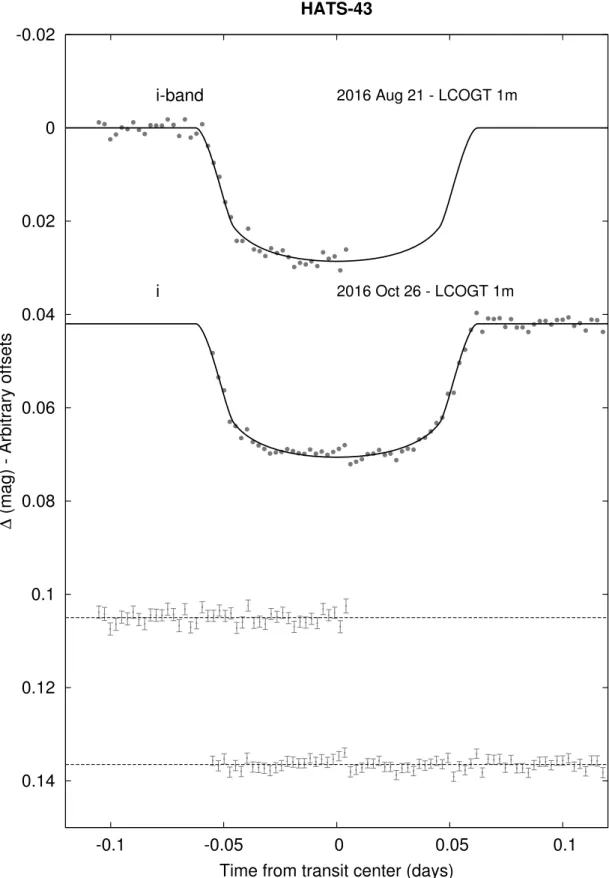
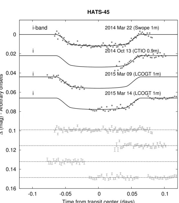
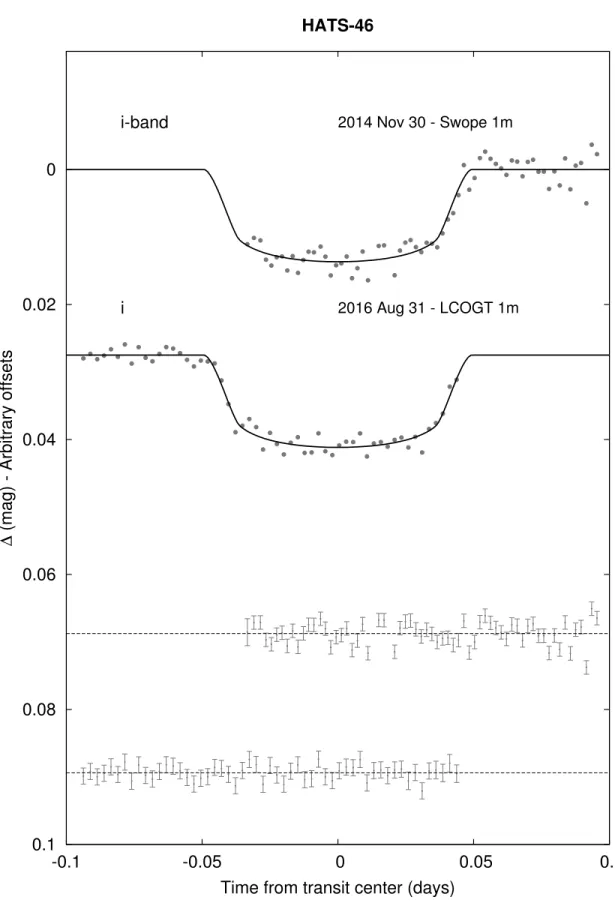
(5) HATS-43b–HATS-46b firm the planetary nature of this candidate and infer for it a sub-Saturn mass. The radial velocities and bisector spans obtained with FEROS, Coralie, and HARPS for the four discovered planets are presented in Table 7 at the end of the paper. We investigated if there is a significant degree of correlation between the radial velocities and the bisector span measurements that could suggest that the observed velocity variations are produced by a blended stellar companion. Specifically, we followed the procedure adopted in Bhatti et al. (2016) and for each of our four systems we computed the error weighted distribution for the Pearson correlation coefficient by applying a bootstrap method. The derived 95% confidence intervals for the correlation coefficient are [-0.57, 0.30], [-0.59, 0.02], [-0.35, 0.46], and [-0.22, 0.65], for HATS-43, HATS-44, HATS-45, and HATS-46, respectively, implying that there is no significant correlation and thus supporting the planetary hypothesis as the cause of the observed velocity variations. Figure 2 shows the radial velocities vs. bisector spans diagrams for each of the four systems. 2.3. Photometric follow-up observations In addition to the HATSouth discovery light curves, we observed transits for the four discovered planets using telescopes with larger apertures in order to: i) confirm that the photometric signals are real, ii) refine the ephemerides of the systems, and iii) measure the transiting parameters with a higher precision; an accurate determination of RP /R? and a/R? is particularly important for obtaining a reliable estimation of the planetary physical parameters. The basic configurations used in these observations are listed in Table 1, while the light curve data is presented in Table 3. As shown in Figure 4, an ingress and an almost full transit including a complete egress of HATS-43b were observed using the 1 m telescope of of the Las Cumbres Observatory Global Telescope (LCOGT) network (Brown et al. 2013) located at the Cerro Tololo International Observatory (CTIO). Both observations were performed during the second semester of 2016, approximately 3 years after the original HATSouth photometry was obtained. Even though both light curves were obtained with the Sloan i band, the one containing the egress was registered by a SBIG camera, while the full transit was registered using the Sinistro camera. In both cases the per-point photometric precision was of ∼1.5 mmag with a cadence of ≈ 219 sec. Three full transits of HATS-44b were observed in November 2015 using the LCOGT 1m network (see Figure 5). The first one was obtained from the South African Astronomical Observatory (SAAO) using the Sloan i filter and a SBIG camera, achieving a photometric precision of ≈ 2 mmag with a cadence of ≈ 200 sec. The second transit was observed from CTIO with the same filter but using a Sinistro camera. The observing conditions were not optimal which resulted in the photometric precision being only ∼5 mmag with a cadence of ≈ 200 sec. The last transit was also observed from CTIO but this time the Sloan g band was used with the goal of checking that there was no colour dependence of the transit depth such as would be produced by a blended eclipsing binary system, given the slightly triangular shape of this transit. Even though the precision obtained for this transit was. 5. relatively low (∼7 mmag with a cadence of ≈ 200 sec), it was enough to confirm that there was no significant variation in the transit depth between the r and g filters. For HATS-45b we obtained four i-band follow-up light curves, which are shown in Figure 6. The first light curve was obtained in March 2014 and registered a full transit using the 1m Swope telescope and e2v CCD camera. The second light curve was obtained on October 2014 using the 0.9m Telescope of CTIO and registered only an egress. The last two light curves were obtained on March 2015 with the LCOGT 1m network, with an ingress observed from SAAO and an egress from CTIO. The photometric precision for these four light curves was in the 1 – 2 mmag range with cadences ≈ 200 sec. Finally, two i-band transits were observed for HATS46b, which are shown in Figure 7. In November 2014 a partial transit containing an egress was observed with the Swope 1m telescope, while in August 2016 we registered a full transit with the LCOGT 1m telescope installed at CTIO using a Sinistro camera. Both light curves achieved a photometric precision below 2 mmag at ≈ 200 sec cadence. The instrument specifications, observing strategies and reduction procedures that we apply in the case of the three instruments that were used to obtain photometry for our four planets have been previously discussed in Bayliss et al. (2015), Penev et al. (2013), and Hartman et al. (2015), for LCOGT, Swope 1m, and CTIO 0.9m, respectively..
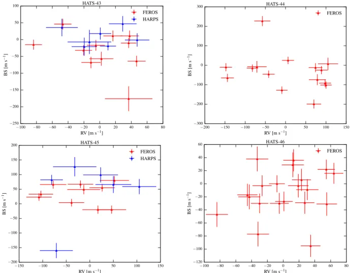
(6) 6. Brahm et al.. HATS-43. 100. HATS-44. 300. FEROS HARPS. 50. FEROS 200. 0. −50. BS [m s−1]. BS [m s−1]. 100. −100. −100. −150. −200. −200 −250 −100. 0. −80. −60. −40. 0. −20. 20. 40. 60. −300 −200. 80. RV [m s−1]. HATS-45. 200. −150. −100. 50. 100. 150. RV [m s−1]. HATS-46. 60. FEROS. FEROS HARPS. 150. 0. −50. 40 20. 100. 0. BS [m s−1]. BS [m s−1]. 50 0. −50. −40 −60. −100. −80. −150 −200 −150. −20. −100 −100. −50. 0. RV [m. 50. s−1]. 100. 150. −120 −100. −80. −60. −40. −20. 0. 20. 40. 60. 80. RV [m s−1]. Figure 2. RV vs bisector span measurements for HATS-43 (upper left), HATS-44 (upper right), HATS-45 (lower left) and HATS-46 (lower right). No significant correlation at the 95% level was identified, which indicates that the RV variations are probably produces by planetary mass orbital companions..
(7) HATS-43b–HATS-46b. 7. Table 2 Summary of spectroscopy observations # Spec.. Res. ∆λ/λ/1000. S/N Rangea. γRV b (km s−1 ). RV Precisionc (m s−1 ). 1 2 12 7 1. 3 7 48 115 60. 68 57–82 15–50 10–24 12. ··· 23.2 22.078 22.053 22.002. ··· 4000 25 24 ···. 2015 Jan 1 2015 Jan–Aug 2015 Oct–2016 Dec. 1 4 15. 3 7 48. 54 50–101 19–36. ··· 47.4 44.082. ··· 4000 50. 2013 2014 2014 2015 2015. Sep 27 Feb 17–23 Sep 12 Jan–2016 Feb Feb 14–19. 1 3 1 13 6. 3 7 60 48 115. 87 44–70 12 22–70 14–24. ··· 20.8 19.19 19.423 19.372. ··· 4000 ··· 50 28. 2014 2014 2015 2015 2015. Oct 4 Oct 4–7 Jun–2016 Dec Jun–2016 Dec Jun. 1 3 31 11 3. 3 7 48 76 76. 64 36–80 16–57 45–55 59–61. ··· -30.5 -30.193 ··· ···. ··· 4000 35 24 ···. Instrument. UT Date(s). HATS-43 ANU 2.3 m/WiFeS ANU 2.3 m/WiFeS MPG 2.2 m/FEROS ESO 3.6 m/HARPS Euler 1.2 m/Coralie d. 2015 2015 2015 2016 2016. Feb 6 Feb 6–8 Oct–2016 Dec Apr–Nov Aug 10. d. HATS-44 ANU 2.3 m/WiFeS ANU 2.3 m/WiFeS MPG 2.2 m/FEROS HATS-45 ANU 2.3 m/WiFeS ANU 2.3 m/WiFeS Euler 1.2 m/Coralie d MPG 2.2 m/FEROS d ESO 3.6 m/HARPS HATS-46 ANU 2.3 m/WiFeS ANU 2.3 m/WiFeS MPG 2.2 m/FEROS d Magellan 6.5 m/PFS+I2 Magellan 6.5 m/PFS a. S/N per resolution element near 5180 Å.. b For high-precision RV observations included in the orbit determination this is the zero-point RV from the best-fit orbit. For other instruments it. is the mean value. We do not provide this quantity for the lower resolution WiFeS observations which were only used to measure stellar atmospheric parameters. c For high-precision RV observations included in the orbit determination this is the scatter in the RV residuals from the best-fit orbit (which may include astrophysical jitter), for other instruments this is either an estimate of the precision (not including jitter), or the measured standard deviation. We do not provide this quantity for low-resolution observations from the ANU 2.3 m/WiFeS. d We excluded from the analysis the single Coralie observations of HATS-43 and HATS-45. We also excluded from the analysis one FEROS observation of HATS-43 obtained on UT 2015 Oct 30, and one FEROS observation of HATS-45 obtained on UT 2015 Feb 2, both of which were affected by significant sky contamination. For HATS-46, which has a very low amplitude RV orbital wobble, and for which even slight sky contamination can obscure the signal, we excluded 11 FEROS observations due to evidence of sky contamination as seen in the computed CCFs. The excluded observations are from UT 2015 Jun 10, and 21, Jul 20, Oct 2, 4, 26, 27 and 30, and Nov 3, and 2016 Jul 26 and Sep 14..
(8) 8. Brahm et al.. HATS-43. HATS-44. FEROS 100 HARPS. FEROS 200. RV (ms-1). 100. 0. 0. -100. -100. -200. 60 40 20 0 -20 -40 -60 -80 -100 100 50 0 -50 -100 -150 -200 -250. 150 100 50 0 -50 -100 -150 -200 300 250 200 150 100 50 0 -50 -100 -150 -200 -250. O-C (ms-1). -50. BS (ms-1). BS (ms-1). O-C (ms-1). RV (ms-1). 50. 0.0. 0.2. 0.4 0.6 Phase with respect to Tc. 0.8. 1.0. 0.0. 0.2. HATS-45. 0.4 0.6 Phase with respect to Tc. 0.8. 1.0. 0.8. 1.0. HATS-46. FEROS 150 HARPS. FEROS 100 PFS. 100 50 RV (ms-1). RV (ms-1). 50 0. 0. -50 -50 -100 -100. -150. 150 100. 100. O-C (ms-1). O-C (ms-1). 200. 0 -100. 0 -50 -100. -200 200 150 100 50 0 -50 -100 -150 -200. BS (ms-1). BS (ms-1). 50. 0.0. 0.2. 0.4 0.6 Phase with respect to Tc. 0.8. 1.0. -150 60 40 20 0 -20 -40 -60 -80 -100 -120 0.0. 0.2. 0.4 0.6 Phase with respect to Tc. Figure 3. Phased high-precision RV measurements for HATS-43 (upper left), HATS-44 (upper right), HATS-45 (lower left) and HATS-46 (lower right). The instruments used are labeled in the plots. In each case we show three panels. The top panel shows the phased measurements together with our best-fit model (see Table 5) for each system. Zero-phase corresponds to the time of mid-transit. The center-of-mass velocity has been subtracted. The second panel shows the velocity O−C residuals from the best fit. The error bars include the jitter terms listed in Table 5 added in quadrature to the formal errors for each instrument. The third panel shows the bisector spans (BS). Note the different vertical scales of the panels..
(9) HATS-43b–HATS-46b. 9. HATS-43 -0.02. i-band. 2016 Aug 21 - LCOGT 1m. i. 2016 Oct 26 - LCOGT 1m. 0. 0.02. ∆ (mag) - Arbitrary offsets. 0.04. 0.06. 0.08. 0.1. 0.12. 0.14. -0.1. -0.05 0 0.05 Time from transit center (days). 0.1. Figure 4. Unbinned transit light curves for HATS-43. The light curves have been corrected for quadratic trends in time, and linear trends with up to three parameters characterizing the shape of the PSF, fitted simultaneously with the transit model. The dates of the events, filters and instruments used are indicated. Light curves following the first are displaced vertically for clarity. Our best fit from the global modeling described in Section 3.3 is shown by the solid lines. The residuals from the best-fit model are shown below in the same order as the original light curves. The error bars represent the photon and background shot noise, plus the readout noise..
(10) 10. Brahm et al.. HATS-44. i-band. 2015 Nov 7 - LCOGT 1m. i. 2015 Nov 15 - LCOGT 1m. g. 2015 Nov 26 - LCOGT 1m. 0. ∆ (mag) - Arbitrary offsets. 0.05. 0.1. 0.15. 0.2 -0.1. -0.05 0 0.05 Time from transit center (days). 0.1. Figure 5. Similar to Fig. 4, here we show light curves for HATS-44. In this case the residuals are plotted on the right-hand-side of the figure, in the same order as the original light curves on the left-hand-side..
(11) HATS-43b–HATS-46b. 11. HATS-45 i-band. 2014 Mar 22 (Swope 1m). i. 2014 Oct 13 (CTIO 0.9m). 0.04. i. 2015 Mar 09 (LCOGT 1m). 0.06. i. 2015 Mar 14 (LCOGT 1m). 0. ∆ (mag) - Arbitrary offsets. 0.02. 0.08. 0.1. 0.12. 0.14. 0.16 -0.1 Figure 6.. -0.05 0 0.05 Time from transit center (days). Same as Fig. 4, here we show light curves for HATS-45.. 0.1.
(12) 12. Brahm et al.. HATS-46. i-band. 2014 Nov 30 - Swope 1m. i. 2016 Aug 31 - LCOGT 1m. 0. ∆ (mag) - Arbitrary offsets. 0.02. 0.04. 0.06. 0.08. 0.1 -0.1 Figure 7.. -0.05 0 0.05 Time from transit center (days). Same as Fig. 4, here we show light curves for HATS-46.. 0.1.
(13) HATS-43b–HATS-46b 2.4. High Spatial Resolution Imaging As part of our follow-up campaign we also obtain high resolution lucky imaging in order to identify close stellar companions to our candidates that could be affecting the depth of the transits. In this context HATS45 was observed with the Astralux Sur camera (Hippler et al. 2009) mounted on the New Technology Telescope (NTT) at La Silla Observatory, in Chile on December 22, 2015 in the sloan z 0 band. Instrument specifications, observing strategy, and reductions of Astralux data are described in Espinoza et al. (2016). The only change in this work is that we instead use the plate scale derived in Janson et al. (2017) of 15.2 mas/pixel, which a better estimate that the one we estimated in our previous work. No evident companion can be identified in the neighborhood of HATS-45 at the achieved resolution limit of FWHMef f = 40 ± 4.6 mas, which is within the expected telescope diffraction limit of (∼ 50 mas Hippler et al. 2009). Figure 8 presents the contrast curve generated form the HATS-45 Astralux observations. 0. 1. ∆z 0. 2. 3. HATS-45. 4. 5 0. 0.5. 1. 1.5 2 Radial distance (arcsec). 2.5. 13. To determine the physical and evolutionary parameters of the host star (M? , R? , age) we use the Yonsei-Yale (Y2; Yi et al. 2001) stellar isochrones to search for the mass and age of the model that produces the temperature and luminosity indicators closest to the observed ones. While the spectroscopic Teff determined with ZASPE can be used as a direct temperature indicator, the uncertainty in the spectroscopic log g is usually too large to use this parameter as a reliable luminosity tracer. As is a common procedure now, the stellar luminosity indicator is obtained from the transiting light-curve, via the parameter a/R? which as described in Section 3.3 is directly related to the stellar density (Sozzetti et al. 2007). However, given that the modelling of the transiting light curve partially depends of the stellar parameters by the selection of the Claret (2004) limb darkening coefficients, we follow an iterative procedure containing the following steps: i) determination of the ZASPE parameters, ii) global modelling (Section 3.3), and iii) isochronal fitting. For the four transiting systems presented in this study, only two iterations were required. Table 4 presents the final atmospheric and physical parameters adopted for the four host stars, while Figure 9 displays their evolutionary states in the Teff – ρ? space, along with a set of different YY isochrones for the specific spectroscopically derived metallicities. All four stars are currently on the main sequence. HATS-43 and HATS-44 have relatively low masses of M? ≈ 0.85 M , characteristic of early K-dwarf stars. On the other hand, HATS-45, as expected from its higher spectroscopic derived Teff = 6450 ± 110 K, is a relatively massive star with an isochronal derived mass of M? = 1.272 ± 0.048 M . Finally, the derived properties of HATS-46 are similar, but slightly smaller than the ones of the sun (M? = 0.917±0.027 M , R? = 0.853+0.040 −0.030 R ). Only HATS-44, with [Fe/H]= 0.320 ± 0.071, presents a significant deviation from solar metallicity.. 3. Figure 8. Contrast curve for HATS-45 constructed from the z 0 band Astralux images. Gray bands show the uncertainty given by the scatter in the contrast in the azimuthal direction at a given radius.. 3. ANALYSIS 3.1. Properties of the parent star An initial estimation of the atmospheric parameters (Teff , log g, [Fe/H], and v sin i) for the four host stars was computed using the Zonal Atmospheric Parameters Estimator (ZASPE, Brahm et al. 2017b) applied to the FEROS follow-up spectra presented in Section 2.2. Due to the moderately low signal-to-noise ratio (SNR) of each individual spectrum, they were shifted to a common rest frame and co-added to construct a spectral template with SNR ≈ 50 for each star. ZASPE determines the atmospheric parameters by comparing the observed spectra with a grid of synthetic models in the spectral regions most sensitive to changes in the parameters. Additionally, reliable errors are obtained by performing Monte Carlo simulations where the synthetic models are randomly modified in the sensitive regions by values obtained from the systematic mismatch between the observed spectra and the best fit model.. 3.2. Excluding blend scenarios To exclude blend scenarios we carried out an analysis following Hartman et al. (2012). We attempt to model the available photometric data (including light curves and catalog broad-band photometric measurements) for each object as a blend between an eclipsing binary star system and a third star along the line of sight. The physical properties of the stars are constrained using the Padova isochrones (Girardi et al. 2000), while we also require that the brightest of the three stars in the blend have atmospheric parameters consistent with those measured with ZASPE. We also simulate composite crosscorrelation functions (CCFs) and use them to predict radial velocities and bisector spans for each blend scenario considered. The results for each system are as follows:. • HATS-43 – all blend scenarios tested provide a poorer fit to the photometric data than a model consisting of a single star with a planet. Based on this all blend models can be rejected with at least 3σ confidence. Moreover, blend models that come closest to fitting the photometric data have obvious double peaks in their CCFs and would produce many km s−1 BS and RV variations that we do not detect..
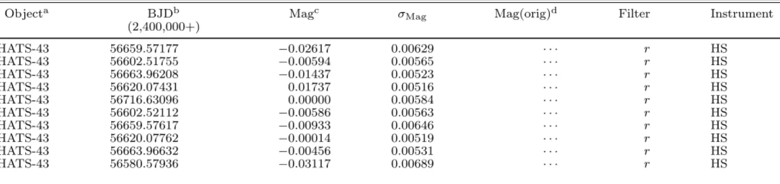
(14) 14. Brahm et al. Table 3 Light curve data for HATS-43, HATS-44, HATS-45 and HATS-46.. Objecta. BJDb (2,400,000+). HATS-43 HATS-43 HATS-43 HATS-43 HATS-43 HATS-43 HATS-43 HATS-43 HATS-43 HATS-43. 56659.57177 56602.51755 56663.96208 56620.07431 56716.63096 56602.52112 56659.57617 56620.07762 56663.96632 56580.57936. Magc. σMag. −0.02617 −0.00594 −0.01437 0.01737 0.00000 −0.00586 −0.00933 −0.00014 −0.00456 −0.03117. 0.00629 0.00565 0.00523 0.00516 0.00584 0.00563 0.00646 0.00519 0.00531 0.00689. Mag(orig)d. Filter. ··· ··· ··· ··· ··· ··· ··· ··· ··· ···. r r r r r r r r r r. Instrument HS HS HS HS HS HS HS HS HS HS. Note. — This table is available in a machine-readable form in the online journal. A portion is shown here for guidance regarding its form and content. a Either HATS-43, HATS-44, HATS-45 or HATS-46. b Barycentric Julian Date is computed directly from the UTC time without correction for leap seconds. c The out-of-transit level has been subtracted. For observations made with the HATSouth instruments (identified by “HS” in the “Instrument” column) these magnitudes have been corrected for trends using the EPD and TFA procedures applied prior to fitting the transit model. This procedure may lead to an artificial dilution in the transit depths. The blend factors for the HATSouth light curves are listed in Table 5. For observations made with follow-up instruments (anything other than “HS” in the “Instrument” column), the magnitudes have been corrected for a quadratic trend in time, and for variations correlated with up to three PSF shape parameters, fit simultaneously with the transit. d Raw magnitude values without correction for the quadratic trend in time, or for trends correlated with the seeing. These are only reported for the follow-up observations. HATS-44 0.0. 0.5. 0.5. 1.0. 1.0. 1.5. 1.5. 3. ρ* [g/cm ]. 3. ρ* [g/cm ]. HATS-43 0.0. 2.0 2.5. 2.0 2.5. 3.0. 3.0. 3.5. 3.5. 4.0. 4.0. 4.5. 4.5 5400. 5200. 5000. 4800. 4600. 5400. 5200. Effective temperature [K]. 5000. 4800. 4600. Effective temperature [K]. HATS-45. HATS-46. 0.0. 0.0. 0.2 1.0. 0.6. 3. ρ* [g/cm ]. ρ* [g/cm3]. 0.4. 0.8. 2.0. 3.0. 1.0. 1.2. 4.0. 1.4 7000. 6800. 6600. 6400. 6200. 6000. Effective temperature [K]. 5.0 6000. 5800. 5600. 5400. 5200. 5000. Effective temperature [K]. Figure 9. Model isochrones from Yi et al. (2001) for the measured metallicities of HATS-43 (upper left), HATS-44 (upper right), HATS-45 (lower left) and HATS-46 (lower right). We show models for ages of 0.2 Gyr and 1.0 to 14.0 Gyr in 1.0 Gyr increments (ages increasing from left to right). The adopted values of Teff? and ρ? are shown together with their 1σ and 2σ confidence ellipsoids. The initial values of Teff? and ρ? from the first ZASPE and light curve analyses are represented with a triangle.. • HATS-44 – similar to HATS-43, except here we can only reject blend models at 2.3σ confidence based on the photometry. The blend models which provide the best fit to the photometry (i.e., those that can be rejected with greater than 2.3σ con-. fidence based on the photometry, but which cannot be rejected with greater than 5σ confidence) have simulated RV measurements that do not resemble the observed sinusoidal RV variation. The best fit blend model has ∆χ2 = 13.4 compared to.
(15) HATS-43b–HATS-46b. 15. Table 4 Stellar parameters for HATS-43–HATS-46. Parameter. HATS-43 Value. HATS-44 Value. Astrometric properties and cross-identifications 2MASS-ID . . . . . . . . . 05220915-3058150 05371842-2758214 GSC-ID . . . . . . . . . . . GSC 7048-01851 GSC 6497-00040 R.A. (J2000) . . . . . . . 05h 22m 09.16s 05h 37m 18.41s Dec. (J2000) . . . . . . . −30◦ 580 15.000 −27◦ 580 21.400 µR.A. (mas yr−1 ) 9.8 ± 1.9 −2.2 ± 1.3 µDec. (mas yr−1 ) 7.9 ± 1.7 −3.1 ± 1.6. HATS-45 Value. HATS-46 Value. 06475862-2154385 GSC 5961-02383 06h 47m 58.63s −21◦ 540 38.500 −5.1 ± 2.5 2.8 ± 1.6. 00264858-5618580 GSC 8468-01248 00h 26m 48.58s −56◦ 180 58.000 21.3 ± 1.7 5.0 ± 1.9. 2MASS 2MASS UCAC4 UCAC4. Source. Spectroscopic properties Teff? (K). . . . . . . . . . . [Fe/H] . . . . . . . . . . . . . v sin i (km s−1 ) . . . . vmac (km s−1 ) . . . . . vmic (km s−1 ) . . . . . . γRV (m s−1 ) . . . . . . .. 5099 ± 61 0.050 ± 0.041 1.11 ± 0.82 2.948 ± 0.093 0.747 ± 0.030 22077.5 ± 8.3. 5080 ± 100 0.320 ± 0.071 0.5 ± 1.1 2.92 ± 0.15 0.737 ± 0.051 44082 ± 14. 6450 ± 110 0.020 ± 0.068 9.90 ± 0.40 5.03 1.69 19423 ± 17. 5495 ± 69 −0.060 ± 0.046 0.90 ± 0.66 3.56 ± 0.10 0.932 ± 0.033 −30192.7 ± 8.6. ZASPEa ZASPE ZASPE Assumed Assumed FEROSb. Photometric properties B (mag) . . . . . . . . . . . V (mag) . . . . . . . . . . . g (mag) . . . . . . . . . . . . r (mag) . . . . . . . . . . . . i (mag) . . . . . . . . . . . . J (mag) . . . . . . . . . . . H (mag) . . . . . . . . . . . Ks (mag) . . . . . . . . . .. 14.471 ± 0.050 13.593 ± 0.030 13.973 ± 0.030 13.301 ± 0.020 13.094 ± 0.070 12.064 ± 0.026 11.646 ± 0.022 11.556 ± 0.023. 15.487 ± 0.020 14.428 ± 0.010 14.933 ± 0.010 14.086 ± 0.010 13.794 ± 0.030 12.699 ± 0.023 12.234 ± 0.022 12.188 ± 0.030. 13.845 ± 0.020 13.307 ± 0.050 13.550 ± 0.020 13.201 ± 0.060 13.162 ± 0.040 12.364 ± 0.024 12.155 ± 0.024 12.137 ± 0.021. 14.421 ± 0.010 13.634 ± 0.050 14.018 ± 0.010 13.487 ± 0.020 13.45 ± 0.22 12.366 ± 0.024 11.993 ± 0.022 11.965 ± 0.024. APASSc APASSc APASSc APASSc APASSc 2MASS 2MASS 2MASS. 0.837 ± 0.023 0.812 ± 0.032 4.539 ± 0.036 1.96 ± 1.00 2.18+0.36 −0.20 0.400 ± 0.046 5.97 ± 0.14 3.91 ± 0.10 8.6+3.0 −4.8 0.000 ± 0.018 341 ± 17. 0.860 ± 0.021 0.847 ± 0.036 4.514 ± 0.036 1.59+0.46 −0.28 1.98 ± 0.25 0.400 ± 0.051 6.01 ± 0.16 3.85 ± 0.11 9.7+2.4 −4.0 0.095 ± 0.064 463 ± 23. 1.272 ± 0.048 1.315 ± 0.064 4.305 ± 0.036 0.81+0.16 −0.11 0.79 ± 0.10 2.66 ± 0.36 3.68 ± 0.16 2.58 ± 0.11 1.52 ± 0.70 0.042+0.106 −0.042 818 ± 41. 0.917 ± 0.027 0.853+0.040 −0.030 4.542 ± 0.038 3.20 ± 0.72 2.10+0.22 −0.29 0.589 ± 0.070 5.47 ± 0.14 3.704 ± 0.098 3.0+3.4 −2.1 0.000 ± 0.013 448 ± 22. YY+ρ? +ZASPE d YY+ρ? +ZASPE YY+ρ? +ZASPE Light curves YY+Light curves+ZASPE YY+ρ? +ZASPE YY+ρ? +ZASPE YY+ρ? +ZASPE YY+ρ? +ZASPE YY+ρ? +ZASPE YY+ρ? +ZASPE. Derived properties M? (M ) . . . . . . . . . . R? (R ) . . . . . . . . . . . log g? (cgs) . . . . . . . . ρ? (g cm−3 ) e . . . . . . ρ? (g cm−3 ) e . . . . . . L? (L ) . . . . . . . . . . . MV (mag) . . . . . . . . . MK (mag,ESO). . . . Age (Gyr) . . . . . . . . . AV (mag) . . . . . . . . . Distance (pc) . . . . . .. Note. — For HATS-43 we adopt a model in which the eccentricity is allowed to vary. For the other three systems we adopt a model in which the orbit is assumed to be circular. See the discussion in Section 3.3. a ZASPE = Zonal Atmospherical Stellar Parameter Estimator routine for the analysis of high-resolution spectra (Brahm et al. 2017b), applied to the FEROS spectra of each system. These parameters rely primarily on ZASPE, but have a small dependence also on the iterative analysis incorporating the isochrone search and global modeling of the data. b The error on γ RV is determined from the orbital fit to the RV measurements, and does not include the systematic uncertainty in transforming the velocities to the IAU standard system. The velocities have not been corrected for gravitational redshifts. c From APASS DR6 for as listed in the UCAC 4 catalog (Zacharias et al. 2012). d YY+ρ +ZASPE = Based on the YY isochrones (Yi et al. 2001), ρ as a luminosity indicator, and the ZASPE results. ? ? e In the case of ρ we list two values. The first value is determined from the global fit to the light curves and RV data, without imposing ? a constraint that the parameters match the stellar evolution models. The second value results from restricting the posterior distribution to combinations of ρ? +Teff? +[Fe/H] that match to a YY stellar model.. the adopted planetary orbit model, when including jitter in the uncertainties, and, based on an F-test, can be rejected with 99.7% confidence. Combining the RVs and photometry, all blend models can be rejected with greater than 4σ confidence. • HATS-45 – similar to HATS-43, except here we can only reject blend models at 1.4σ confidence based on the photometry alone. However, for blend models that cannot be rejected with at least 5σ confidence based on the photometry, both the simulated BSs and RVs vary by more than 500 m s−1 , and in most cases by well over 1 km s−1 (compared to the measured scatter of 36 m s−1 and 61 m s−1 for the. FEROS BS and RV values –including the planetary signal– of this target, respectively, and compared to the measured scatter of 104 m s−1 and 73 m s−1 for the HARPS BS and RV values, respectively). • HATS-46 – similar to HATS-43, in this case all blend models tested can be rejected with 2.4σ confidence based solely on the photometry. For blend models that cannot be rejected with at least 4σ confidence based on the photometry, both the simulated BSs and RVs vary by more than 200 m s−1 (compared to the measured scatter of 35 m s−1 and 39 m s−1 for the FEROS BS and RV values of this target, respectively)..
(16) 16. Brahm et al.. 3.3. Global modeling of the data In order to obtain the orbital and physical parameters of the planets we simultaneously modelled for each system the HATSouth photometry, the follow-up photometry, and the high-precision RV measurements following Pál et al. (2008); Bakos et al. (2010); Hartman et al. (2012). Photometric light curves are modelled using the Mandel & Agol (2002) models. For HATSouth light curves, we consider a dilution factor for the transit depth that compensates the blending effect produced by the presence of neighboring stars, and also the possible overcorrection introduced by the trend-filtered algorithm. In the case of the follow-up light curves, systematic trends for each event are corrected by including a timedependent quadratic signal to the transit model, and a linear signal with up to three parameters describing the shape of the PSF. Radial velocity data are modeled using Keplerian orbits, where we consider independent zero-points and RV jitter factors for each instrument, which are allowed to vary in the fit. We fitted the four systems by considering two possible cases, the eccentricity as a free parameter, and also by forcing circular orbits. For each system we estimated the Bayesian evidence of each scenario by using the method presented in Weinberg et al. (2013). We find that for HATS-43 the free-eccentricity model with e = 0.173±0.089 has a significantly higher evidence compared to the model with fixed eccentricity. For HATS-44 and HATS-45 the Bayesian evidence for the free-eccentricity models are slightly higher than for the fixed circular orbit models, however in both cases these results are generated by outlier radial velocity points. For both of these systems we therefore adopt the fixed circular orbit solutions, but note that the eccentricities are poorly constrained by the observations, with 95% confidence upper limits of e < 0.279, and e < 0.240, respectively. For HATS-46 we find that the fixed circular orbit model has higher Bayesian evidence, and we adopt the parameters from that model for this system as well. The 95% confidence upper limit on the eccentricity for HATS-46 is e < 0.559. We used a Differential Evolution Markov Chain Monte Carlo procedure to explore the fitness landscape and to determine the posterior distribution of the parameters. The resulting parameters and uncertainties for each system are listed in Table 5 and summarised below:. • HATS-43b has a Saturn-like mass of Mp = 0.261 ± 0.054 MJ , and a radius of Rp = 1.180 ± 0.050 RJ , which results in relatively low density of ρp = +0.054 0.191−0.038 g cm−3 . Its orbit is moderately eccentric and due to the low luminosity of its K-type host star HATS-43b has a rather warm equilibrium temperature of Teq = 1003 ± 27 K. • HATS-44b has a sub-Jupiter mass of Mp = 0.56 ± 0.11 MJ , and a radius of Rp = 1.067+0.125 −0.071 RJ , which results in a density of ρp = 0.56±0.19 g cm−3 . Even though the luminosities of HATS-43 and HATS-44 are similar, the smaller semi-major axis of HATS44b results in a higher equilibrium temperature of Teq = 1161 ± 34 K.. • HATS-45b has also a sub-Jupiter mass of Mp = 0.70 ± 0.15 MJ , and an inflated radius of Rp = 1.286 ± 0.093 RJ , which results in a density of ρp = −3 0.41+0.16 . HATS-45b suffers from moder−0.11 g cm ately strong irradiation from its F-type host star, which produces a high equilibrium temperature of Teq = 1518 ± 45 K. • HATS-46b has a mass of Mp = 0.173 ± 0.062 MJ which lies in the Neptune-Saturn mass range. We measured a radius of Rp = 1.286 ± 0.093 RJ for HATS-46b which combined with the mass gives a density of ρp = 0.28 ± 0.12 g cm−3 . The low luminosity of the host star produces a relatively low equilibrium temperature of Teq = 1054 ± 29 K for HATS-46b. 4. DISCUSSION. We have presented the discovery of four new short period transiting systems from the HATSouth network. The systems were identified as planetary candidates using HATSouth photometric light curves and then confirmed as planetary mass objects by measuring precise radial velocities for the host stars. The precision of the transit parameters was also improved by using additional follow-up light curves obtained with 1m-class telescopes. We found that the four planets have orbital periods shorter than 5 days and masses in the Neptune to Jupiter mass range, but all of them show radii similar to that of Jupiter. These four new systems add to the valuable population of extrasolar planets transiting stars with precisely determined masses and radii. In the top panel of Figure 10 we show the planet radius as a function of the planet mass for the population of transiting planets with uncertainties in Mp and Rp at the level of 35%, and we have included our four new systems. The lower panel of Figure 10 uses the same population of planets but in this case we plot the Teq –Mp diagram. While both diagrams show that the physical properties of HATS-43b to HATS-46b are consistent with what is expected based on the distribution of known transiting planets, we can point out a few interesting properties. 4.1. HATS-43b. With a mass of Mp = 0.261 ± 0.054 MJ and an equilibrium temperature of Teq = 1003 ± 27 K that lies close to the 1000 K limit proposed by Kovács et al. (2010) below which planet radius is not expected to be strongly affected by stellar insolation, this planet has a radius of Rp = 1.180 ± 0.050 RJ , which is particularly large if compared with other systems with similar properties. We can identify four other systems having masses and irradiation levels consistent with the ones of HATS-43b, namely HAT-P-19b (Hartman et al. 2011), WASP-29b (Hellier et al. 2010), WASP-69b (Anderson et al. 2014), and HATS-5b (Zhou et al. 2014). The properties of these systems are summarised in Table 6. HATS-43b has the largest radius of this subsample. Even though the metallicity of HATS-43 is the lowest one, which could hint to 1 query to exoplanets.eu for systems having reported values of R? , Teff , [Fe/H], and a.
(17) HATS-43b–HATS-46b. 17. Table 5 Orbital and planetary parameters for HATS-43b–HATS-46b. Parameter. HATS-43b Value. HATS-44b Value. HATS-45b Value. HATS-46b Value. Light curve parameters P (days) . . . . . . . . . . . . . . . . . . . . . Tc (BJD) a . . . . . . . . . . . . . . . . . . . T14 (days) a . . . . . . . . . . . . . . . . . . T12 = T34 (days) a . . . . . . . . . . . a/R? . . . . . . . . . . . . . . . . . . . . . . . . . ζ/R? b . . . . . . . . . . . . . . . . . . . . . . . Rp /R? . . . . . . . . . . . . . . . . . . . . . . . b2 . . . . . . . . . . . . . . . . . . . . . . . . . . . . b ≡ a cos i/R? . . . . . . . . . . . . . . . . i (deg) . . . . . . . . . . . . . . . . . . . . . . .. 4.3888497 ± 0.0000059 2457636.08946 ± 0.00025 0.12452 ± 0.00090 0.01666 ± 0.00070 13.04+0.68 −0.41 18.519 ± 0.075 0.1492 ± 0.0017 0.029+0.046 −0.018 0.172+0.104 −0.066 89.24+0.29 −0.41. 2.7439004 ± 0.0000032 2456931.11384 ± 0.00061 0.0688 ± 0.0017 0.029 ± 0.034 9.24 ± 0.38 42.0+3.3 −1.7 0.129 ± 0.010 0.743+0.051 −0.035 0.862+0.029 −0.021 84.65 ± 0.38. 4.1876244 ± 0.0000056 2456731.19533 ± 0.00073 0.1269 ± 0.0021 0.0207 ± 0.0023 9.02 ± 0.39 18.65 ± 0.25 0.1004 ± 0.0042 0.475+0.049 −0.060 0.689+0.034 −0.045 85.61 ± 0.42. 4.7423729 ± 0.0000049 2457376.68539 ± 0.00060 0.1014 ± 0.0019 0.0157 ± 0.0017 13.55+0.45 −0.65 23.21 ± 0.28 0.1088 ± 0.0027 0.402+0.055 −0.042 0.634+0.042 −0.034 87.32+0.22 −0.31. HATSouth blend factors d Blend factor . . . . . . . . . . . . . . . . . .. 1.0. 1.0. 0.810 ± 0.075. 0.877 ± 0.061, 0.863 ± 0.068. Limb-darkening coefficients e c1 , g . . . . . . . . . . . . . . . . . . . . . . . . . . c2 , g . . . . . . . . . . . . . . . . . . . . . . . . . . c1 , r . . . . . . . . . . . . . . . . . . . . . . . . . . c2 , r . . . . . . . . . . . . . . . . . . . . . . . . . . c1 , i . . . . . . . . . . . . . . . . . . . . . . . . . . c2 , i . . . . . . . . . . . . . . . . . . . . . . . . . .. ··· ··· 0.5115 0.2239 0.3873 0.2588. 0.8140 0.0272 0.5603 0.1933 0.4195 0.2444. ··· ··· 0.2511 0.3818 0.1791 0.3719. ··· ··· 0.4078 0.2935 0.3112 0.3042. RV parameters K (m s−1 ) . . . . . . . . . . . . . . . . . . . . e f ............................ ω (deg) . . . . . . . . . . . . . . . . . . . . . . . √ e cos ω . . . . . . . . . . . . . . . . . . . . . . √ e sin ω . . . . . . . . . . . . . . . . . . . . . . e cos ω . . . . . . . . . . . . . . . . . . . . . . . . e sin ω . . . . . . . . . . . . . . . . . . . . . . . . RV jitter FEROS (m s−1 ) g . . . RV jitter HARPS (m s−1 ) . . . . RV jitter PFS (m s−1 ) . . . . . . . .. 37.5 ± 8.0 0.173 ± 0.089 330 ± 120 0.38+0.11 −0.21 −0.141+0.130 −0.079 0.159+0.092 −0.121 −0.060+0.056 −0.035 20.3 ± 7.8 0 ± 10 ···. 90 ± 17 < 0.279 ··· ··· ··· ··· ··· 49 ± 11 ··· ···. 75 ± 16 < 0.240 ··· ··· ··· ··· ··· 47 ± 20 0.0 ± 5.4 ···. Planetary parameters Mp (MJ ) . . . . . . . . . . . . . . . . . . . . . Rp (RJ ) . . . . . . . . . . . . . . . . . . . . . . C(Mp , Rp ) h . . . . . . . . . . . . . . . . . ρp (g cm−3 ) . . . . . . . . . . . . . . . . . . log gp (cgs) . . . . . . . . . . . . . . . . . . . a (AU) . . . . . . . . . . . . . . . . . . . . . . . Teq (K) . . . . . . . . . . . . . . . . . . . . . . Θ i ........................... log10 hF i (cgs) j . . . . . . . . . . . . . .. 0.261 ± 0.054 1.180 ± 0.050 −0.01 0.191+0.054 −0.038 2.67 ± 0.11 0.04944 ± 0.00046 1003 ± 27 0.0265 ± 0.0057 8.359 ± 0.047. 0.56 ± 0.11 1.067+0.125 −0.071 0.01 0.56 ± 0.19 3.08 ± 0.13 0.03649 ± 0.00030 1161 ± 34 0.0438 ± 0.0095 8.613 ± 0.051. 0.70 ± 0.15 1.286 ± 0.093 0.01 0.41+0.16 −0.11 3.02 ± 0.12 0.05511 ± 0.00069 1518 ± 45 0.047 ± 0.011 9.079 ± 0.051. 22.1 ± 8.0 < 0.559 ··· ··· ··· ··· 32.9 ± 6.7 ··· 22.7 ± 6.8 0.173 ± 0.062 0.903+0.058 −0.045 −0.02 0.28 ± 0.12 2.71+0.14 −0.20 0.05367 ± 0.00053 1054 ± 29 0.0222 ± 0.0082 8.445 ± 0.048. Note. — For HATS-43 we adopt a model in which the eccentricity is allowed to vary. For the other three systems we adopt a model in which the orbit is assumed to be circular. See the discussion in Section 3.3. a Times are in Barycentric Julian Date calculated directly from UTC without correction for leap seconds. T : Reference epoch of mid transit that c minimizes the correlation with the orbital period. T12 : total transit duration, time between first to last contact; T12 = T34 : ingress/egress time, time between first and second, or third and fourth contact. b Reciprocal of the half duration of the transit used as a jump parameter in our MCMC analysis in place of a/R . It is related to a/R by the ? ? √ √ expression ζ/R? = a/R? (2π(1 + e sin ω))/(P 1 − b2 1 − e2 ) (Bakos et al. 2010). d Scaling factor applied to the model transit that is fit to the HATSouth light curves. This factor accounts for dilution of the transit due to blending from neighboring stars and over-filtering of the light curve. These factors are varied in the fit. For HATS-43 and HATS-44 we fix these values to one because the analysis is performed on light curves after applying signal-reconstruction TFA to correct for over-filtering. For HATS-46 we list separately the dilution factors adopted for the G755.2 and G754.3 HATSouth light curves. e Values for a quadratic law, adopted from the tabulations by Claret (2004) according to the spectroscopic (ZASPE) parameters listed in Table 4. f For fixed circular orbit models we list the 95% confidence upper limit on the eccentricity determined when √e cos ω and √e sin ω are allowed to vary in the fit. g Term added in quadrature to the formal RV uncertainties for each instrument. This is treated as a free parameter in the fitting routine. In cases where the jitter is consistent with zero, we list its 95% confidence upper limit. h Correlation coefficient between the planetary mass M and radius R estimated from the posterior parameter distribution. p p 2 i The Safronov number is given by Θ = 1 (V esc /Vorb ) = (a/Rp )(Mp /M? ) (see Hansen & Barman 2007). 2 j Incoming flux per unit surface area, averaged over the orbit..
(18) 18. Brahm et al.. 2.0 2400 2100. RP [RJ ]. 1.5. 1.0. Jupiter. HS-45 HS-43 HS-44. Saturn. HS-46. 1800 1500. Teq [K]. 1200 HS-7. 0.5. 900. Neptune. 0.0 -3 10. 600 300 10 -1. 10 -2. MP [MJ ]. 10 1. 10 0. 10 2. 2.0 10 1. RP [RJ ]. 1.5 10 0. HS-45 HS-43 HS-44. 1.0. MP [MJ ]. HS-46. 10 -1. 0.5 10 -2 0.0. 0. 500. 1000. 1500. Teq [K]. 2000. 2500. 3000. Figure 10. Top: Planetary mass–radius diagram for the population of well characterised planets with masses and radii measured at the 35% level. The planetary equilibrium temperature is colour coded. The big circles with error bars correspond to HATS-43b, HATS-44b, HATS-45b, and HATS-46b. The plotted lines correspond to the Fortney et al. (2007) models for irradiated planets at 0.045 AU from the host star. The black lines represent planets with an age of 1 Gyr, while light blue lines represent planet with an age of 4.5 Gyr. From top to bottom the models contain core masses of 0, 10, 25 and 50 earth masses. Bottom: Planet radius as a function of the equilibrium temperature for the same systems considered in the upper panel. The dashed grey line corresponds to the temperature limit below which inflation mechanisms of hot Jupiters are not expected to play a major role. While the radii for HATS-44b, HATS-45b, and HATS-46b clearly follow the empirical trend of increasing radius with the insolation level, HATS-43b has a slightly larger radius that the one predicted from this empirical correlation..
(19) HATS-43b–HATS-46b the absence of a central solid core and consequently a larger radius, the Fortney et al. (2007) models of planetary structure predict a radius that is more than 2σ below the adopted value for HATS-43b. On the other hand, HATS-43b stands out as the only system of the subsample having an eccentricity greater than 0.1. Given that the physical properties of the stellar hosts of Table 6 are similar, this enhanced eccentricity directly translates in a greater tidal heating rate (Jackson et al. 2008) that could be the driving source responsible for the large radius of HATS-43b. The low density of HATS-43b makes this system an interesting target for atmospheric studies. Specifically, its expected transmission spectroscopy signal of δtrans = 2350 ppm, is among the highest values form the full population of discovered transiting systems. WASP-39b (Faedi et al. 2011), which has a similar transmission spectroscopy signal (δtrans = 2500 ppm) and similar physical properties to HATS-43b, has been the target of numerous atmospheric studies (Kammer et al. 2015; Fischer et al. 2016; Nikolov et al. 2016) that find that this planet has a cloud free atmosphere with presence of Rayleigh scattering slope and Na and K absorption lines. HATS-43b is a well suited comparison target to study the atmospheres of Saturn mass planets with even lower temperatures. 4.2. HATS-44b & HATS-45b. HATS-44b with a mass of Mp = 0.56±0.11 MJ and a ra+0.125 dius of Rp = 1.067−0.071 RJ , and HATS-45b with a mass of Mp = 0.70±0.15 MJ and a radius of Rp = 1.286±0.093 RJ are, two sub-Jupiter mass planets that lie in relatively densely populated regions of the parameter space of transiting systems (see Figure 10). The most similar system to HATS-44b in terms of planet mass and irradiation level, is WASP-34 (Mp =0.59±0.01 MJ , Teq =1160 K Smalley et al. 2011), which has a slightly larger radius of Rp =1.22±0.10 RJ which is in agreement with the proposed anti correlation between the planet radius and the metallicity of the host start. WASP-34b has a moderately metal poor stellar host star ([Fe/H]=-0.02±0.10) if compared to HATS-44 ([Fe/H]=+0.32±0.07). In the case of HATS-45b, the most similar system is HAT-P-9b (Mp =0.78±0.09 MJ , Teq =1530 ± 40 K, Shporer et al. 2009), which presents a significantly inflated radius of Rp =1.4 ± 0.06 RJ , slightly larger but consistent with the one of HATS-45b. While the radius of HATS-44b can be predicted by using the Fortney et al. (2007) models invoking a core-less structure, the radius of HATS-45b is larger than predicted, which can be expected due to the moderately high irradiation from its F-type host star, where some of the proposed inflation mechanisms of hot Jupiters might be in play. Even though both planets have expected transmission signals significantly smaller than HATS-43b (δtrans = 860 ppm and δtrans = 660 ppm, for HATS-44b and HATS-45b, respectively), there have been previous atmospheric studies of transiting planets with similar values of transmission signal (e.g. Parviainen et al. 2016; von Essen et al. 2017). Additionally, the v sin i = 9.90±0.40 km s−1 of HATS-45 makes of this system and interesting target for the determination of the obliquity through the measurement of the Rossiter-McLaughlin effect. The ex-. 19. pected semi-amplitude of the radial velocity anomaly for an aligned orbit is of KRM = 30 m s−1 . 4.3. HATS-46b Having a mass of Mp = 0.173 ± 0.062 MJ , HATS-46b lies in the sparsely populated region of the parameter space of transiting systems in the Neptune – Saturn mass range, which corresponds to the transition zone between ice giants and gas giants. According to the core accretion theory of giant planet formation (Pollack et al. 1996), planetesimals agglomerate to form rocky embryos that when reaching a threshold mass of ∼10 M⊕ , generate a run away accretion of the surrounding gas of the protoplanetary disk that forms thick H/He dominated envelope (90% in mass). One of the theoretical challenges of this model is to understand how ice giants (like Uranus and Neptune) can avoid the accretion of the massive gaseous envelope. For this reason, the discovery of transiting planets in the ice–gas transition range is important for determining which properties of the systems can play a major role in setting their structure and composition, which can be then linked to different formation models. The large radius of HATS-46b suggest that this planet is probably a low mass gas giant planet, and not a high mass ice giant. By using the Fortney et al. (2007) models of planetary structure we find that HATS-46b should have a core mass of Mc =12±8 M⊕ to explain its mass and radius, implying a ∼ 80% H/He dominated composition. Among the population of discovered transiting systems orbiting main sequence stars with precise mass estimations from RVs, we can identify Kepler-89d (0.16 MJ , 0.98 RJ , Weiss et al. 2013), HATS-8b (0.14 MJ , 0.87 RJ , Bayliss et al. 2015) HAT-P-48b, (0.17 MJ , 1.30 RJ , Bakos et al. 2016), WASP-139b (0.12 MJ , 0.80 RJ , Hellier et al. 2017), and WASP-107b (0.12 MJ , 0.94 RJ , Anderson et al. 2017) as other similar low mass gas giants, while Kepler-101b (0.16 MJ , 0.51 RJ , Bonomo et al. 2014), HATS-7b (0.12 MJ , 0.56 RJ , Bakos et al. 2015), K2-98b (0.10 MJ , 0.38 RJ , Barragán et al. 2016), and K2-27b (0.10 MJ , 0.40 RJ , Petigura et al. 2017) are compatible with being high mass ice giants. These two groups of planets can be associated to different locations and/or times of formation. The first group of planets could have been formed relatively close to the host star where the high temperature prevents the formation of icy planetesimals that pollute the planet composition. On the other hand, the second group of planets could have formed farther away or early in the disk lifetime where rocky planetesimals are still present in profusion. This suggested simple classification of these ten planets is based on the amount of heavy elements inferred from classical models of planetary structure, but there are several additional factors that are not taken into account that can contribute to modify the planetary radius and mislead the determination of the planet metallicity, e.g. evaporation (Owen & Wu 2013), tidal heating (Jackson et al. 2008), or collisions with other planets (Liu et al. 2015). On the other hand, studies of atmospheric composition can be used to directly discriminate if these planets have H/He dominated envelopes or if there is a significant presence of heavier elements, as was recently shown by Wakeford et al. (2017), where a significantly metal depleted composition was estimated for the Neptune mass planet HAT-P-26b. In this context, HATS-46b has a.
(20) 20. Brahm et al. Table 6 Discovered transiting planets having reported Mp and Teq values consistent with HATS-43b. a. Name. Mp [MJ ]. Teq [K]. Rp [RJ ]. [Fe/H] [dex]. e. H [1019 W]a. WASP-29b WASP-69b HAT-P-19b HATS-5b. 0.244 ± 0.020 0.260 ± 0.017 0.292 ± 0.020 0.237 ± 0.012. 980 ± 40 963 ± 18 1010 ± 42 1025 ± 17. 0.792+0.056 −0.035 1.057 ± 0.047 1.132 ± 0.072 0.912 ± 0.025. +0.11 ± 0.14 +0.15 ± 0.08 +0.23 ± 0.08 +0.19 ± 0.08. 0.03+0.05 −0.03 < 0.1 at 2σ 0.067 ± 0.042 0.019 ± 0.019. 1.18 < 16 14 0.2. HATS-43b. 0.261 ± 0.054. 1003 ± 27. 1.180 ± 0.050. +0.050 ± 0.041. 0.173 ± 0.089. 52. Tidal heating rate (Jackson et al. 2008).. prominent expected transmission signal of ∼1500 ppm, which should make of this system a valuable target for atmospheric studies. Development of the HATSouth project was funded by NSF MRI grant NSF/AST-0723074, operations have been supported by NASA grants NNX09AB29G, NNX12AH91H, and NNX17AB61G, and follow-up observations receive partial support from grant NSF/AST1108686. J.H. acknowledges support from NASA grant NNX14AE87G. A.J. acknowledges support from FONDECYT project 1171208, BASAL CATA PFB-06, and project IC120009 “Millennium Institute of Astrophysics (MAS)” of the Millenium Science Initiative, Chilean Ministry of Economy. N.E. is supported by BASAL CATA PFB-06. R.B. and N.E. acknowledge support from project IC120009 “Millenium Institute of Astrophysics (MAS)” of the Millennium Science Initiative, Chilean Ministry of Economy. V.S. acknowledges support form BASAL CATA PFB-06. This work is based on observations made with ESO Telescopes at the La Silla Observatory. This paper also uses observations obtained with facilities of the Las Cumbres Observatory Global Telescope. We acknowledge the use of the AAVSO Photometric All-Sky Survey (APASS), funded by the Robert Martin Ayers Sciences Fund, and the SIMBAD database, operated at CDS, Strasbourg, France. Operations at the MPG 2.2 m Telescope are jointly performed by the Max Planck Gesellschaft and the European Southern Observatory. The imaging system GROND has been built by the high-energy group of MPE in collaboration with the LSW Tautenburg and ESO. We thank the MPG 2.2m telescope support team for their technical assistance during observations..
(21) HATS-43b–HATS-46b REFERENCES Anderson, D. R., Collier Cameron, A., Delrez, L., et al. 2014, MNRAS, 445, 1114 —. 2017, ArXiv e-prints, 1701.03776 Bakos, G., Noyes, R. W., Kovács, G., et al. 2004, PASP, 116, 266 Bakos, G. Á., Torres, G., Pál, A., et al. 2010, ApJ, 710, 1724 Bakos, G. Á., Csubry, Z., Penev, K., et al. 2013, PASP, 125, 154 Bakos, G. Á., Penev, K., Bayliss, D., et al. 2015, ApJ, 813, 111 Bakos, G. Á., Hartman, J. D., Torres, G., et al. 2016, ArXiv e-prints, 1606.04556 Baranne, A., Queloz, D., Mayor, M., et al. 1996, A&AS, 119, 373 Barragán, O., Grziwa, S., Gandolfi, D., et al. 2016, AJ, 152, 193 Batygin, K., & Stevenson, D. J. 2010, ApJ, 714, L238 Bayliss, D., Zhou, G., Penev, K., et al. 2013, AJ, 146, 113 Bayliss, D., Hartman, J. D., Bakos, G. Á., et al. 2015, AJ, 150, 49 Bhatti, W., Bakos, G. Á., Hartman, J. D., et al. 2016, ArXiv e-prints, 1607.00322 Bonomo, A. S., Sozzetti, A., Lovis, C., et al. 2014, A&A, 572, A2 Brahm, R., Jordán, A., & Espinoza, N. 2017a, PASP, 129, 034002 Brahm, R., Jordán, A., Hartman, J., & Bakos, G. 2017b, MNRAS, 467, 971 Brahm, R., Jordán, A., Bakos, G. Á., et al. 2016, AJ, 151, 89 Brown, T. M., Baliber, N., Bianco, F. B., et al. 2013, PASP, 125, 1031 Burrows, A., Hubeny, I., Budaj, J., & Hubbard, W. B. 2007, ApJ, 661, 502 Butler, R. P., Marcy, G. W., Williams, E., et al. 1996, PASP, 108, 500 Claret, A. 2004, A&A, 428, 1001 Crane, J. D., Shectman, S. A., Butler, R. P., et al. 2010, in Society of Photo-Optical Instrumentation Engineers (SPIE) Conference Series, Vol. 7735, Society of Photo-Optical Instrumentation Engineers (SPIE) Conference Series Dawson, R. I., & Murray-Clay, R. A. 2013, ApJ, 767, L24 Dopita, M., Hart, J., McGregor, P., et al. 2007, Ap&SS, 310, 255 Espinoza, N., Bayliss, D., Hartman, J. D., et al. 2016, AJ, 152, 108 Faedi, F., Barros, S. C. C., Anderson, D. R., et al. 2011, A&A, 531, A40 Fischer, P. D., Knutson, H. A., Sing, D. K., et al. 2016, ApJ, 827, 19 Fortney, J. J., Marley, M. S., & Barnes, J. W. 2007, ApJ, 659, 1661 Fraine, J., Deming, D., Benneke, B., et al. 2014, Nature, 513, 526 Girardi, L., Bressan, A., Bertelli, G., & Chiosi, C. 2000, A&AS, 141, 371 Hansen, B. M. S., & Barman, T. 2007, ApJ, 671, 861 Hartman, J. D., Bakos, G. Á., Sato, B., et al. 2011, ApJ, 726, 52 Hartman, J. D., Bakos, G. Á., Béky, B., et al. 2012, AJ, 144, 139 Hartman, J. D., Bayliss, D., Brahm, R., et al. 2015, AJ, 149, 166 Hartman, J. D., Bakos, G. Á., Bhatti, W., et al. 2016, AJ, 152, 182 Hellier, C., Anderson, D. R., Collier Cameron, A., et al. 2010, ApJ, 723, L60 Hellier, C., Anderson, D. R., Cameron, A. C., et al. 2017, MNRAS, 465, 3693. 21. Hippler, S., Bergfors, C., Brandner Wolfgang, et al. 2009, The Messenger, 137, 14 Howell, S. B., Sobeck, C., Haas, M., et al. 2014, PASP, 126, 398 Jackson, B., Greenberg, R., & Barnes, R. 2008, ApJ, 681, 1631 Janson, M., Durkan, S., Hippler, S., et al. 2017, A&A, 599, A70 Jordán, A., Brahm, R., Bakos, G. Á., et al. 2014, AJ, 148, 29 Kammer, J. A., Knutson, H. A., Line, M. R., et al. 2015, ApJ, 810, 118 Kaufer, A., & Pasquini, L. 1998, in Society of Photo-Optical Instrumentation Engineers (SPIE) Conference Series, Vol. 3355, Optical Astronomical Instrumentation, ed. S. D’Odorico, 844–854 Kovács, G., Bakos, G., & Noyes, R. W. 2005, MNRAS, 356, 557 Kovács, G., Zucker, S., & Mazeh, T. 2002, A&A, 391, 369 Kovács, G., Bakos, G. Á., Hartman, J. D., et al. 2010, ApJ, 724, 866 Liu, S.-F., Hori, Y., Lin, D. N. C., & Asphaug, E. 2015, ApJ, 812, 164 Mandel, K., & Agol, E. 2002, ApJ, 580, L171 Mayor, M., Pepe, F., Queloz, D., et al. 2003, The Messenger, 114, 20 Mordasini, C., Alibert, Y., Georgy, C., et al. 2012, A&A, 547, A112 Nikolov, N., Sing, D. K., Gibson, N. P., et al. 2016, ApJ, 832, 191 Owen, J. E., & Wu, Y. 2013, ApJ, 775, 105 Pál, A., Bakos, G. Á., Torres, G., et al. 2008, ApJ, 680, 1450 Parviainen, H., Pallé, E., Nortmann, L., et al. 2016, A&A, 585, A114 Penev, K., Bakos, G. Á., Bayliss, D., et al. 2013, AJ, 145, 5 Petigura, E. A., Sinukoff, E., Lopez, E. D., et al. 2017, AJ, 153, 142 Pollacco, D. L., Skillen, I., Collier Cameron, A., et al. 2006, PASP, 118, 1407 Pollack, J. B., Hubickyj, O., Bodenheimer, P., et al. 1996, Icarus, 124, 62 Ricker, G. R., Winn, J. N., Vanderspek, R., et al. 2014, in Proc. SPIE, Vol. 9143, Space Telescopes and Instrumentation 2014: Optical, Infrared, and Millimeter Wave, 914320 Shporer, A., Bakos, G. Á., Bouchy, F., et al. 2009, ApJ, 690, 1393 Smalley, B., Anderson, D. R., Collier Cameron, A., et al. 2011, A&A, 526, A130 Sozzetti, A., Torres, G., Charbonneau, D., et al. 2007, ApJ, 664, 1190 von Essen, C., Cellone, S., Mallonn, M., et al. 2017, ArXiv e-prints, 1703.10647 Wakeford, H. R., Sing, D. K., Kataria, T., et al. 2017, Science, 356, 628 Weinberg, M. D., Yoon, I., & Katz, N. 2013, ArXiv e-prints, 1301.3156 Weiss, L. M., Marcy, G. W., Rowe, J. F., et al. 2013, ApJ, 768, 14 Yi, S., Demarque, P., Kim, Y.-C., et al. 2001, ApJS, 136, 417 Zacharias, N., Finch, C. T., Girard, T. M., et al. 2012, VizieR Online Data Catalog, 1322, 0 Zhou, G., Bayliss, D., Penev, K., et al. 2014, ArXiv e-prints, 1401.1582 Zhou, G., Bayliss, D., Hartman, J. D., et al. 2015, ApJ, 814, L16.
Figure


+7


Documento similar