Search for direct top squark pair production in final states with two leptons in pp collisions at root s=8 TeV with the ATLAS detector

Texto completo

(1)arXiv:1403.4853v1 [hep-ex] 19 Mar 2014. EUROPEAN ORGANISATION FOR NUCLEAR RESEARCH (CERN). CERN-PH-EP-2014-014 Submitted to: JHEP. Search for direct top-squark pair production in final states with √ two leptons in pp collisions at s = 8 TeV with the ATLAS detector. The ATLAS Collaboration. Abstract A search is presented for direct top-squark pair production in final states with two leptons (elec√ trons or muons) of opposite charge using 20.3 fb−1 of pp collision data at s = 8 TeV, collected by the ATLAS experiment at the Large Hadron Collider in 2012. No excess over the Standard Model expectation is found. The results are interpreted under the separate assumptions (i) that the top squark decays to a b-quark in addition to an on-shell chargino whose decay occurs via a real or virtual W boson, or (ii) that the top squark decays to a t-quark and the lightest neutralino. A top squark with a mass between 150 GeV and 445 GeV decaying to a b-quark and an on-shell chargino is excluded at 95% confidence level for a top squark mass equal to the chargino mass plus 10 GeV, in the case of a 1 GeV lightest neutralino. Top squarks with masses between 215 (90) GeV and 530 (170) GeV decaying to an on-shell (off-shell) t-quark and a neutralino are excluded at 95% confidence level for a 1 GeV neutralino.. c 2014 CERN for the benefit of the ATLAS Collaboration..

(2) Prepared for submission to JHEP. Search for direct top-squark pair production in final √ states with two leptons in pp collisions at s = 8 TeV with the ATLAS detector. The ATLAS Collaboration. Abstract: A search is presented for direct top-squark pair production in final states with two leptons (electrons or muons) of opposite charge using 20.3 fb−1 of pp collision data at √ s = 8 TeV, collected by the ATLAS experiment at the Large Hadron Collider in 2012. No excess over the Standard Model expectation is found. The results are interpreted under the separate assumptions (i) that the top squark decays to a b-quark in addition to an on-shell chargino whose decay occurs via a real or virtual W boson, or (ii) that the top squark decays to a t-quark and the lightest neutralino. A top squark with a mass between 150 GeV and 445 GeV decaying to a b-quark and an on-shell chargino is excluded at 95% confidence level for a top squark mass equal to the chargino mass plus 10 GeV, in the case of a 1 GeV lightest neutralino. Top squarks with masses between 215 (90) GeV and 530 (170) GeV decaying to an on-shell (off-shell) t-quark and a neutralino are excluded at 95% confidence level for a 1 GeV neutralino..

(3) Contents 1 Introduction. 1. 2 The ATLAS detector. 3. 3 Monte Carlo simulations and data samples. 4. 4 Physics object selection. 5. 5 Event selection 5.1 Preselection and event variables 5.2 Leptonic mT2 selection 5.3 Hadronic mT2 selection 5.4 Multivariate analysis. 7 7 8 9 10. 6 Standard Model background determination 6.1 Background fit 6.2 Fake and non-prompt lepton background estimation 6.3 Leptonic mT2 analysis 6.4 Hadronic mT2 analysis 6.5 Multivariate analysis. 14 14 15 16 22 23. 7 Systematic uncertainties. 30. 8 Results and interpretation. 32. 9 Conclusions. 46. 10 Acknowledgements. 53. A Generator-level object and event selection. 60. 1. Introduction. Supersymmetry (SUSY) [1–9] is an extension to the Standard Model (SM) which introduces supersymmetric partners of the known fermions and bosons. For each known boson or fermion, SUSY introduces a particle with identical quantum numbers except for a difference of half a unit of spin (S). The introduction of gauge-invariant and renormalisable interactions into SUSY models can violate the conservation of baryon number (B) and lepton number (L),. –1–.

(4) resulting in a proton lifetime shorter than current experimental limits [10]. This is usually solved by assuming that the multiplicative quantum number R-parity (R), defined as R = (−1)3(B−L)+2S , is conserved. In the framework of a generic R-parity-conserving minimal supersymmetric extension of the SM (MSSM) [11–15], SUSY particles are produced in pairs where the lightest supersymmetric particle (LSP) is stable, and is a candidate for dark matter. In a large variety of models, the LSP is the lightest neutralino (χ̃01 ). The scalar partners of right-handed and left-handed quarks (squarks), q̃R and q̃L , mix to form two mass eigenstates, q̃1 and q̃2 , with q̃1 defined to be the lighter one. In the case of the supersymmetric partner of the top quark (top squark, t̃), large mixing effects can lead to one top-squark mass eigenstate, t̃1 , that is significantly lighter than the other squarks. Consideration of naturalness and its impact on the SUSY particle spectrum, suggests that top squarks cannot be too heavy, to keep the Higgs boson mass close to the electroweak scale [16, 17]. Thus t̃1 could be pair-produced with relatively large cross-sections at the Large Hadron Collider (LHC). The top squark can decay into a variety of final states, depending, amongst other factors, on the hierarchy of the mass eigenstates formed from the linear superposition of the SUSY partners of the Higgs boson and electroweak gauge bosons. In this paper the relevant mass 0 eigenstates are the lightest chargino (χ̃± 1 ) and the χ̃1 . Two possible sets of SUSY mass spectra are considered, assuming that the mixing of the neutralino gauge eigenstates is such that the χ̃01 is mostly the supersymmetric partner of the SM boson B (before electroweak symmetry breaking) and taking into account previous experimental constraints from the LEP experiments [18] that m(χ̃± 1 ) > 103.5 GeV. In both sets of spectra (figure 1) the t̃1 is the only coloured particle contributing to the production processes. In the first scenario the t̃1 , assumed to be t̃L , decays via t̃1 → b + χ̃± 1, ± ± ˜ where m(t1 ) − m(χ̃1 ) > m(b), and the χ̃1 (assumed to be mostly the supersymmetric partner of the SM W boson before electroweak symmetry breaking) subsequently decays into the lightest neutralino (assumed to be the LSP) and a real (figure 1 (a)) or virtual (figure 1 (b)) W boson. In the second scenario (figure 1 (c)), the t̃1 , assumed to be 70% t̃R , decays via t̃1 → t + χ̃01 . Both on-shell, kinematically allowed for m(t̃1 ) > m(t) + m(χ̃01 ), and off-shell (resulting in a three-body decay to bW χ̃01 ) top quarks are considered. In all scenarios the top squarks are pair-produced and, since only the leptonic decay mode of the W (∗) is considered, the events are characterised by the presence of two isolated leptons (e, µ)1 with opposite charge, and two b-quarks. Significant missing transverse momentum miss pmiss T , whose magnitude is referred to as ET , is also expected from the neutrinos and neutralinos in the final states. In this paper, three different analysis strategies are used to search for t̃1 pair production, with a variety of signal regions defined for each. Two of the analyses target the t̃1 → b + χ̃± 1 decay mode and the three-body t̃1 → bW χ̃01 decay via an off-shell top-quark, whilst one targets the t̃1 → t + χ̃01 to an on-shell top-quark decay mode. The kinematics of the t̃1 → b + χ̃± 1 decay mode depend upon the mass hierarchy of the t̃1 , 1. Electrons and muons from τ decays are included.. –2–.

(5) 0 χ̃± 1 and χ̃1 particles (figure 1 (a) and 1 (b)). In order to be sensitive to all the possible mass splittings, two complementary cut-based analysis strategies are designed: one to target large ± 0 0 χ̃± 1 − χ̃1 mass splittings (larger than the W bosons mass), and one to target small χ̃1 − χ̃1 mass splittings (smaller than the W bosons mass); the first one provides the sensitivity to the t̃1 three-body decay. These signatures have both very small cross-section and low branching ratios (BRs) (of top-quark pairs to dileptonic final states). A multivariate approach is used to target the on-shell top t̃1 → t + χ̃01 decay mode (figure 1 (c)), to enhance sensitivity beyond what can be achieved with cut-and-count techniques.. ~ t1. ~ t1. ~ t1. b ± ∼ χ1. b t (∗)(→ bℓν). W(→ ℓν). ± ∼ χ ∗. W (→ ℓν) (a). 0 ∼ χ 1. (b). 1. 0 ∼ χ 1. (c). 0 ∼ χ 1. Figure 1. Schematic diagrams of mass hierarchy for the t̃1 → b + χ̃± 1 decay mode ((a) larger than ± 0 0 the W mass (χ̃1 , χ̃1 ) mass splitting and (b) smaller than the W mass (χ̃± 1 , χ̃1 ) mass splitting), and 0 (c) the t̃1 → tχ̃1 decay mode.. √ Previous ATLAS analyses using data at s = 7 TeV and 8 TeV have placed exclusions 0 limits at 95% confidence level (CL) on both the t̃1 → b + χ̃± 1 [19–21] and t̃1 → t + χ̃1 [22–24] decay modes. This search is an update of the 7 TeV analysis targeting the two-lepton final state [24] with a larger dataset, including additional selections sensitive to various signal models and exploiting a multivariate analysis technique. Limits on top squarks direct production have also been placed by the CMS [25–28], CDF [29] and D0 [30] collaborations.. 2. The ATLAS detector. ATLAS is a multi-purpose particle physics experiment [31] at the LHC. The detector layout2 consists of inner tracking devices surrounded by a superconducting solenoid, electromagnetic 2. ATLAS uses a right-handed coordinate system with its origin at the nominal interaction point (IP) in the centre of the detector and the z-axis coinciding with the axis of the beam pipe. The x-axis points from the IP to the centre of the LHC ring, and the y-axis points upwards. Cylindrical coordinates (r, φ) are used in the transverse plane, φ being the azimuthal angle around the beam pipe. The pseudorapidity is defined in terms of the polar angle θ as η = − ln tan(θ/2).. –3–.

(6) and hadronic calorimeters and a muon spectrometer. The inner tracking detector (ID) covers |η| < 2.5 and consists of a silicon pixel detector, a semicondictor microstrip detector, and a transition radiation tracker. The ID is surrounded by a thin superconducting solenoid providing a 2T axial magnetic field and it provides precision tracking of charged particles and vertex reconstruction. The calorimeter system covers the pseudorapidity range |η| < 4.9. In the region |η| < 3.2, high-granularity liquid-argon electromagnetic sampling calorimeters are used. A steel/scintillator-tile calorimeter provides energy measurements for hadrons within |η| < 1.7. The end-cap and forward regions, which cover the range 1.5 < |η| < 4.9, are instrumented with liquid-argon calorimeters for both electromagnetic and hadronic particles. The muon spectrometer surrounds the calorimeters and consists of three large superconducting air-core toroid magnets, each with eight coils, a system of precision tracking chambers (|η| < 2.7) and fast trigger chambers (|η| < 2.4).. 3. Monte Carlo simulations and data samples. Monte Carlo (MC) simulated event samples are used to model the signal and to describe all the backgrounds which produce events with two prompt leptons from W , Z or H decays. All MC samples utilised in the analysis are produced using the ATLAS Underlying Event Tune 2B [32] and are processed through the ATLAS detector simulation [33] based on GEANT4 [34] or passed through a fast simulation using a parameterisation of the performance of the ATLAS electromagnetic and hadronic calorimeters [35]. Additional pp interactions in the same (intime) and nearby (out-of-time) bunch crossings (pile-up) are included in the simulation. Processes involving supersymmetric particles are generated using HERWIG++2.5.2 [36] (t̃1 → t+ χ̃01 ) and MADGRAPH-5.1.4.8 [37] (t̃1 → b+ χ̃± 1 ) interfaced to PYTHIA-6.426 [38] (with the PDF set CTEQ6L1 [39]). Different initial-state (ISR) and final-state radiation (FSR) and αs parameter values are used to generate additional samples in order to evaluate the effect of their systematic uncertainties. Signal cross-sections are calculated at next-to-leading order (NLO) in αs , including the resummation of soft gluon emission at next-to-leading-logarithm accuracy (NLO+NLL) [40–42], as described in ref. [43]. Top-quark pair and W t production are simulated with MC@NLO-4.06 [44, 45], interfaced with HERWIG-6.520 [46] for the fragmentation and the hadronisation processes, and using JIMMY-4.31 [47] for the underlying event description. In addition, ACERMC-3.8 [48] samples and POWHEG-1.0 [49] samples, interfaced to both PYTHIA-6.426 and HERWIG-6.520, are used to estimate the event generator, fragmentation and hadronisation systematic uncertainties. Samples of tt̄Z and tt̄W production (referred to as tt̄V ) are generated with MADGRAPH-5.1.4.8 interfaced to PYTHIA-6.426. Samples of Z/γ ? produced in association with jets are generated with SHERPA-1.4.1 [50], while ALPGEN-2.14 [51] samples are used for evaluation of systematic uncertainties. Diboson samples (W W , W Z, ZZ) are generated with POWHEG-1.0. Additional samples generated with SHERPA-1.4.1 are used to estimate the systematic arising from choice of event generator. Higgs boson production, including all decay modes,3 is simulated with 3. An SM-like 125 GeV Higgs boson, with the same BR as in the SM, is assumed.. –4–.

(7) PYTHIA-8.165 [52]. Samples generated with MC@NLO-4.06, POWHEG-1.0 and SHERPA-1.4.1 are produced using the parton distribution function (PDF) set CT10 [53]. All other samples are generated using the PDF set CTEQ6L1. The background predictions are normalised to the theoretical cross-sections, including higher-order QCD corrections where available, or are normalised to data in dedicated control regions (CRs). The inclusive cross-section for Z/γ ∗ +jets is calculated with DYNNLO [54] with the MSTW 2008 NNLO PDF set [55]. The tt̄ cross-section for pp collisions at a centre√ of-mass energy of s = 8 TeV is σtt̄ = 253+13 −15 pb for a top-quark mass of 172.5 GeV. It has been calculated at next-to-next-to-leading order (NNLO) in QCD including resummation of next-to-next-to-leading-logarithmic (NNLL) soft gluon terms with top++2.0 [56–61]. The uncertainties due to the choice of PDF set and αs were calculated using the PDF4LHC prescription [62] with the MSTW2008 NNLO [55, 63], CT10 NNLO [64, 65] and NNPDF2.3 5f FFN [66] PDF sets, and were added in quadrature to the uncertainty due to the choice of renormalisation and factorisation scale. The approximate NNLO+NNLL cross-section is used for the normalisation of the W t [67] sample. The cross-sections calculated at NLO are used for the diboson [68], tt̄W and tt̄Z [69] samples. The data sample used was recorded between March and December 2012 with the LHC √ operating at a pp centre-of-mass energy of s = 8 TeV. Data were collected based on the decision of a three-level trigger system. The events accepted passed either a single-electron, a single-muon, a double-electron, a double-muon, or an electron–muon trigger. The trigger efficiencies are approximately 99%, 96% and 91% for the events passing the full ee, eµ and µµ selections described below, respectively. After beam, detector and data-quality requirements, data corresponding to a total integrated luminosity of 20.3 fb−1 were analysed [70].. 4. Physics object selection. Multiple vertex candidates from the proton–proton interaction are reconstructed using the tracks in the inner detector. The vertex with the highest scalar sum of the transverse momentum squared, Σp2T , of the associated tracks is defined as the primary vertex. Jets are reconstructed from three-dimensional energy clusters [71] in the calorimeter using the anti-kt jet clustering algorithm [72, 73] with a radius parameter of 0.4. The cluster energy is corrected using calibration factors based on MC simulation and validated with extensive test-beam and collision-data studies [74], in order to take into account effects such as noncompensation and inhomogeneities, the presence of dead material and out-of-cluster energy deposits. Corrections for converting to the jet energy scale and for in-time and out-of-time pile-up are also applied, as described in Ref. [75]. Jet candidates with transverse momentum (pT ) greater than 20 GeV, |η| < 2.5 and a “jet vertex fraction” larger than 0.5 for those with pT < 50 GeV, are selected as jets in the analysis. The jet vertex fraction quantifies the fraction of the total jet momentum of the event that originates from the reconstructed primary vertex. This requirement rejects jets originating from additional proton–proton interactions.. –5–.

(8) Events containing jets that are likely to have arisen from detector noise or cosmic rays are also removed using the procedures described in ref. [76]. A neural-network-based algorithm is used to identify which of the selected jet candidates contain a b-hadron decay (b-jets). The inputs to this algorithm are the impact parameter of inner detector tracks, secondary vertex reconstruction and the topology of b- and c-hadron decays inside a jet [77]. The efficiency for tagging b-jets in an MC sample of tt̄ events using this algorithm is 70% with rejection factors of 137 and 5 against light quarks and c-quarks, respectively. To compensate for differences between the b-tagging efficiencies and mis-tag rates in data and MC simulation, correction factors derived using tt̄ events are applied to the jets in the simulation as described in ref. [78]. Electron candidates are required to have pT > 10 GeV, |η| < 2.47 and to satisfy “medium” electromagnetic shower shape and track selection quality criteria [79]. These are defined as preselected electrons. Signal electrons are then required to satisfy “tight” quality criteria [79]. They are also required to be isolated within the tracking volume: the scalar sum, ΣpT , of the pT of inner detector tracks with pT > 1 GeV, not including the electron track, within a cone p of radius ∆R = (∆η)2 + (∆φ)2 = 0.2 around the electron candidate must be less than 10% of the electron pT , where ∆η and ∆φ are the separations in η and φ. Muon candidates are reconstructed either from muon segments matched to inner detector tracks, or from combined tracks in the inner detector and muon spectrometer [80]. They are required to have pT > 10 GeV and |η| < 2.4. Their longitudinal and transverse impact parameters must be within 1 mm and 0.2 mm of the primary vertex, respectively. Such preselected candidates are then required to have ΣpT < 1.8 GeV, where ΣpT is defined in analogy to the electron case. Event-level weights are applied to MC events to correct for differing lepton reconstruction and identification efficiencies between the simulation and those measured in data. Ambiguities exist in the reconstruction of electrons and jets as they use the same calorimeter energy clusters as input: thus any jet whose axis lies within ∆R = 0.2 of a preselected electron is discarded. Moreover, preselected electrons or muons within ∆R = 0.4 of any remaining jets are rejected to discard leptons from the decay of a b- or c-hadron. miss is defined as the magnitude of the two-vector pmiss obtained from the negative ET T vector sum of the transverse momenta of all reconstructed electrons, jets and muons, and calorimeter energy clusters not associated with any objects. Clusters associated with electrons with pT > 10 GeV, and those associated with jets with pT > 20 GeV make use of the electron and jet calibrations of these respective objects. For jets the calibration includes the pile-up correction described above whilst the jet vertex fraction requirement is not applied. Clusters of calorimeter cells with |η| < 2.5 not associated with these objects are calibrated using both calorimeter and tracker information [81].. –6–.

(9) 5. Event selection. 5.1. Preselection and event variables. A common set of preselection requirements, and some discriminating variables are shared by the three analysis strategies. The following event-level variables are defined, and their use in the various analyses is detailed in sections 5.2, 5.3 and 5.4: - m`` : the invariant mass of the two oppositely charged leptons. - mT2 and mb−jet T2 : lepton-based and jet-based stransverse mass. The stransverse mass [82, 83] is a kinematic variable that can be used to measure the masses of pair-produced semi-invisibly decaying heavy particles. This quantity is defined as mT2 (pT,1 , pT,2 , qT ) =. min. qT,1 +qT,2 =qT. {max[ mT (pT,1 , qT,1 ), mT (pT,2 , qT,2 ) ]} ,. where mT indicates the transverse mass,4 pT,1 and pT,2 are the transverse momentum vectors of two particles (assumed to be massless), and qT,1 and qT,2 are vectors and qT = qT,1 + qT,2 . The minimisation is performed over all the possible decompositions of qT . For tt̄ or W W decays, if the transverse momenta of the two leptons in each miss as q , m (`, `, E miss ) is bounded sharply event are taken as pT,1 and pT,2 , and ET T T2 T from above by the mass of the W boson [84, 85]. In the t̃1 → b + χ̃± 1 decay mode the upper bound is strongly correlated with the mass difference between the chargino and the lightest neutralino. If the transverse momenta of the two reconstructed bquarks in the event are taken as pT,1 and pT,2 , and the lepton transverse momenta are added vectorially to the missing transverse momentum in the event to form qT , miss ) has a very different kinematic limit: for top-quark the resulting mT2 (b, b, ` + ` + ET pair production it is approximately bound by the mass of the top quark, whilst for topsquark decays the bound is strongly correlated to the mass difference between the top miss ) is referred to simply as m , squark and the chargino. In this paper, mT2 (`, `, ET T2 miss ) is referred to as mb−jet . The mass of the q is always set whilst mT2 (b, b, ` + ` + ET T T2 to zero in the calculation of these stransverse variables. - ∆φj : the azimuthal angular distance between the pmiss vector and the direction of the T closest jet. - ∆φ` : the azimuthal angular distance between the pmiss vector and the direction of the T highest-pT lepton. miss vector and the p`` = - ∆φb and p`` Tb : the azimuthal angular distance between the pT Tb ` ` `` pmiss + pT1 + pT2 vector5 . The p`` T Tb variable, with magnitude pTb , is the opposite of the vector sum of all the transverse hadronic activity in the event.. p The transverse mass is defined by the equation mT = 2|pT,1 ||pT,2 |(1 − cos(∆φ)), where ∆φ is the angle between the particles with transverse momenta pT,1 and pT,2 in the plane perpendicular to the beam axis. 5 Note that the b in p`` Tb (and consequently ∆φb ) does not bear any relation to b-jet. In Ref. [86] it was so named to indicate that it represents the transverse momentum of boosted objects. 4. –7–.

(10) miss , the transverse momenta of the two leptons and that - meff : the scalar sum of the ET of the two jets with the largest pT in each event.. - ∆φ`` (∆θ`` ): the azimuthal (polar) angular distance between the two leptons. - ∆φj` : the azimuthal angular distance between the highest-pT jet and lepton. The three different analyses are referred to in this paper as the “leptonic mT2 ”, “hadronic mT2 ” and “multivariate analysis (MVA)”, respectively. The first two are so named as they use, in the first case, mT2 , and in the second case, mb−jet T2 , as the key discriminating variable. The mT2 selection is used to ensure orthogonality between these two analyses, allowing for their results to be combined. The third uses an MVA technique and targets the on-shell top t̃1 → t + χ̃01 decay. In all cases, events are required to have exactly two oppositely charged signal leptons (electrons, muons or one of each). At least one of these electrons or muons must have pT > 25 GeV, in order for the event to be triggered with high efficiency, and m`` > 20 GeV (regardless of the flavours of the leptons in the pair), in order to remove leptons from low mass resonances.6 If the event contains a third preselected electron or muon, the event is rejected. This has a negligible impact on signal acceptance, whilst simplifying the estimate of the fake and non-prompt lepton background (defined in section 6.2) and reducing diboson backgrounds. All three analyses consider events with both different-flavour (DF) and same-flavour (SF) lepton pairs. These two event populations are separately used to train the MVA decision7 and are explicitly separated when defining the signal regions (SRs). The decay t̃1 → b + χ̃± 1 is ∗ symmetric in flavour and the Z/γ background is small, hence the populations are therefore not separated in the hadronic and leptonic mT2 analyses. All three analyses exploit the differences between the DF and SF populations when evaluating and validating background estimates. 5.2. Leptonic mT2 selection. After applying the preselection described in section 5.1, events with SF leptons are required to have the invariant mass of the lepton pairs outside the 71–111 GeV range. This is done in order to reduce the number of background events containing two leptons produced by the decay of a Z boson. Two additional selections are applied to reduce the number of background miss due to mismeasured jets: ∆φ < 1.5 events with high mT2 arising from events with large ET b and ∆φj > 1. After these selections the background is dominated by tt̄ events for DF lepton pairs and Z/γ ? +jets for SF lepton pairs. The mT2 distribution for Z/γ ? +jets is, however, 6. The m`` requirement also resolves overlap ambiguities between electron and muon candidates by implicitly removing events with close-by electrons and muons. 7 MVA uses events which are known to belong to signal or background to determine the mapping function from which it is possible to subsequently classify any given event into one of these two categories. This “learning” phase is usually called “training”.. –8–.

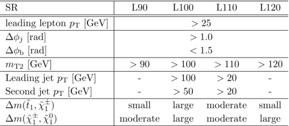
(11) steeply falling and by requiring mT2 > 40 GeV the tt̄ becomes the dominant background in the SF sample as well. χ̃0 The leptonic mT2 selection has been optimised to target models with ∆m(χ̃± 1 , 1) > m(W ) (figure 1 (a)). The jet pT spectrum is exploited in order to provide sensitivity to models with varying jet multiplicity. Four non-exclusive SRs are defined, with different selections on mT2 and on the transverse momentum of the two leading jets, as reported in table 1. The SRs L90 and L120 require mT2 > 90 GeV and mT2 > 120 GeV, respectively, with no additional requirement on jets. They provide sensitivity to scenarios with a small ∆m(t̃1 , χ̃± 1 ) (almost degenerate top squark and chargino), where the production of high-pT jets is not expected. The SR L100 has a tight jet selection, requiring at least two jets with pT > 100 GeV and pT > 50 GeV, respectively, and mT2 > 100 GeV. This SR provides sensitivity to scenarios ± χ̃0 with both large ∆m(t̃1 , χ̃± 1 ) and ∆m(χ̃1 , 1 ), where large means bigger than the W boson mass. SR L110 has a looser selection on jets, requiring two jets with pT > 20 GeV each and mT2 > 110 GeV. It provides sensitivity to scenarios with small to moderate (up to around the W boson mass) values of ∆m(t̃1 , χ̃± 1 ) resulting in moderate jet activity. Table 1. Signal regions used in the leptonic mT2 analysis. The last two rows give the relative sizes of the mass splittings that the SRs are sensitive to: small (almost degenerate), moderate (up to around the W boson mass) or large (bigger than the W boson mass).. SR leading lepton pT [GeV] ∆φj [rad] ∆φb [rad] mT2 [GeV] Leading jet pT [GeV] Second jet pT [GeV] ∆m(t̃1 , χ̃± 1) ± ∆m(χ̃1 , χ̃01 ). 5.3. L90. > 90 small moderate. L100. L110. > 25 > 1.0 < 1.5 > 100 > 110 > 100 > 20 > 50 > 20 large moderate large moderate. L120. > 120 small large. Hadronic mT2 selection. In contrast to the leptonic mT2 selection, the hadronic mT2 selection is designed to be sensitive to the models with chargino–neutralino mass differences smaller than the W mass (figure 1 (b)). In addition to the preselection described in section 5.1, events in the SR (indicated as H160) are required to satisfy the requirements given in table 2. The requirement of two b-jets favours signal over background; the targeted signal events have in general higher-pT b-jets as a result of a large ∆m(t̃1 , χ̃± 1 ) (figure 1 (b)). The tt̄ background is then further reduced by the mb−jet requirement, which preferentially selects signal models with T2. –9–.

(12) large ∆m(t̃1 , χ̃± 1 ) over the SM background. The requirement on leading lepton pT has little impact on the signal, but reduces the remaining Z/γ ∗ +jets background to a negligible level. Table 2. Signal region used in the hadronic mT2 analysis. The last two rows give the relative sizes of the mass splittings that the SR is sensitive to: small (almost degenerate), moderate (up to around the W boson mass) or large (bigger than the W boson mass).. 5.4. SR. H160. b-jets Leading lepton pT [GeV] mT2 [GeV] mb−jet [GeV] T2 ∆m(t̃1 , χ̃± 1) ± ∆m(χ̃1 , χ̃01 ). =2 < 60 < 90 > 160 large small. Multivariate analysis. In this analysis, t̃1 → t + χ̃01 signal events are separated from SM backgrounds using an MVA technique based on boosted decision trees (BDT) that uses a gradient-boosting algorithm (BDTG) [87]. In addition to the preselection described in section 5.1, events are required to have at least two jets, a leading jet with pT > 50 GeV and meff > 300 GeV. The selected events are first divided into four (non-exclusive) categories, with the requirements in each 0 category designed to target different t̃1 and χ̃1 masses: miss > 50 GeV: provides good sensitivity for m(t̃ ) in the range 200–500 GeV - (C1) ET 1 and for low neutralino masses; miss > 80 GeV: provides good sensitivity along the m(t̃ ) = m(t) + m(χ̃0 ) bound- (C2) ET 1 1 ary; miss > 50 GeV and leading lepton p > 50 GeV: provides good sensitivity for - (C3) ET T m(t̃1 ) in the range 400–500 GeV, and m(t̃1 ) > 500 GeV for high neutralino masses; miss > 50 GeV and leading lepton p > 80 GeV: provides good sensitivity for - (C4) ET T m(t̃1 ) > 500 GeV.. Events are then further divided into those containing an SF lepton pair and those containing a DF lepton pair. Categories (C1), (C2) and (C4) are considered for DF events, and categories (C1) and (C3) for SF events. A BDTG discriminant is employed to further optimise the five subcategories (three for DF, two for SF) described above. The following variables are given as input to the BDTG:. – 10 –.

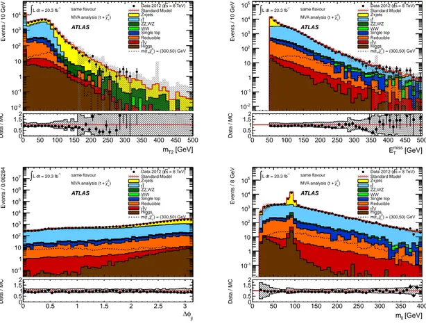
(13) ∫L dt = 20.3 fb. -1. 104. Data 2012 ( s = 8 TeV) Standard Model Z+jets tt ZZ,WZ WW Single top Reducible ttV Higgs ~ ∼0 m(t ,χ ) = (300,50) GeV. same flavour ∼) MVA analysis (t + χ 0 1. ATLAS. 103. Events / 10 GeV. Events / 10 GeV. miss , m , m , ∆φ , ∆θ , ∆φ and ∆φ . These variables are well modelled by the simulaET T2 `` `` `` l j` tion and are effective in discriminating t + χ̃01 signal from SM background; the distributions in data and MC simulation for the four “best ranked” (their correlation with the BDTG ranges from ∼ 80% to ∼ 95%) input variables for the SF and DF channels after C1 cuts are shown in figures 2 and 3, respectively. In each of the sub-figures, the uncertainty band represents the total uncertainty, from all statistical and systematic uncertainty sources (section 7). The correlation coefficient between each pair of variables is found to be in good agreement (within 1–2%) between data and MC.. 102. ∫L dt = 20.3 fb. -1. 4. Data 2012 ( s = 8 TeV) Standard Model Z+jets tt ZZ,WZ WW Single top Reducible ttV Higgs ~ ∼0 m(t ,χ ) = (300,50) GeV. same flavour ∼) MVA analysis (t + χ 0. 10. 1. ATLAS. 103 102. 1 1. 10. 1 1. 10. 1. 1. 10-1. 10-1. 10-2 20 1.5 1 0.5 0. 0. 50. 100. 150. 200. 250. 300. 350. 400. 450. 500. mT2 [GeV]. 50. 100. 150 200. 250. 300. 350. 400. 450. 500. Data / MC. Data / MC. 5. 10. 10-2 20 1.5 1 0.5 0. 0. 50. 100. 150. 200. 250. 300. 350. 400. 50. 100. 150 200. 250. 300. 350. 400. -1. Data 2012 ( s = 8 TeV) Standard Model Z+jets tt ZZ,WZ WW Single top Reducible ttV Higgs ~ ∼0 m(t ,χ ) = (300,50) GeV. same flavour 0 MVA analysis (t + ∼ χ) 1. 106. Events / 8 GeV. Events / 0.06284. ∫L dt = 20.3 fb. ATLAS. 5. 10. 104. ∫L dt = 20.3 fb. -1. 5. 10. 450. 500. Data 2012 ( s = 8 TeV) Standard Model Z+jets tt ZZ,WZ WW Single top Reducible ttV Higgs ~ ∼0 m(t ,χ ) = (300,50) GeV. same flavour 0 MVA analysis (t + ∼ χ) 1. ATLAS. 104 103. 1 1. 10. 102. 102. 10. 3. 500. Emiss [GeV] T. mT2 [GeV]. 107. 450. Emiss [GeV] T. 10. 1 1. 1. 1 10-1 20 1.5 1 0.5 0. 0. 10 0.5. 0.5. 1. 1. 1.5. 1.5. 2. 2. 2.5. 2.5. 3 ∆φ. jl. 3. Data / MC. Data / MC. -1. ∆φ. 20 1.5 1 0.5 0 0. 50. 100. 150. 200. 250. 300. 350. 400. mll [GeV]. 50. 100. 150. 200. 250. 300. 350. 400. mll [GeV]. jl. miss Figure 2. The four best ranked input variables for the MVA analysis. SF channel: mT2 , ET , ∆φj` miss and m`` after C1 cuts (ET > 50 GeV). The contributions from all SM backgrounds are shown as a histogram stack; the bands represent the total uncertainty from statistical and systematic sources. The components labelled “Reducible” correspond to the fake and non-prompt lepton backgrounds and are estimated from data as described in section 6.2; the other backgrounds are estimated from MC simulation.. Several BDTGs are trained using the simulated SM background against one or more representative signal samples, chosen appropriately for each of the five subcategories. The BDTG training parameters are chosen to best discriminate signal events from the background, with-. – 11 –.

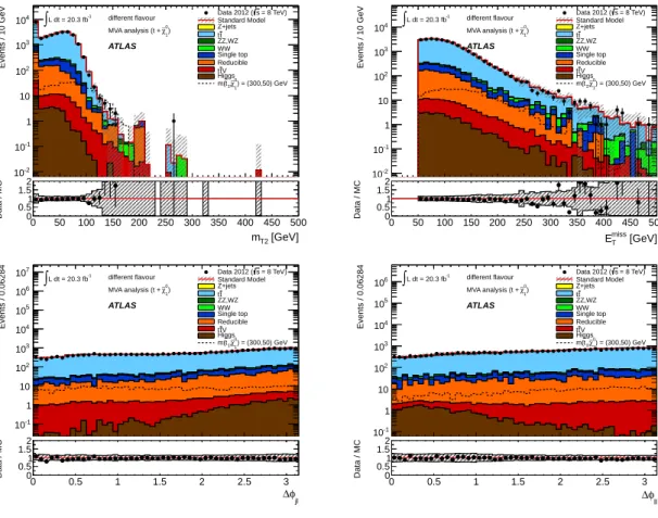
(14) ∫L dt = 20.3 fb. -1. Data 2012 ( s = 8 TeV) Standard Model Z+jets tt ZZ,WZ WW Single top Reducible ttV Higgs ~ 0 m(t ,∼ χ ) = (300,50) GeV. different flavour 0 MVA analysis (t + ∼ χ) 1. 103. Events / 10 GeV. Events / 10 GeV. 104. ATLAS. 2. 10. ∫L dt = 20.3 fb. -1. 104. Data 2012 ( s = 8 TeV) Standard Model Z+jets tt ZZ,WZ WW Single top Reducible ttV Higgs ~ 0 m(t ,∼ χ ) = (300,50) GeV. different flavour 0 MVA analysis (t + ∼ χ) 1. ATLAS. 103 102. 1 1. 1 1. 10. 10. 1. 1. -1. 10. 10-1. -2. 20 1.5 1 0.5 0 0. 50. 100. 150. 200. 250. 300. 350. 400. 450. 500. mT2 [GeV]. 50. 100. 150 200. 250. 300. 350. 400. 450. 500. Data / MC. Data / MC. 10. 10-2 20 1.5 1 0.5 0. 0. 50. 100. 150. 200. 250. 300. 350. 400. 50. 100. 150 200. 250. 300. 350. 400. ∫L dt = 20.3 fb. -1. Data 2012 ( s = 8 TeV) Standard Model Z+jets tt ZZ,WZ WW Single top Reducible ttV Higgs ~ 0 m(t ,∼ χ ) = (300,50) GeV. different flavour ∼) MVA analysis (t + χ 0 1. ATLAS. 5. 10. Events / 0.06284. Events / 0.06284. 106. 4. 10. 103. 106. 450. 500. -1. Data 2012 ( s = 8 TeV) Standard Model Z+jets tt ZZ,WZ WW Single top Reducible ttV Higgs ~ 0 m(t ,∼ χ ) = (300,50) GeV. different flavour ∼) MVA analysis (t + χ 0 1. 5. 10. ATLAS. 104. 1 1. 2. 10. 10. 10. 10. 1. 1. 10-1. -1. 10 0.5. 0.5. 1. 1. 1.5. 1.5. 2. 2. 2.5. 2.5. 3 ∆φ. jl. 3. Data / MC. Data / MC. ∫L dt = 20.3 fb. 103. 1 1. 2. 20 1.5 1 0.5 0 0. 500. Emiss [GeV] T. mT2 [GeV] 107. 450. Emiss [GeV] T. ∆φ. 20 1.5 1 0.5 0 0. 0.5. 1. 1.5. 2. 2.5. 3 ∆φ. 0.5. 1. 1.5. 2. 2.5. 3. ll. ∆φ. jl. ll. miss Figure 3. The four best ranked input variables for the MVA analysis. DF channel: mT2 , ET , ∆φj` and ∆φ`` after C1 cuts. The contributions from all SM backgrounds are shown as a histogram stack; the bands represent the total uncertainty from statistical and systematic sources. The components labelled “Reducible” correspond to the fake and non-prompt lepton backgrounds and are estimated from data as described in section 6.2; the other backgrounds are estimated from MC simulation.. out being overtrained (MC sub-samples, which are statistically independent to the training sample, are used to check that the results are reproducible). The resulting discriminants are bound between −1 and 1. The value of the cut on each of these discriminants is chosen to maximise sensitivity to the signal points considered, with the possible values of the BDTG threshold scanned in steps of 0.01. A total of nine BDTGs (five for DF events, four for SF events) and BDTG requirements are defined, setting the SRs. They are summarised in table 3.. – 12 –.

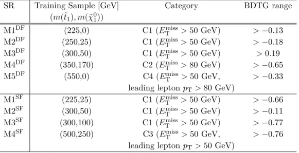
(15) Table 3. Signal regions for the MVA analysis. The first column gives the name of each SR, where DF and SF indicate different and same flavours, respectively. The second column gives the signal sample used to train the BDTG. The third column lists the selection requirements applied in addition to the BDTG requirement given in the fourth column and the common SR requirements: ≥ 2 jets, leading jet pT > 50 GeV, meff > 300 GeV.. SR. Training Sample [GeV] (m(t̃1 ), m(χ̃01 )). Category. BDTG range. M1DF M2DF M3DF M4DF M5DF. (225,0) (250,25) (300,50) (350,170) (550,0). > −0.13 > −0.18 > 0.19 > −0.65 > −0.33. M1SF M2SF M3SF M4SF. (225,25) (300,50) (300,100) (500,250). miss > 50 GeV) C1 (ET miss > 50 GeV) C1 (ET miss > 50 GeV) C1 (ET miss > 80 GeV) C2 (ET miss > 50 GeV, C4 (ET leading lepton pT > 80 GeV) miss > 50 GeV) C1 (ET miss > 50 GeV) C1 (ET miss > 50 GeV) C1 (ET miss > 50 GeV, C3 (ET leading lepton pT > 50 GeV). – 13 –. > −0.66 > −0.11 > −0.77 > −0.76.

(16) 6. Standard Model background determination. All backgrounds containing prompt leptons from W , Z or H decay are estimated directly from MC simulation. The dominant backgrounds (top-quark pair production for all analyses, and diboson and W t single-top production for the leptonic mT2 and hadronic mT2 analyses respectively) are normalised to data in dedicated CRs, and then extrapolated to the SRs using the MC simulation (with a likelihood fit as described in section 6.1). Whilst it is not a dominant background, Z/γ ∗ +jets is also normalised in a dedicated CR in the hadronic mT2 analysis. All other such contributions are normalised to their theoretical cross-sections. The backgrounds due to non-prompt leptons (from heavy-flavour decays or photon conversions) or jets misidentified as leptons are estimated using a data-driven technique. Events with these types of lepton are referred to as “fake and non-prompt” lepton events. The estimation procedure is common to all three analyses and is described in section 6.2. 6.1. Background fit. The observed numbers of events in the CRs are used to derive SM background estimates in each SR via a profile likelihood fit [88]. This procedure takes into account the correlations across the CRs due to common systematic uncertainties and the cross-contamination in each CR from other SM processes. The fit takes as input, for each SR: 1. The number of events observed in each CR and the corresponding number of events predicted in each by the MC simulation for each (non-fake, prompt) background source. 2. The number of events predicted by the MC simulation for each (non-fake, prompt) background source. 3. The number of fake and non-prompt lepton events in each region (CRs and SR) obtained with the data-driven technique (see section 6.2). Each uncertainty source, as detailed in section 7, is treated as a nuisance parameter in the fit, constrained with a Gaussian function taking into account the correlations between sample estimates. The likelihood function is the product of Poisson probability functions describing the observed and expected number of events in the control regions and the Gaussian constraints on the nuisance parameters. For each analysis, and each SR, the free parameters of the fit are the overall normalisations of the CR-constrained backgrounds: tt̄, W W and (W Z, ZZ) for the leptonic mT2 analysis; tt̄, W t and Z/γ ∗ +jets for the hadronic mT2 analysis and tt̄ for the MVA analysis. The contributions from all other non-constrained prompt-lepton processes are set to the MC expectation, but are allowed to vary within their respective uncertainties. The contribution from fake and non-prompt lepton events is also set to its estimated yield and allowed to vary within its uncertainty. The fitting procedure maximises this likelihood by adjusting the free parameters; the fit constrains only the background normalisations, while the systematic uncertainties are left unchanged (i.e. the nuisance parameters always have a. – 14 –.

(17) central value very close to zero with an error close to one). Background fit results are crosschecked in validation regions (VRs) located between, and orthogonal to, the control and signal regions. Sections 6.3 to 6.5 describe the CR defined for each analysis and, in addition, any VRs defined to cross-check the background fit results. 6.2. Fake and non-prompt lepton background estimation. The fake and non-prompt lepton background arises from semi-leptonic tt̄, s-channel and t-channel single-top, W +jets and light- and heavy-flavour jet production. The main contributing source in a given region depends on the topology of the events: low-mT2 regions are expected to be dominated by the multijet background, while regions with moderate/high mT2 are expected to be dominated by the W +jets and tt̄ production. The fake and non-prompt lepton background rate is estimated for each analysis from data using a matrix method estimation, similar to that described in refs. [89, 90]. In order to use the matrix method, two types of lepton identification criteria are defined: tight, corresponding to the full set of identification criteria described above, and loose, corresponding to preselected electrons and muons. The number of events containing fake leptons in each region is obtained by acting on a vector of observed (loose, tight) counts with a 4 × 4 matrix with terms containing probabilities (f and r) that relate real–real, real–fake, fake–real and fake–fake lepton event counts to tight–tight, tight–loose, loose–tight and loose–loose counts. The two probabilities used in the prediction are defined as follows: r is the probability for real leptons satisfying the loose selection criteria to also pass the tight selection and f is the equivalent probability for fake and non-prompt leptons. The probability r is measured using a Z → ``(` = e, µ) sample, while the probability f is measured from two background-enriched control samples. The first of these requires exactly one lepton with pT > 25 GeV, at least miss < 25 GeV, and an angular distance ∆R < 0.5 between the leading jet and the one jet, ET lepton, in order to enhance the contribution from the multijet background. The probability is parameterised as a function of the lepton η and pT and the number of jets. For leptons with pT < 25 GeV, in order to avoid trigger biases, a second control sample which selects events containing a same-charge DF lepton pair is used. The probability f is parameterised as a function of lepton pT and η, the number of jets, meff and mT2 . The last two variables help to isolate the contributions expected to dominate from multijet, W +jets or tt̄ productions. In both control samples, the probability is parameterised by the number of b-jets when a b-jet is explicitly required in the event selection (i.e. in the hadronic mT2 ), in order to enhance the contribution from heavy-flavour jet production. Many sources of systematic uncertainty are considered when evaluating this background. Like the probabilities themselves, the systematic uncertainties are also parameterised as a function of the lepton and event variables discussed above. The parameterised uncertainties are in general dominated by differences in the measurement of the fake lepton probabilities obtained when using the two control regions above. The limited number of events in the CR used to measure the probabilities are also considered as a source of systematic uncertainty. The overall systematic uncertainty ranges between 10% and 50% across the various regions. – 15 –.

(18) (control, validation and signal). Ultimately, in SRs with very low predicted event yields the overall uncertainty on the fake and non-prompt lepton background yield is dominated by the statistical uncertainty arising from the limited number of data events in the SRs, which reaches 60–80% in the less populated SRs. In these regions, however, the contributions from fake and non-prompt lepton events are small or negligible. The predictions obtained using this method are validated in events with same-charge lepton pairs. As an example, figure 4 shows the distribution of meff and mT2 in events with a same-charge lepton pair after the preselection described in section 5.1, prior to any additional selection. 6.3. Leptonic mT2 analysis. The dominant SM background contributions in the SRs are tt̄ and W W decays. Other diboson processes also expected to contribute significantly are: W Z in its 3-lepton decay mode and ZZ decaying to two leptons and two neutrinos. A single dedicated CR is defined for each of these backgrounds (CRXL , where X=T,W,Z for the tt̄, W W and other diboson productions respectively). Predictions in all SRs make use of the three common CRs. This choice was optimised considering the background purity and the available sample size. The validity of the combined background estimate is tested using a set of four validation regions (VRX L , where X describes the specific selection under validation). The definitions of the CRs and VRs are given in table 4. The validity of the tt̄ background prediction for 110 different jet selections is checked in VR100 L and VRL . miss (Higgs, W t, Z/γ ∗ → Additional SM processes yielding two isolated leptons and large ET ``+jets and tt̄V ) and providing a sub-dominant contribution to the SRs are determined from MC simulation. The fake and non-prompt lepton background is a small contribution (less than 10% of the total background). The composition before and after the likelihood fit is given in table 5 for the CRs and table 6 for the VRs. In these (and all subsequent) composition tables the quoted uncertainty includes all the sources of statistical and systematic uncertainty considered (see section 7.). The purity of the CRs is improved by exploiting flavour information and selecting either DF or SF pairs depending on the process being considered. The normalisation factors derived are, however, applied to all the events in a given process (both DF and SF). Checks were performed to demonstrate that the normalisation factors are not flavour-dependent. Good agreement is found between data and the SM prediction before and after the fit, leading to normalisation factors compatible with unity. The normalisations of the tt̄, W W and W Z, ZZ backgrounds as obtained from the fit are 0.91 ± 0.07, 1.27 ± 0.24 and 0.85 ± 0.16 respectively. The number of expected signal events in the CRs was investigated for each signal model considered. The signal contamination in CRTL and CRWL is negligible, with the exception of signal models with top squark masses close to the top-quark mass. In this case, the signal contamination can be as high as 20% in CRTL and up to 100% in CRWL . The signal contamination in CRZL is typically less than 10%, with a few exceptions; for signal models with top-squark masses below 250 GeV, the contamination is closer to 30%, and for signal. – 16 –.

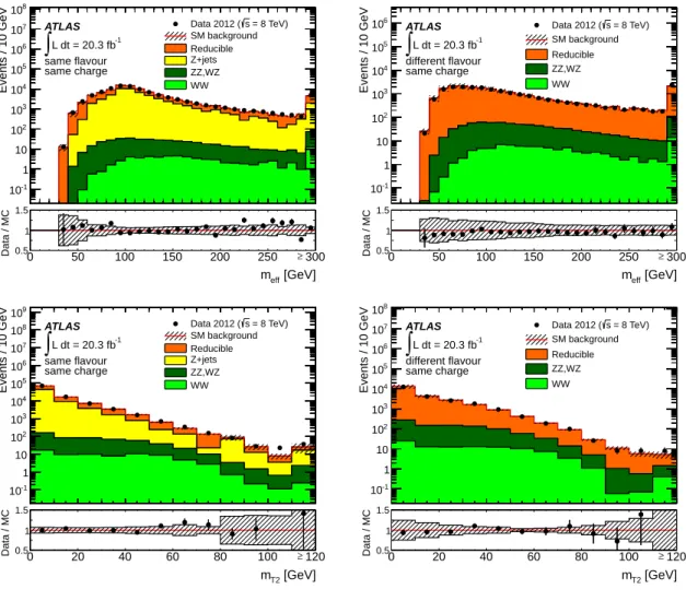
(19) Data 2012 ( s = 8 TeV) SM background Reducible Z+jets ZZ,WZ WW. ATLAS. 107. ∫. -1. L dt = 20.3 fb same flavour same charge. 6. 10. 105. Events / 10 GeV. Events / 10 GeV. 108. 104. 106. ATLAS. 105. L dt = 20.3 fb different flavour same charge. ∫. 104. Data 2012 ( s = 8 TeV) SM background. -1. Reducible ZZ,WZ WW. 103. 3. 10. 102. 102. 10. 10. 1. 1. -1. 10. 1.5 1 0.5. 0. 50. 100. 150. 200. 250. ≥ 300. Data / MC. Data / MC. 10-1. 1.5 1 0.5. 0. 50. 100. 150. 200. 109 10. ATLAS. 107. L dt = 20.3 fb same flavour same charge. 8. ∫. 106. Data 2012 ( s = 8 TeV) SM background Reducible Z+jets ZZ,WZ WW. -1. 105 104. ≥ 300. 108 Data 2012 ( s = 8 TeV) SM background. ATLAS. 107. ∫. -1. L dt = 20.3 fb different flavour same charge. 6. 10. 105. Reducible ZZ,WZ WW. 104 3. 10. 103. 102. 2. 10. 10. 10. 1. 10-1. 10-1. 1.5. 1.5. 1 0.5. 0. 20. 40. 60. 80. 100. ≥ 120. mT2 [GeV]. Data / MC. 1. Data / MC. 250. meff [GeV] Events / 10 GeV. Events / 10 GeV. meff [GeV]. 1 0.5. 0. 20. 40. 60. 80. 100. ≥ 120. mT2 [GeV]. Figure 4. Distributions of meff (top) and mT2 (bottom), for SF (left) and DF (right) same-charge lepton pairs, after the preselection requirements described in section 5.1. The components labelled “Reducible” correspond to the fake and non-prompt lepton backgrounds and are estimated from data as described in section 6.2. The other SM backgrounds processes which are expected to contribute events with two real leptons are shown and are estimated from MC simulation. The reconstructed leptons are required to match with a generator-level lepton in order to avoid any double counting of the total fake and non-prompt lepton contribution. The bands represent the total uncertainty.. models with small ∆m(t̃1 , χ̃± 1 ) the signal contamination is as high as 100%. The same CRs can be kept also for these signal models, despite the high signal contamination, since the expected yields in the SRs would be large enough for these signal models to be excluded even in the hypothesis of null expected background. The signal contamination in the VRs can be up to ∼ 100% for signal models with top-quark-like kinematics and becomes negligible when considering models with increasing top-squark masses. Figure 5 (top) shows the p`` Tb distribution for DF events with 40 < mT2 < 80 GeV,. – 17 –.

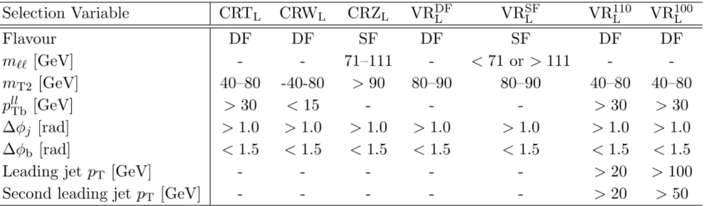
(20) Table 4. Definitions of the CRs and VRs in the leptonic mT2 analysis: CRTL (used to constrain tt̄), CRWL (used to constrain W W ), CRZL (used to constrain W Z and ZZ), VRDF L (validation region for 110 DF), VRSF (validation region for SF), VR (validation region for L110 jet requirements) and VR100 L L L (validation region for L100 jet requirements).. Selection Variable. CRTL. CRWL. CRZL. VRDF L. VRSF L. VR110 L. VR100 L. Flavour m`` [GeV] mT2 [GeV] pllTb [GeV] ∆φj [rad] ∆φb [rad] Leading jet pT [GeV] Second leading jet pT [GeV]. DF 40–80 > 30 > 1.0 < 1.5 -. DF -40-80 < 15 > 1.0 < 1.5 -. SF 71–111 > 90 > 1.0 < 1.5 -. DF 80–90 > 1.0 < 1.5 -. SF < 71 or > 111 80–90 > 1.0 < 1.5 -. DF 40–80 > 30 > 1.0 < 1.5 > 20 > 20. DF 40–80 > 30 > 1.0 < 1.5 > 100 > 50. ∆φ > 1.0 and ∆φb < 1.5. The range p`` Tb < 15 GeV corresponds to the CRWL while the `` events with pTb > 30 GeV are those entering in CRTL . Figure 5 (bottom) shows the mT2 distribution for SF events with ∆φ > 1.0 and ∆φb < 1.5 and m`` within 20 GeV of the Z boson mass. The events with mT2 > 90 GeV in this figure are those entering CRZL .. – 18 –.

(21) Table 5. Background fit results for the three CRs in the leptonic mT2 analysis. The nominal expectations from MC simulation are given for comparison for those backgrounds (tt̄, W W , W Z and ZZ) which are normalised to data. Combined statistical and systematic uncertainties are given. Events with fake or non-prompt leptons are estimated with the data-driven technique described in section 6.2. The observed events and the total (constrained) background are the same by construction. Entries marked - - indicate a negligible background contribution. Uncertainties on the predicted background event yields are quoted as symmetric except where the negative error reaches down to zero predicted events, in which case the negative error is truncated. Channel. CRTL. CRWL. CRZL. Observed events. 12158. 913. 174. 12158 ± 110. 913 ± 30. 174 ± 13. 8600 ± 400 1600 ± 400 64 ± 14. 136 ± 24 630 ± 50 14 ± 5. 27 ± 6 14 ± 4 112 ± 19. 12700 ± 700. 800 ± 90. 190 ± 20. 9500 ± 600 1260 ± 110 76 ± 12 9+11 −9 10.8 ± 3.4 1070 ± 90 67 ± 21 740 ± 90. 150 ± 25 490 ± 80 17 ± 4 1.5+2.2 −1.5 0.08 ± 0.04 35 ± 7 20 ± 6 81 ± 16. 30 ± 7 10.7 ± 2.5 132 ± 11 19 ± 8 0.64 ± 0.21 1.6 ± 1.1 0.08 ± 0.04 --. Total (constrained) bkg events Fit output, tt̄ events Fit output, W W events Fit output, W Z, ZZ events Total expected bkg events Fit input, expected tt̄ events Fit input, expected W W events Fit input, expected W Z, ZZ events Expected Z/γ ∗ → `` events Expected tt̄ V events Expected W t events Expected Higgs boson events Expected events with fake and non-prompt leptons. – 19 –.

(22) Table 6. Background fit results for the four VRs in the leptonic mT2 analysis. Combined statistical and systematic uncertainties are given. Events with fake or non-prompt leptons are estimated with the data-driven technique described in section 6.2. The observed events and the total (constrained) background are the same in the CRs by construction; this is not the case for the VRs, where the consistency between these event yields is the test of the background model. Entries marked - indicate a negligible background contribution. Uncertainties on the predicted background event yields are quoted as symmetric except where the negative error reaches down to zero predicted events, in which case the negative error is truncated. VRSF L. VRDF L. VR110 L. VR100 L. Observed events. 494. 622. 8162. 1370. Total bkg events. 500 ± 40. Channel. 620 ± 50 7800 ± 400 1390 ± 110. Fit output, tt̄ events 338 ± 19 430 ± 29 6800 ± 400 1230 ± 110 Fit output, W W events 97 ± 22 121 ± 27 290 ± 70 38 ± 15 Fit output, W Z, ZZ events 5.8 ± 1.1 2.2 ± 1.4 13.5 ± 3.2 1.5 ± 1.2 Expected Z/γ ∗ → `` events 4+5 -3+5 1+1 −4 −3 −1 Expected tt̄ V events 0.48 ± 0.18 0.80 ± 0.27 10.1 ± 3.1 4.1 ± 1.3 Expected W t events 39 ± 8 60 ± 10 430 ± 50 62 ± 8 Expected Higgs boson events 0.39 ± 0.16 0.55 ± 0.20 14 ± 4 1.7 ± 0.6 Expected events with fake and non-prompt leptons 10.5 ± 3.5 13 ± 4 275 ± 33 45 ± 7. – 20 –.

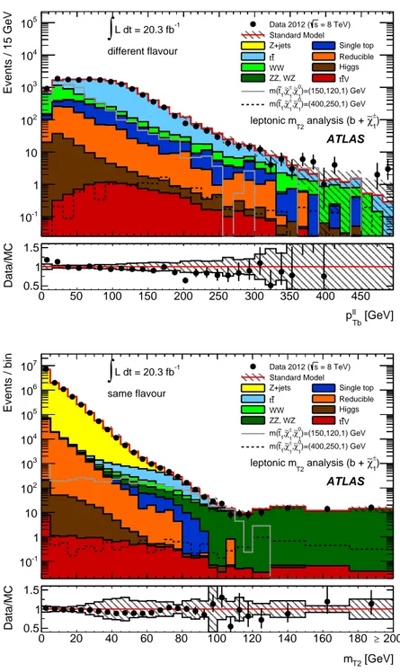
(23) Events / 15 GeV. 10. ∫ L dt = 20.3 fb. 104. different flavour. 5. Data 2012 ( s = 8 TeV) Standard Model Z+jets Single top Reducible tt Higgs WW ZZ, WZ ttV ~ ± ∼0 m(t ,∼ χ ,χ )=(150,120,1) GeV. -1. 3. 10. 1 1. 1. ~ ± ∼0 m(t1,∼ χ ,χ )=(400,250,1) GeV 1. 102. 1. leptonic m. T2. analysis (b + ∼ χ1) ±. ATLAS 10 1. Data/MC. 10-1. 1.50. 50. 100. 150. 200. 250. 300. 350. 400. 1 0.5 0. 450 pll [GeV] Tb. 50. 100. 150. 200. 250. 300. 350. 400. 450 pll [GeV]. Events / bin. Tb. ∫ L dt = 20.3 fb. 107 6. 10. Data 2012 ( s = 8 TeV) Standard Model Z+jets Single top Reducible tt Higgs WW ZZ, WZ ttV ~ ∼± ∼0 m(t ,χ ,χ )=(150,120,1) GeV. -1. same flavour. 5. 10. 104. 1 1. 1. 1. 1. ~ ± ∼0 m(t1,∼ χ ,χ )=(400,250,1) GeV. 3. leptonic m. 10. T2. analysis (b + ∼ χ1) ±. ATLAS. 102 10 1 -1. Data/MC. 10. 1.50. 20. 40. 60. 80. 100. 120. 140. 160. 200. mT2 [GeV]. 1 0.5 0. 180. 20. 40. 60. 80. 100. 120. 140. 160. 180 ≥ 200 mT2 [GeV]. Figure 5. Top: distribution of p`` Tb for DF events with 40 < mT2 < 80 GeV, ∆φj > 1.0 rad and ∆φb < 1.5 rad. Bottom: Distribution of mT2 for SF events with a dilepton invariant mass in the 71–111 GeV range, ∆φ > 1.0 rad and ∆φb < 1.5 rad. The contributions from all SM backgrounds are shown as a histogram stack; the bands represent the total uncertainty. The components labelled “Reducible” correspond to the fake and non-prompt lepton backgrounds and are estimated from data as described in section 6.2; the other backgrounds are estimated from MC simulation. The expected distribution for two signal models is also shown. The full line corresponds to a model 0 with m(t̃1 ) = 150 GeV, m(χ̃± 1 ) = 120 GeV and m(χ̃1 ) = 1 GeV; the dashed line to a model with ± 0 m(t̃1 ) = 400 GeV, m(χ̃1 ) = 250 GeV and m(χ̃1 ) = 1 GeV.. – 21 –.

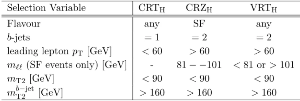
(24) 6.4. Hadronic mT2 analysis. Top-quark pair and single-top (W t-Channel) production contribute significantly to the background event yields in the SR for this analysis. Simulation shows that 49% of background events in the SR are from top-quark pair production and 37% are from W t. The next most significant SM background contributions are those arising from fake or non-prompt leptons. The remainder of the background is composed of Z/γ ∗ +jets and W W events. The contributions from other diboson (W Z and ZZ), tt̄V and Higgs processes are negligible, and are estimated using the MC simulation. The CRs are defined for the combined tt̄ and W t process, and Z/γ ∗ (→ ee, µµ)+jets backgrounds (the Z/γ ∗ (→ τ τ )+jets contribution is fixed at the MC expectation). The contribution from W t in the SR is dominated by its NLO contributions (which can be interpreted as top-pair production, followed by decay of one of the top-quarks). These CRs are referred to as CRXH , where X=T,Z for the (tt̄, W t) and Z/γ ∗ (→ ee, µµ)+jet backgrounds respectively. The validity of the combined estimate of the W t and tt̄ backgrounds is tested using a validation region for the top-quark background (VRTH ). The definitions of these regions are given in table 7, and their composition before and after the likelihood fit described in section 6.1 is given in table 8. Good agreement is found between data and SM prediction before and after the fit, leading to normalisations consistent with one: 0.93 ± 0.32 for the (tt̄,W t) and 1.5 ± 0.5 for the Z/γ ∗ +jets backgrounds. The signal contamination in CRZH is negligible, whilst in CRTH it is of order 10% (16%) for models with a 300 GeV top squark and a 150 GeV (100 GeV) chargino, for neutralino masses below 100 GeV, which the region where H160 is sensitive. The signal contamination in VRTH is much higher (∼ 30%) in the same mass-space. Table 7. Definitions of the CRs and VR in the hadronic mT2 analysis: CRTH (used to constrain tt̄ and W t), CRZH (used to constrain Z/γ ∗ +jets decays to ee and µµ) and VRTH (validation region for tt̄ and W t).. Selection Variable. CRTH. CRZH. VRTH. Flavour b-jets leading lepton pT [GeV] m`` (SF events only) [GeV] mT2 [GeV] b−jet mT2 [GeV]. any =1 < 60 < 90 > 160. SF =2 > 60 81 − −101 < 90 > 160. any =2 > 60 < 81 or > 101 < 90 > 160. Figure 6 shows the mb−jet distribution for events with one b-jet (using the highest pT jet T2 which is not a b-jet with the single b-jet in the calculation of mb−jet T2 ), mT2 < 90 GeV and b-jet leading lepton pT < 60 GeV. The events with mT2 > 160 GeV in the figure are those entering CRTH . The data are in agreement with the background expectation across the distribution.. – 22 –.

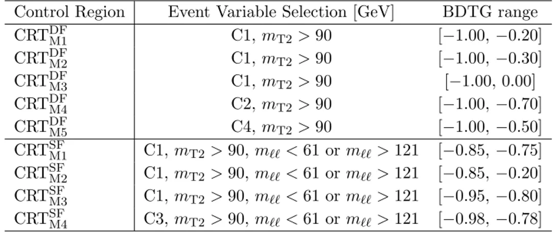
(25) Table 8. Background fit results for the two CRs and VR region in the hadronic mT2 analysis. The nominal expectations from MC simulation are given for comparison for those backgrounds (tt̄, W t and Z/γ ∗ (→ ee, µ+ µ− )+jets production) which are normalised to data. Combined statistical and systematic uncertainties are given. Events with fake or non-prompt leptons are estimated with the data-driven technique described in section 6.2. The observed events and the total (constrained) background are the same in the CRs by construction; this is not the case for the VR, where the consistency between these event yields is the test of the background model. Uncertainties on the predicted background event yields are quoted as symmetric except where the negative error reaches down to zero predicted events, in which case the negative error is truncated. Channel. CRTH. CRZH. VRTH. 315. 156. 112. Total (constrained) bkg events. 315 ± 18. 156 ± 13. 110 ± 50. Fit output, tt̄, W t events Fit output, Z/γ ∗ → ee, µµ+jets events. 256 ± 27 0.9+1.1 −0.9. 4±4 147 ± 13. 70 ± 40 20 ± 8. Total expected bkg events. 335 ± 90. 110 ± 36. 110 ± 60. 280 ± 90 0.6+0.7 −0.6 3+4 −3 2.3 ± 0.8 0.40 ± 0.16 23 ± 17 29.4 ± 1.7 0.35 ± 0.05. 5±5 100 ± 34 0.07+0.14 −0.07 1.5 ± 0.5 0.06+0.32 −0.06 0.14 ± 0.09 0.36 ± 0.24 2.06 ± 0.30. 80 ± 60 13.8 ± 2.4 1+3 −1 2.3 ± 0.7 0.10+0.15 −0.10 2.15 ± 0.28 12.8 ± 1.2 0.50 ± 0.06. Observed events. Fit input, expected tt̄, W t events Fit input, expected Z/γ ∗ → ee, µµ+jets events Expected W W events Expected tt̄V events Expected W Z, ZZ events Expected Z/γ ∗ → τ τ +jets events Expected events with fake and non-prompt leptons Expected Higgs boson events. 6.5. Multivariate analysis. In this analysis, the dominant SM background processes are top-quark pair production and diboson production. The Z/γ ∗ +jets contribution, relevant only for the SF channel, is strongly suppressed by the BDTG requirement. The CRs are defined for tt̄ (table 9) in regions mutually exclusive to the SRs, using BDTG intervals much more populated with tt̄ events, while all other SM background with two isolated leptons are small and evaluated using MC simulation. The fake and non-prompt lepton background is estimated using the method described in section 6.2. In addition to the application of all non-BDTG SR cuts, the following selections are applied in the CRs: mT2 > 90 GeV and, in SF events, m`` which must be less than 61 GeV or greater than 121 GeV. The composition before and after the likelihood fit is given in tables 10 and 11 for the DF and SF CRs, respectively. The corresponding CR for the DF DF(SF) (SF) SR labelled N is denoted CRTMN . The normalisation factors derived in each CR for tt̄ are consistent within one standard deviation (1σ) of the normalisation factor derived for tt̄ in the leptonic-mT2 analysis.. – 23 –.

(26) Entries / 10 GeV. 8. 10. 107 6. 10. Data 2012 ( s = 8 TeV) Standard Model Z+jets. ATLAS. ∫ L dt = 20.3 fb. -1. ∼) hadronic mT2 analysis (b + χ ±. 1. b-jet. [CRTH, prior to mT2 cut]. 5. 10. 104 3. tt, Wt Reducible ttV ZZ,WZ WW Higgs ~ ± ∼0 m(t1,∼ χ ,χ ) = (300,150,100) GeV ~ ±1 ∼01 m(t1,∼ χ ,χ ) = (300,100,50) GeV ~ ∼±1 ∼01 m(t1,χ ,χ ) = (300,100,1) GeV 1. 10. 1. 102 10 1. Data / MC. 10-1. 20 1.5 1 0.5 0 0. 50. 100. 150. 200. 250. 300. 350. 400. 50. 100. 150. 200. 250. 300. 350 >400 400 mb-jet T2 [GeV]. b−jet Figure 6. Distribution of mb−jet for events with 1 b-jet and all other CRTH cuts, except that on mT2 T2 itself. The contributions from all SM backgrounds are shown as a histogram stack; the bands represent the total uncertainty. The component labelled “Reducible” corresponds to the fake and non-prompt lepton background and is estimated from data as described in section 6.2; the other backgrounds are estimated from MC samples normalised to the luminosity of the data and their respective crosssections. The expected distribution for three signal models is also shown. The dotted line corresponds 0 to a model with m(t̃1 ) = 300 GeV, m(χ̃± 1 ) = 150 GeV and m(χ̃1 ) = 100 GeV; the full line corresponds ± to a model with m(t̃1 ) = 300 GeV, m(χ̃1 ) = 100 GeV and m(χ̃01 ) = 50 GeV; the dashed line to a 0 model with m(t̃1 ) = 300 GeV, m(χ̃± 1 ) = 100 GeV and m(χ̃1 ) = 1 GeV. The last bin includes the histogram overflow.. Figure 7 shows the BDTG distributions for data and MC simulation in CRTDF M3 and SF CRTM2 . The data are in agreement with the background expectations. The expected distribution for the signal point which was used to train the corresponding SR is also shown on each plot m(t̃1 ), m(χ̃01 ) = (300, 50) GeV. The validity of the background estimate is tested using a set of VRs. Analogously to the DF(SF) CR, the corresponding VR for the DF (SF) SR labelled N is referred to as VRTMN . The definitions of these regions are given in table 12 and their composition before and after the likelihood fit is given in tables 13 and 14 for the DF and SF VRs, respectively. The signal contamination in the CRs ranges from 1.5–30% (4.8–24%) in the DF (SF) CRs, whilst the contamination in the DF (SF) VRs ranges from 0.4–20% (0.9–13%).. – 24 –.

(27) Table 9. Definitions of the CRs for the MVA analysis: the name of each CR is given in the first column and these have a one-to-one correspondence with the equivalently named SR. The middle column lists all selection cuts made, whilst the final column gives the BDTG range.. Control Region CRTDF M1 CRTDF M2 CRTDF M3 CRTDF M4 CRTDF M5 CRTSF M1 CRTSF M2 CRTSF M3 CRTSF M4. Event Variable Selection [GeV] C1, mT2 > 90 C1, mT2 > 90 C1, mT2 > 90 C2, mT2 > 90 C4, mT2 > 90 C1, mT2 > 90, m`` < 61 or m`` > 121 C1, mT2 > 90, m`` < 61 or m`` > 121 C1, mT2 > 90, m`` < 61 or m`` > 121 C3, mT2 > 90, m`` < 61 or m`` > 121. BDTG range [−1.00, −0.20] [−1.00, −0.30] [−1.00, 0.00] [−1.00, −0.70] [−1.00, −0.50] [−0.85, −0.75] [−0.85, −0.20] [−0.95, −0.80] [−0.98, −0.78]. Table 10. Background fit results for the DF CRs in the MVA analysis. The nominal expectations from MC simulation are given for comparison for tt̄, which is normalised to data by the fit. Combined statistical and systematic uncertainties are given. Events with fake or non-prompt leptons are estimated with the data-driven technique described in section 6.2. The observed events and the total (constrained) background are the same in the CRs by construction. Uncertainties on the predicted background event yields are quoted as symmetric except where the negative error reaches down to zero predicted events, in which case the negative error is truncated. CRTDF M1. CRTDF M2. CRTDF M3. CRTDF M4. CRTDF M5. 419. 410. 428. 368. 251. Total (constrained) bkg events. 419 ± 20. 410 ± 20. 428 ± 21. 368 ± 19. 251 ± 16. Fit output, tt̄ events. 369 ± 23. 363 ± 23. 379 ± 24. 325 ± 22. 214 ± 19. Total expected bkg events. 430 ± 70. 420 ± 60. 440 ± 70. 380 ± 60. 260 ± 50. 380 ± 60 2.7 ± 0.8 20 ± 5 8+9 −8 1.0 ± 1.0 0.3+0.4 −0.3 0.26 ± 0.10 18 ± 4. 375± 60 2.2 ± 0.7 19 ± 5 7+8 −7 0.9+1.0 −0.9 0.31+0.35 −0.31 0.24 ± 0.10 18 ± 4. 390 ± 70 2.4 ± 0.7 20 ± 5 7+9 −7 1.0 ± 1.0 0.31+0.35 −0.31 0.26 ± 0.10 19 ± 4. 340 ± 50 2.7 ± 0.8 16 ± 5 6+8 −6 0.5+0.8 −0.5 0.3+0.4 −0.3 0.12 ± 0.05 17 ± 4. 220 ± 40 1.9 ± 0.6 15 ± 4 6+7 −6 1.0 ± 0.8 0.3+0.4 −0.3 0.19 ± 0.10 12.5 ± 3.2. Channel Observed events. Fit input, expected tt̄ Expected tt̄V events Expected W t events Expected W W events Expected ZW, ZZ events Expected Z/γ ∗ → ``+jets events Expected Higgs boson events Expected events with fake and non-prompt leptons. – 25 –.

(28) Events / 0.05. 104. ∫L dt = 20.3 fb. -1. 3. 10. Data 2012 ( s = 8 TeV) Standard Model Z+jets tt ZZ,WZ WW Single top Reducible ttV Higgs ~ 0 m(t1,∼ χ ) = (300,50) GeV. different flavour ∼) MVA analysis (t + χ 0 1. CRTDF M3. ATLAS. 102. 1. 10 1. Events / 0.05. Data / MC. 10-1 10-2 2-1 1.5 1 0.5 0 -1. -0.8. -0.6. -0.2. 0. 0.2. BDTG classifier response. -0.8. -0.6. ∫L dt = 20.3 fb. -1. 3. -0.4. 10. -0.4. -0.2 0 0.2 BDTG classifier response. Data 2012 ( s = 8 TeV) Standard Model Z+jets tt ZZ,WZ WW Single top Reducible ttV Higgs ~ 0 m(t1,∼ χ ) = (300,50) GeV. same flavour 0 MVA analysis (t + ∼ χ) 1. SF. CRTM2. 102. ATLAS. 1. 10 1. Data / MC. 10-1 10-2 2-1 1.5 1 0.5 0 -1. -0.9. -0.8. -0.7. -0.6. -0.5. -0.4. -0.3. -0.2. -0.1. 0. BDTG classifier response. -0.9. -0.8. -0.7. -0.6. -0.5. -0.4. -0.3 -0.2 -0.1 0 BDTG classifier response. SF Figure 7. BDTG distributions of data and MC events in control regions CRTDF M3 (top) and CRTM2 (bottom). The contributions from all SM backgrounds are shown as a histogram stack. The bands represent the total uncertainty. The components labelled “Reducible” correspond to the fake and nonprompt lepton backgrounds and are estimated from data as described in section 6.2; the remaining backgrounds are estimated from MC samples normalised to the luminosity of the data. The expected distribution for the signal point which was used to train the corresponding SR is also shown on each plot (see text).. – 26 –.

(29) Table 11. Background fit results for the SF CRs in the MVA analysis. The nominal expectations from MC simulation are given for comparison for tt̄, which is normalised to data by the fit. Combined statistical and systematic uncertainties are given. Events with fake or non-prompt leptons are estimated with the data-driven technique described in section 6.2. The observed events and the total (constrained) background are the same in the CRs by construction. Uncertainties on the predicted background event yields are quoted as symmetric except where the negative error reaches down to zero predicted events, in which case the negative error is truncated. CRTSF M1. CRTSF M2. CRTSF M3. CRTSF M4. 99. 79. 133. 27. Total (constrained) bkg events. 99 ± 10. 79 ± 9. 133 ± 12. 27 ± 5. Fit output, tt̄ events. 82 ± 12. 55 ± 14. 101 ± 16. 14 ± 8. Total expected bkg events. 94 ± 16. 88 ± 16. 129 ± 23. 32 ± 10. Channel Observed events. Fit input, expected tt̄ 77 ± 13 65 ± 9 95 ± 20 19 ± 7 Expected tt̄V events 0.98 ± 0.31 0.95 ± 0.31 1.4 ± 0.4 0.70 ± 0.23 +0.33 Expected W t events 1.6 ± 1.5 2.8 ± 1.6 4.0 ± 1.6 0.20−0.20 +1.7 +1.5 +1.8 +1.0 Expected W W events 1.3−1.3 1.4−1.4 1.7−1.7 0.7−0.7 Expected ZW, ZZ events 1.3 ± 0.8 2.1 ± 0.7 2.1 ± 1.3 1.4 ± 0.5 Expected Z/γ ∗ → ``+jets events 7±7 12 ± 11 14 ± 9 7±6 Expected Higgs boson events 0.06 ± 0.06 0.08 ± 0.05 0.12 ± 0.05 0.04 ± 0.04 Expected events with fake and non-prompt leptons 3.7 ± 1.7 3.7 ± 1.7 6.9 ± 2.3 2.8 ± 1.2. Table 12. VRs for the MVA analysis. The name of each VR is given in the first column and these have a one-to-one correspondence with the equivalently named SR. The middle column lists all selection cuts made, whilst the final column gives the BDTG range.. Validation Region VRTDF M1 VRTDF M2 VRTDF M3 VRTDF M4 VRTDF M5 VRTSF M1 VRTSF M2 VRTSF M3 VRTSF M4. C1, C1, C1, C3,. Event Variable Selection [GeV] C1, 80 < mT2 < 90 C1, 80 < mT2 < 90 C1, 80 < mT2 < 90 C2, 80 < mT2 < 90 C4, 80 < mT2 < 90 80 < mT2 < 90, m`` < 61 or m`` > 121 80 < mT2 < 90, m`` < 61 or m`` > 121 80 < mT2 < 90, m`` < 61 or m`` > 121 80 < mT2 < 90, m`` < 61 or m`` > 121. – 27 –. BDTG range [−0.75, −0.13] [−0.75, −0.18] [−0.80, 0.19] [−0.98, −0.65] [−0.998, −0.33] [−0.80, −0.66] [−0.85, −0.11] [−0.95, −0.77] [−0.995, −0.76].

(30) Table 13. Background fit results for the DF VRs in the MVA analysis. The nominal expectations from MC simulation are given for comparison for tt̄, which is normalised to data. Combined statistical and systematic uncertainties are given. Events with fake or non-prompt leptons are estimated with the data-driven technique described in section 6.2. The observed events and the total (constrained) background are the same in the CRs by construction; this is not the case for the VRs, where the consistency between these event yields is the test of the background model. Entries marked - indicate a negligible background contribution. Backgrounds which contribute negligibly to all VRs are not listed. Uncertainties on the predicted background event yields are quoted as symmetric except where the negative error reaches down to zero predicted events, in which case the negative error is truncated. VRTDF M1. VRTDF M2. VRTDF M3. VRTDF M4. VRTDF M5. Observed events. 149. 57. 30. 40. 47. Total bkg events. 144 ± 24. 59 ± 8. 30 ± 6. 43 ± 9. 41 ± 10. Fit output, tt̄ events. 136 ± 23. 54 ± 7. 30 ± 6. 37 ± 9. 36 ± 9. 141 ± 20 0.64 ± 0.21 4.4 ± 2.2 1.0+1.6 −1.0 0.09+0.16 −0.09 0.03 ± 0.03 1.7 ± 1.7. 56 ± 10 0.34 ± 0.13 2.4 ± 1.6 0.5+1.0 −0.5 0.10+0.16 −0.10 -1.6 ± 1.2. 30 ± 8 0.32 ± 0.14 0.4+1.0 −0.4 0.4 ± 0.4 0.08+0.14 −0.08 0.01+0.02 −0.01 1.6 ± 1.2. 39 ± 10 0.50 ± 0.17 0.8+1.2 −0.8 0.9+1.1 −0.9 0.17+0.21 −0.17 0.03 ± 0.03 3.0 ± 1.5. 37 ± 7 0.39 ± 0.14 2.6 ± 1.5 1.0+1.2 −1.0 0.31 ± 0.31 0.02 ± 0.02 0.3+0.6 −0.3. Channel. Fit input, expected tt̄ Expected tt̄V events Expected W t events Expected W W events Expected ZW, ZZ events Expected Higgs boson events Expected events with fake and non-prompt leptons. – 28 –.

(31) Table 14. Background fit results for the SF VRs in the MVA analysis. The nominal expectations from MC simulation are given for comparison for tt̄, which is normalised to data. Combined statistical and systematic uncertainties are given. Events with fake or non-prompt leptons are estimated with the data-driven technique described in section 6.2. The observed events and the total (constrained) background are the same in the CRs by construction; this is not the case for the VRs, where the consistency between these event yields is the test of the background models. Entries marked - indicate a negligible background contribution. Uncertainties on the predicted background event yields are quoted as symmetric except where the negative error reaches down to zero predicted events, in which case the negative error is truncated. VRTSF M1. VRTSF M2. VRTSF M3. VRTSF M4. Observed events. 65. 20. 140. 17. Total bkg events. 75 ± 19. 23 ± 9. 150 ± 40. 22 ± 13. Fit output, tt̄ events. 69 ± 19. 19 ± 10. 130 ± 40. 17 ± 13. Channel. Fit input, expected tt̄ 64 ± 12 22 ± 9 128 ± 23 23 ± 5 Expected tt̄V events 0.26 ± 0.10 0.22 ± 0.09 0.6 ± 0.2 0.20 ± 0.09 Expected W t events 2.0 ± 1.1 1.4 ± 0.9 6.4 ± 2.3 1.6 ± 1.0 Expected W W events 0.9 ± 0.6 0.3+0.5 2.1 ± 1.7 0.4 ± 0.4 −0.3 Expected ZW, ZZ events 0.19 ± 0.14 0.07+0.18 0.39 ± 0.19 0.12 ± 0.12 −0.07 +0.6 +0.9 +1.0 ∗ Expected Z/γ → ``+jets events 0.4−0.4 0.7−0.7 0.9−0.9 0.3+0.4 −0.3 Expected Higgs boson events --0.02 ± 0.02 -Expected events with fake and non-prompt leptons 2.8 ± 1.3 0.8 ± 0.8 3.2 ± 1.9 1.7 ± 1.0. – 29 –.