Advanced control strategies for small wind turbine MPPT and stress reduction

Texto completo

(1)Instituto Tecnológico y de Estudios Superiores de Monterrey Campus Monterrey. School of Engineering and Sciences. Advanced Control Strategies for small wind turbine MPPT and Stress Reduction A thesis presented by. Marco Antonio Garcı́a Vera Submitted to the School of Engineering and Sciences in partial fulfillment of the requirements for the degree of Master of Science in Electronic Engineering. Monterrey, Nuevo León, December, 2017.

(2)

(3)

(4) Dedication. Dedicated to my mother, Maria Elizabeth Vera del Angel. Thank you for showing me that hard work is always rewarded. For dedicating your life to me and my brothers and finally for showing me that education and hard work are the way to success. Dedicado a mi madre, Maria Elizabeth Vera del Angel. Gracias por mostrarme que el trabajo duro siempre obtiene su recompenza. Gracias por dedicar tu vida a mi y a mis hermanos y por ser el vivo ejemplo de que la educacion y el trabajo duro son el camino al exito. Espero que mis acciones siempre te hagan sentir orgullosa.. iii.

(5) Acknowledgements. I would like to express my deepest gratitude: To Tecnológico de Monterrey for giving me the opportunity, resources and tuiton to improve my education in this Master program. I would also like to thank CONACYT for providing the support I needed during these years. To Dr. Oliver Probst, for his guidance, time, confidence, patience and friendship during this process. Your support made me achieve my goals, grow as an engineer and as a person. To my supporting family. To my mother, Maria Elizabeth Vera for providing support during the difficult times, for every sacrifice she had to make during my education and for raising me to be a good person. To my brother and sister, all these long hours are dedicated to you guys. To Enrique Jimenez Ruiz, for believing in me and for cheering me up when I was down. My hard work will always be for all you, you mean the world to me. To Andrea, for being my partner and for helping me during the hardest time, for giving me the words I needed to hear and for believing in me along the way. To everyone on the Research group for providing feedback, ideas, time and for contributing with this work on every way possible. To Juan Carlos Alcazar, who worked by my side for every minute and whose brilliant ideas and knowledge helped me along this research. To all of my friends, who are like family, from Tampico and Monterrey. To my master program colleagues,Isaac de la Cruz, Javier Melendez, Javier Martinez, Diego Rios and Carlos Carillo,it was a pleasure to share this experience with all of you guys. Finally, I’d like to thank Dr. Antonio Favela and Dra. Adriana Vargas for giving me your time, experience, knowledge and contributions.. iv.

(6) Advanced Control Strategies for small wind turbine MPPT and Stress Reduction by Marco Antonio Garcı́a Vera Abstract This thesis demonstrates the functionality of a single-input single-output adaptive predictive control(APC) strategy , focused on power tracking and stress reduction. A modified recursive least squares algorithm was designed to improve the adaptive mechanism and eliminate poor sensitivity malfunctions and a estimator wind up problem. The real implementation of the modification shows a high improvement in the adaptive mechanism’s reliability and the certainty of its estimations. An objective function that combines stress and power was designed and tested. Results indicate that the function achieves an important stress reduction with a slight decrement on power, therefore, validating the design. The performance of the APC and a proportional, integral and derivate (PID) controller following the objetive function under different conditions was analyzed and compared. The system was tested under a constant and a variable wind input with different configurations i.e. a wind series with gust or no presence and with a high or low turbulence with possible wind mean speed values of 6 m/s and 8 m/s.Experimental results show the APC’s tracking error in power, stress and voltage is significantly lower than the one obtained using the PID controller. The variable wind speed ws achieved using a LabVIEW application that sends information to an Arduino Due microcontroller that executes the control algorithms.. v.

(7) List of Figures 1.1 1.2. Overall Rise Scores . . . . . . . . . . . . . . . . . . . . . . . . . . . . . . . Wind Capacity 2012-2016. . . . . . . . . . . . . . . . . . . . . . . . . . . .. 2.1 2.2 2.3 2.4 2.5 2.6 2.7. General Wind Energy Conversion System Components. Main types of AC-DC Converters for PM Generators. . Variable Wind Turbine Regions . . . . . . . . . . . . . Cp vs. λ Curve . . . . . . . . . . . . . . . . . . . . . Example of Power vs. rotor speed Curve. . . . . . . . Basic Predictive Control Diagram. . . . . . . . . . . . Basic Adaptive Mechanism. . . . . . . . . . . . . . .. . . . . . . .. . . . . . . .. . . . . . . .. . . . . . . .. . . . . . . .. . . . . . . .. . . . . . . .. . . . . . . .. . . . . . . .. . . . . . . .. . . . . . . .. . . . . . . .. 6 8 10 11 11 13 13. 3.1 3.2 3.3 3.4 3.5 3.6. System Overview . . . . . . . . . . . . . Mechanical Assembly . . . . . . . . . . . Moving Mechanism . . . . . . . . . . . . Torque Sensor . . . . . . . . . . . . . . . Control Circuitry and Controller Rectifier Transducer Panel . . . . . . . . . . . . .. . . . . . .. . . . . . .. . . . . . .. . . . . . .. . . . . . .. . . . . . .. . . . . . .. . . . . . .. . . . . . .. . . . . . .. . . . . . .. . . . . . .. . . . . . .. 15 16 16 17 17 19. 4.1 4.2 4.3 4.4 4.5. Typical Cp vs. λ Curve. . . . . . . . . . . . . . . . . . Typical Cp vs. λ for every Vwind and ω . . . . . . . . Mechanical Power Offer with Maximum Power Points Mechanical Power Offer and Demand . . . . . . . . . Mechanical Interpolation . . . . . . . . . . . . . . . .. . . . . .. . . . . .. . . . . .. . . . . .. . . . . .. . . . . .. . . . . .. . . . . .. . . . . .. . . . . .. . . . . .. . . . . .. 20 21 22 24 24. 5.1 5.2 5.3 5.4. Fully Controlled Three Phase Rectifier . . Firing Sequence . . . . . . . . . . . . . . Three Phase Controller Rectifier Behavior VCD, ICD vs. Alpha . . . . . . . . . . .. . . . .. . . . .. . . . .. . . . .. . . . .. . . . .. . . . .. . . . .. . . . .. . . . .. . . . .. . . . .. . . . .. . . . .. . . . .. . . . .. . . . .. 27 28 29 30. 6.1 6.2 6.3 6.4 6.5 6.6 6.7. Aurora Inverter Electrical Diagram . . . . . . . Aurora’s AC output configuration . . . . . . . Communication Protocols . . . . . . . . . . . Wind Configuration Window (Aurora Installer) Mechanical Power, Alpha Change . . . . . . . USB485 Connections . . . . . . . . . . . . . . Voltage input and Power output . . . . . . . . .. . . . . . . .. . . . . . . .. . . . . . . .. . . . . . . .. . . . . . . .. . . . . . . .. . . . . . . .. . . . . . . .. . . . . . . .. . . . . . . .. . . . . . . .. . . . . . . .. . . . . . . .. . . . . . . .. . . . . . . .. . . . . . . .. 31 32 32 33 34 35 35. vi. . . . . . .. . . . .. . . . . . .. . . . .. . . . . . .. . . . . . .. . . . . . .. . . . . . .. 1 2.

(8) 7.1 7.2 7.3 7.4 7.5 7.6 7.7 7.8. Identification Process . . . 5-bit PRBS Representation PRBS Pulse Length . . . . PRBS Block Diagram . . . PRBS Dataset . . . . . . . Model Estimation . . . . . Reference Trajectory . . . Model Accuracy Analysis .. . . . . . . . .. . . . . . . . .. . . . . . . . .. . . . . . . . .. . . . . . . . .. . . . . . . . .. . . . . . . . .. . . . . . . . .. . . . . . . . .. . . . . . . . .. . . . . . . . .. . . . . . . . .. . . . . . . . .. . . . . . . . .. . . . . . . . .. . . . . . . . .. . . . . . . . .. . . . . . . . .. 36 37 38 40 40 41 42 42. 8.1 8.2 8.3 8.4 8.5 8.6. NI MAX Configuration Window . . . . . . . . . . . Block Diagram (Queued State Machine Architecture) Producer and Consumer Loop. . . . . . . . . . . . . Generated Wind Series . . . . . . . . . . . . . . . . LabVIEW HMI Front Panel . . . . . . . . . . . . . Algorithm Overview . . . . . . . . . . . . . . . . .. . . . . . .. . . . . . .. . . . . . .. . . . . . .. . . . . . .. . . . . . .. . . . . . .. . . . . . .. . . . . . .. . . . . . .. . . . . . .. . . . . . .. . . . . . .. 43 44 46 47 48 49. 9.1 9.2 9.3 9.4 9.5 9.6. Stress Curve . . . . . . . . . . . K Variation . . . . . . . . . . . Restricted Behavior . . . . . . . Power and Stress vs K . . . . . Power and Stress Extended View Power Point Variation . . . . . .. . . . . . .. . . . . . .. . . . . . .. . . . . . .. . . . . . .. . . . . . .. . . . . . .. . . . . . .. . . . . . .. . . . . . .. . . . . . .. . . . . . .. . . . . . .. 50 51 51 52 52 53. 10.1 10.2 10.3 10.4 10.5 10.6 10.7. Predictive Control Strategy . . . . . . . . . . . . . . . . . . Predictive Control Scheme . . . . . . . . . . . . . . . . . . Simple Predictive Control Scheme . . . . . . . . . . . . . . Second Order System Classification . . . . . . . . . . . . . Predictive Control Algorithm . . . . . . . . . . . . . . . . . Predictive Control Testing . . . . . . . . . . . . . . . . . . Predictive Control with Disturbances and Parameter Changes. . . . . . . .. . . . . . . .. . . . . . . .. . . . . . . .. . . . . . . .. . . . . . . .. . . . . . . .. . . . . . . .. . . . . . . .. 54 55 57 59 66 67 68. 11.1 11.2 11.3 11.4 11.5 11.6 11.7. Basic Diagram Scheme . . . . . . . . . . . . . . . . . . . . Predictive and Adaptive Predictive Control . . . . . . . . . . RLS vs Modified RLS . . . . . . . . . . . . . . . . . . . . APC Performance . . . . . . . . . . . . . . . . . . . . . . . APC Performance with parameter change in alpha . . . . . . APC performance with noise presence in the control action. . APC Performance with noise presence and model changes .. . . . . . . .. . . . . . . .. . . . . . . .. . . . . . . .. . . . . . . .. . . . . . . .. . . . . . . .. . . . . . . .. . . . . . . .. 69 71 75 77 78 78 79. 12.1 12.2 12.3 12.4 12.5 12.6. Fully Controlled Three Phase Rectifier . . . Static Response . . . . . . . . . . . . . . . Gust Wind Series with U mean = 6 . . . . Gust Wind Series with U mean = 8 . . . . Expected and Real Power vs. Stress Curves. Stress vs. Power with U mean = 6 . . . . .. . . . . . .. . . . . . .. . . . . . .. . . . . . .. . . . . . .. . . . . . .. . . . . . .. . . . . . .. . . . . . .. 82 83 84 84 85 85. 13.1 Control Loop . . . . . . . . . . . . . . . . . . . . . . . . . . . . . . . . . .. 87. . . . . . .. . . . . . . . .. . . . . . .. . . . . . . . .. . . . . . .. vii. . . . . . . . .. . . . . . .. . . . . . . . .. . . . . . .. . . . . . . . .. . . . . . .. . . . . . . . .. . . . . . .. . . . . . .. . . . . . . . .. . . . . . .. . . . . . .. . . . . . . . .. . . . . . .. . . . . . .. . . . . . . . .. . . . . . .. . . . . . .. . . . . . .. . . . . . .. . . . . . .. . . . . . .. . . . . . .. . . . . . ..

(9) 13.2 13.3 13.4 13.5 13.6 13.7. APC vs PID, Wind 6m/s K0 . . . . . . . . . . . . . . . . . . . . . . . . . . APC vs PID, Wind 7 m/s , K=3 . . . . . . . . . . . . . . . . . . . . . . . . . APC and PID Aurora In/Out, Wind=6 m/s, K=0. . . . . . . . . . . . . . . . . APC and PID Aurora In/Out, Wind = 7m/s, K=3. . . . . . . . . . . . . . . . Power Stress relationship with a varying K . . . . . . . . . . . . . . . . . . . APC vs PID, Variable Wind series, U mean = 6, Low turbulence and no gust presence . . . . . . . . . . . . . . . . . . . . . . . . . . . . . . . . . . . . . 13.8 Power and Expected Power for U=8,Tl,k=0 . . . . . . . . . . . . . . . . . . 13.9 Stress and Expected Stress for U=8,Tl,K=0 . . . . . . . . . . . . . . . . . . 13.10dP vs dE for Uwind=8,TL,G,K=0 . . . . . . . . . . . . . . . . . . . . . . . 13.11dP vs dE for Uwind=6,TL,K=3 . . . . . . . . . . . . . . . . . . . . . . . . . 13.12Power and Stress for each K . . . . . . . . . . . . . . . . . . . . . . . . . .. viii. 89 89 90 90 91 92 93 93 94 94 95.

(10) List of Tables 2.1. Control Strategies used in Wind Power Systems. . . . . . . . . . . . . . . . .. 9. 3.1 3.2. System Components . . . . . . . . . . . . . . . . . . . . . . . . . . . . . . Transducer Model and Output Range . . . . . . . . . . . . . . . . . . . . . .. 14 18. 4.1. Maximum Power Points . . . . . . . . . . . . . . . . . . . . . . . . . . . . .. 22. 6.1. Required Drivers and Software . . . . . . . . . . . . . . . . . . . . . . . . .. 33. 7.1 7.2. Rising Time Analysis. . . . . . . . . . . . . . . . . . . . . . . . . . . . . . . System Models. . . . . . . . . . . . . . . . . . . . . . . . . . . . . . . . . .. 39 42. 13.1 13.2 13.3 13.4. APC PID High Turbulence Results with 6 m/s APC PID High Turbulence Results with 8 m/s APC PID Low Turbulence Results with 6 m/s APC PID Low Turbulence Results with 8 m/s. 95 96 96 96. ix. . . . .. . . . .. . . . .. . . . .. . . . .. . . . .. . . . .. . . . .. . . . .. . . . .. . . . .. . . . .. . . . .. . . . .. . . . .. . . . .. . . . ..

(11) Contents Abstract. v. List of Figures. viii. List of Tables. ix. 1. . . . .. 1 1 3 4 5. . . . . . . . . . .. 6 7 7 8 9 10 10 12 12 12 13. . . . .. 14 16 17 18 18. Maximum Power Point Curve Design 4.1 Speed Control . . . . . . . . . . . . . . . . . . . . . . . . . . . . . . . . . . 4.2 Voltage-Power Curve Design . . . . . . . . . . . . . . . . . . . . . . . . . .. 20 22 23. 2. 3. 4. Introduction 1.1 Problem Statement and Context 1.2 General Objetives . . . . . . . . 1.3 Methodology . . . . . . . . . . 1.4 Scope and Outline . . . . . . . .. . . . .. . . . .. . . . .. . . . .. . . . .. Background 2.1 Generator . . . . . . . . . . . . . . . . . 2.2 AC/DC Converters . . . . . . . . . . . . 2.3 DC/AC Converters (Inverters) . . . . . . 2.4 Control Strategies . . . . . . . . . . . . . 2.5 Operation . . . . . . . . . . . . . . . . . 2.6 Maximum Power Point Tracking (MPPT) 2.7 Testing and Monitoring Facilities . . . . . 2.8 System Identification . . . . . . . . . . . 2.9 Predictive Control . . . . . . . . . . . . . 2.10 Adaptive Predictive Control . . . . . . . . System Overview 3.1 Mechanical Assembly . . . . . 3.2 Circuitry and Rectifier Cabinet 3.3 Transducer Panel . . . . . . . 3.4 Electrical Installation . . . . .. . . . .. . . . .. . . . .. x. . . . .. . . . .. . . . .. . . . .. . . . . . . . . . .. . . . .. . . . .. . . . . . . . . . .. . . . .. . . . .. . . . . . . . . . .. . . . .. . . . .. . . . . . . . . . .. . . . .. . . . .. . . . . . . . . . .. . . . .. . . . .. . . . . . . . . . .. . . . .. . . . .. . . . . . . . . . .. . . . .. . . . .. . . . . . . . . . .. . . . .. . . . .. . . . . . . . . . .. . . . .. . . . .. . . . . . . . . . .. . . . .. . . . .. . . . . . . . . . .. . . . .. . . . .. . . . . . . . . . .. . . . .. . . . .. . . . . . . . . . .. . . . .. . . . .. . . . . . . . . . .. . . . .. . . . .. . . . . . . . . . .. . . . .. . . . .. . . . . . . . . . .. . . . .. . . . .. . . . . . . . . . .. . . . .. . . . .. . . . . . . . . . .. . . . ..

(12) 5. 6. 7. 8. 9. AC/DC CONVERSION 5.1 Controlled Rectifiers . . . . 5.2 Controlled Rectifiers . . . . 5.3 DC/AC Voltage Relationship 5.4 Control Rectifier Testing . .. . . . .. . . . .. . . . .. . . . .. . . . .. . . . .. . . . .. . . . .. . . . .. . . . .. . . . .. . . . .. . . . .. . . . .. . . . .. . . . .. . . . .. . . . .. . . . .. . . . .. . . . .. . . . .. . . . .. . . . .. . . . .. . . . .. 26 26 27 28 30. DC/AC Conversion 6.1 Aurora Inverter Description . . . . . . . . . . . 6.2 Data Communication and System Configuration 6.3 Data Communication and System Configuration 6.4 RS485 Wiring . . . . . . . . . . . . . . . . . . 6.5 Test Results . . . . . . . . . . . . . . . . . . .. . . . . .. . . . . .. . . . . .. . . . . .. . . . . .. . . . . .. . . . . .. . . . . .. . . . . .. . . . . .. . . . . .. . . . . .. . . . . .. . . . . .. . . . . .. . . . . .. 31 31 32 34 34 35. System Identification 7.1 PRBS . . . . . . . . 7.2 PRBS Design . . . . 7.3 PRBS Configuration 7.4 PRBS Data Analysis. . . . .. . . . .. . . . .. . . . .. . . . .. . . . .. . . . .. . . . .. . . . .. . . . .. . . . .. . . . .. . . . .. . . . .. . . . .. . . . .. . . . .. . . . .. . . . .. . . . .. . . . .. . . . .. . . . .. 36 37 38 39 40. Control Panel (LabVIEW HMI) 8.1 Design Pattern Selection . . . . . . 8.2 Application Composition . . . . . . 8.2.1 Acquisition Routine . . . . 8.2.2 Datalogging . . . . . . . . . 8.2.3 Communication Handling . 8.3 Program Dataflow (Block Diagram) 8.4 Wind Series Algorithm and Control 8.5 Algorithm Results . . . . . . . . . .. . . . . . . . .. . . . . . . . .. . . . . . . . .. . . . . . . . .. . . . . . . . .. . . . . . . . .. . . . . . . . .. . . . . . . . .. . . . . . . . .. . . . . . . . .. . . . . . . . .. . . . . . . . .. . . . . . . . .. . . . . . . . .. . . . . . . . .. . . . . . . . .. . . . . . . . .. . . . . . . . .. . . . . . . . .. . . . . . . . .. . . . . . . . .. . . . . . . . .. 43 44 45 45 45 46 46 47 48. Objective Function 9.1 Extended Setpoint Calculations . . . . . . . . . . . . . . . . . . . . . . . . .. 50 53. . . . .. . . . .. . . . .. . . . .. . . . .. . . . .. . . . .. 10 Predictive Control 10.1 Cost Function Overview . . . . . . . . . . 10.2 Predictive Control Basic Strategy . . . . . . 10.3 Basic Strategy’s Control Law . . . . . . . . 10.4 Predictive Control Extended Strategy . . . . 10.5 Recursive Extended Strategy . . . . . . . . 10.6 Extended Strategy . . . . . . . . . . . . . . 10.7 Particular Solution of the Extended Strategy 10.8 Predictive Control Algorithm Description . 10.9 Testing And Simulation . . . . . . . . . . .. xi. . . . . . . . . .. . . . . . . . . .. . . . . . . . . .. . . . . . . . . .. . . . . . . . . .. . . . . . . . . .. . . . . . . . . .. . . . . . . . . .. . . . . . . . . .. . . . . . . . . .. . . . . . . . . .. . . . . . . . . .. . . . . . . . . .. . . . . . . . . .. . . . . . . . . .. . . . . . . . . .. . . . . . . . . .. . . . . . . . . .. 54 56 57 60 61 61 63 63 65 67.

(13) 11 Adaptive Predictive Control 11.1 Recursive Least Squares Algorithm . . . . . . . . . . . . . . . . . . . . . . 11.2 Recursive Least Squares Test . . . . . . . . . . . . . . . . . . . . . . . . . . 11.3 Modified Recursive Least Squares . . . . . . . . . . . . . . . . . . . . . . . 11.3.1 Estimator Windup . . . . . . . . . . . . . . . . . . . . . . . . . . . 11.3.2 Poor Sensitivity . . . . . . . . . . . . . . . . . . . . . . . . . . . . . 11.3.3 Forgetting factor . . . . . . . . . . . . . . . . . . . . . . . . . . . . 11.3.4 On-Off Switch . . . . . . . . . . . . . . . . . . . . . . . . . . . . . 11.3.5 Algorithm Data Flow . . . . . . . . . . . . . . . . . . . . . . . . . . 11.4 RLS and modified RLS comparison . . . . . . . . . . . . . . . . . . . . . . 11.5 Adaptive Predictive Control Performance . . . . . . . . . . . . . . . . . . . 11.5.1 Experimentation Results . . . . . . . . . . . . . . . . . . . . . . . . 11.5.2 Reference changes with same process and predictive model . . . . . 11.5.3 Reference changes with same process and predictive model with a sudden parameter change . . . . . . . . . . . . . . . . . . . . . . . . 11.5.4 Reference changes with same process and predictive model with noise in the control action . . . . . . . . . . . . . . . . . . . . . . . . . . 11.5.5 Reference changes with same process and predictive model with noise in the control action, and model parameter changes. . . . . . . . . . . 11.6 Adaptive Predictive Control Analysis . . . . . . . . . . . . . . . . . . . . . .. 69 70 71 72 72 73 73 73 74 74 75 76 76. 79 79. 12 SISO Adaptive Predictive Control Simulation 12.1 Wind Series Design . . . . . . . . . . . . 12.2 Experimental Results . . . . . . . . . . . 12.2.1 Static Wind . . . . . . . . . . . . 12.2.2 Variable Wind . . . . . . . . . . 12.3 Simulation Discussion . . . . . . . . . .. 77 78. . . . . .. . . . . .. . . . . .. . . . . .. . . . . .. . . . . .. . . . . .. 81 81 83 83 83 86. 13 CONTROLLER AND SYSTEM TESTING (IMPLEMENTATION) 13.1 Static Experimentation . . . . . . . . . . . . . . . . . . . . . . . 13.2 Variable Wind Experimentation . . . . . . . . . . . . . . . . . . . 13.3 Experimentation Results . . . . . . . . . . . . . . . . . . . . . . 13.4 Experiment Conclusions . . . . . . . . . . . . . . . . . . . . . .. . . . .. . . . .. . . . .. . . . .. . . . .. . . . .. 87 88 91 92 95. 14 Conclusions and Future Work 14.1 Conclusions . . . . . . . . . . . . . . . . . . . . . . . . . . . . . . . . . . . 14.2 Future Work . . . . . . . . . . . . . . . . . . . . . . . . . . . . . . . . . . .. 97 97 98. xii. . . . . .. . . . . .. . . . . .. . . . . .. . . . . .. . . . . .. . . . . .. . . . . .. . . . . .. . . . . .. . . . . .. . . . . ..

(14) Chapter 1 Introduction This chapter briefly explains the need for renewable energy systems in the world, the status of the energy sector, and the need to optimize energy generation systems. The objectives, the methods to achieve them and the organization of the document are also covered.. 1.1. Problem Statement and Context. Environmental damage caused by the increasing consumption of fossil fuels and the alarming shortage of them is a global problem that demands a solution. A viable action that can address the reduction of greenhouse gas emissions, the carbon footprint problem and the unreliability of oil and fossil fuels is the use of renewable energy sources. Energy plays a vital role in the development and growth of a country and as the technologies used in the renewable energy sector grow so does the energy demand and the need to supply it. Nevertheless, some countries lack the required infrastructure because of internal regulations that depend entirely on the countrys government policies. Although not every country has the best set of policies and structures to supply renewable energy, the number of countries working on them is growing. [1]. Figure 1.1: Overall RISE Scores. Retrieved from [1].. 1.

(15) CHAPTER 1. INTRODUCTION. 2. According to the Regulatory Indicators for Sustainable Energy (RISE), a set of indicators that compares the energy sector in 111 countries, the more significant half of them that have a strong set of environmental policies and renewable energy advancements in 2016 are emerging economies, meaning pro-environmental activities are achievable [1]. For instance, in 2012 Bangladesh listed solar, wind, biomass and hydroelectric as their most effective renewable energies [2]. Countries like Brazil, Turkey, Poland and China register a significant increment in the energy production capabilities regarding wind turbines in 2016. The most prominent increase took place in Brazil with a 106% growth, then goes China with 56%, Turkey with 50% and Poland with 46% [3]. Technological change and declining costs in photovoltaic and wind systems place them as the most used renewable energy sources. Research shows that the biggest continuous growth registered is within wind energy systems and that it had a 5% global increase in the first half of 2016, reaching a capacity of 456,486 MW [3]. This type of energy provides 4.7% of the worldwide electricity demand.. Figure 1.2: Wind Capacity 2012-2016. Retrieved from [3] The constant development, the declining costs, and the worldwide growth makes wind energy the case of study of this research. In the following chapters, a quick review of wind energy will be analyzed regarding techniques, state of the art technologies and the trends this type of systems have had over the years. The objective of this investigation is to analyze small wind turbine system and test advanced control strategies and power conversion systems to find the optimal operation point that results in maximum power extraction and mechanical stress reduction in order to raise the produced energys efficiency. The principle for capturing wind energy is based on the law of energy conservation. First, the wind energy is transformed into mechanical energy that will drive the device (generator) to spin and produce power by transforming the mechanical power into electrical power. The generated power needs to go through a series of conversions to be ready for end use or to be delivered to the grid. All the needed conversions have power losses so the best conversion technique must be selected to obtain the maximum power available without compromising.

(16) CHAPTER 1. INTRODUCTION. 3. any of the components or subsystems. Since the maintenance costs are high in wind turbines, unnecessary stresses must be avoided. These happen mostly when a gust of wind is produced or when a turbulent wind is present, and the wind turbine rotates without constraints. One of the ways to avoid the uncontrolled rotation is to use a torque control to accelerate or decelerate the system. [1, 5, 9, 23] The speed with which the blades rotate depends on the aerodynamical torque and the electromagnetic torque (or opposition torque) that the generator produces. The bigger the opposition torque, the slower it will rotate, and the mechanical stresses can be significantly reduced. Since the opposition torque is proportional to the current that the generator produces, this type of constraints can be achieved with a voltage and current control using power electronics. Literature shows the use of uncontrolled and controlled rectifiers, DC-DC converters, and braking choppers, to name a few. The device used in this investigation is a custom-made controlled rectifier that can slow down or speed up the turbine accordingly. [8,10,11] Since the dynamics of the system change with the variable wind speed, a simple control strategy will not be able to give the performance that it is needed. These kinds of strategies generate a control action after the error has occurred and it is not capable of generating a preventive action. Furthermore, each wind speed presents a different set point and working with conventional control strategies implies several equations to satisfy each wind speed. [9,24] A complex system that changes its parameters with time needs an advanced control strategy that can adjust over time. Several investigations have shown progress with advanced control strategies such as adaptive control, predictive control, fuzzy control, among others, which suit better the problem at hand. [4,5] In order to face the problem previously mentioned, a controlled rectifier will be used to control the torque, and an adaptive predictive control (APC) strategy will be designed to control the power output and to reduce mechanical stresses.. 1.2. General Objetives. The present research intends to create a lab test bench that counts with the main components of a grid-connected wind conversion system. It has to monitor the AC and DC side of the generator and its power output. The system must be able to withstand the experimental test of embedded advanced control strategies combined with power electronics performance to find the maximum power output and achieve stress reduction. The planned objectives can be seen next: • Create embedded code that is able to change the firing angle of a controlled rectifier at will..

(17) CHAPTER 1. INTRODUCTION. 4. • Test the three-phase controlled rectifier extensively for every possible firing angle and frequency. • Create a LabVIEW application to monitor ac currents, ac voltages, dc currents, DC voltages, and DC power outputs, and that is also able to emulate the wind series of the system. • Identify the model of the whole system to design a controller that satisfies its dynamics. • Design and test control algorithms that manage to produce the maximum power output capacity with different ranges of wind speed. • Find the maximum power points for each wind speed and use them to get the best output possible. • Use a commercial inverter (dc/ac converter) to connect the system to the grid. • Analyze the produced stress on the blade and design a control strategy that reduces it. • Combine the stress reduction technique with the MPPT to achieve a system that generates power and takes care of the mechanical condition of the blades.. 1.3. Methodology. This section describes the actions followed to achieve the planned objectives. The activities are listed next: • Research and analysis of the state of the art control strategies used in wind turbine systems • Simulation of a controlled rectifier using Matlab. • Design and build a grid-connected testing facility for small wind turbines. • Select the components needed to build the testing facility. • Design a LabVIEW interface for monitoring purposes. • Study a wind series algorithm and couple it with a LabVIEW application that emulates a variable wind speed input. • Design a pseudo-random binary sequence to identify the system. • Pseudo random binary sequence data analysis. • System Identification. • Study of adaptive predictive control theory. • Build a predictive control algorithm in Matlab for simulation purposes..

(18) CHAPTER 1. INTRODUCTION. 5. • Embed classic and advanced control strategies in a microcontroller. • Find the maximum power points for the system at hand. • Find the optimal voltage-power curve for the current system. • Achieve the grid connection through a commercial DC/AC converter. • Open loop AC/DC/AC System Testing. • Implementation and testing of classic and advanced control strategies to control the system. • Compare of the systems outputs using different control strategies. • Build the electrical installation needed to achieve a grid-connected system. • Research and analysis of adaptive predictive control theory. • Perform a stress analysis and couple it to the MPPT technique. • Design an objective function that reduces stress and optimizes power.. 1.4. Scope and Outline. The next chapters will describe the state of the art technology in WECS, the system overview, the design and implementation of the controlled rectifier, the design of the maximum power curve and inverter installation, stress analysis, software design and explanation, laboratory experimentation of the AC-DC-AC system, system identification, controller design, controller implementation and system behavior, as well as the controller performance and the final conclusions of the research..

(19) Chapter 2 Background Wind turbine systems are the result of the convergence of several branches of engineering and science such as power electronics, aerodynamics, and control engineering. They can be classified based on the orientation and their axis of rotation into horizontal axis wind turbines (HAWT) and vertical axis wind turbines (VAWT) which can be installed on the land or sea [6], [7]. Number of blades, power generation capacity and size also play an essential role in their classification. For the last decade, HAWTs have been preferred because of their higher wind energy conversion efficiency and access to stronger winds, although they need a stronger tower support. They can also be classified by speed control methods such as fixed and variable speed. Constant speed is often selected so that the generator has the same frequency as the power grid to which it is connected, regardless of wind fluctuations. This approach eliminates the need for expensive electronics, but constrains the rotor speed, affecting the power produced. Since constant speed turbines rotate at a given rpm and cannot achieve maximum energy conversion efficiency over a wide range of wind speed, variable speed turbines are being used widely worldwide [5,7,25].. Figure 2.1: General Wind Energy Conversion System Components. Retrieved from [3]. 6.

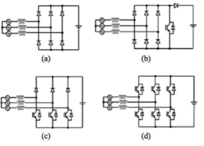
(20) CHAPTER 2. BACKGROUND. 7. The main components of a wind energy conversion system are the blades, the generator, power conversion devices (AC/DC), a dc bus capacitor, and an inverter (DC/AC conversion) for grid connection. [10]. 2.1. Generator. A wind turbine can be equipped with any type of three-phase generator. Generators convert the kinetic energy from the wind to mechanical work. Different sets of configurations can be made such as squirrel cage rotor induction generator, dual-stator induction machine (DSIM), doubly fed induction generator (DFIG), brushless doubly-fed machine with several structures (BDFM), synchronous generator with external field excitation and permanent magnet synchronous generator (PMSG), among others. [6] Each generator has benefits and drawbacks and must be connected with different devices, but the field of small generation is dominated by the use of asynchronous generators directly connected to the grid/load and more recently by PMSGs with diode rectifiers, boost converter and inverter [8]. The PMSG configuration has two topologies. The first one consists of an uncontrolled rectifier, and a DC/DC converter and the other type is a controlled rectifier. The one that uses a controlled rectifier and inverter is known as back-to-back converter. [11]. 2.2. AC/DC Converters. These devices convert the AC output of the generator to DC and are controlled by the MPPT system to maximize the generator output power as the wind speed changes. An energy storage unit can also be added to the output of the AC-DC converter to store excess energy or a DC-AC converter if the system is grid-connected. AC-DC converters work with a controller depending on the topology, and they should be available to achieve the next objectives: 1. Convert the AC output of the generator to DC. 2. Control the generator to produce a desired torque or power at high efficiency. 3. Offer high performance, low cost, high efficiency and simple control. There are four main types of AC-DC converters: rectifier, single-switch switched-mode rectifier (SMR), semi-bridge SMR and inverter [10]. Their configurations can be seen in Figure 2.2..

(21) CHAPTER 2. BACKGROUND. 8. Figure 2.2: Main types of AC-DC converters for PM generators. (a) rectifier. (b) single-switch SMR, c) semi-bridge SMR and (d) controlled rectifier. Retrieved from [10] The rectifier(Fig.2.2a) is the simplest and the lowest cost converter among the four converter types. It uses six diodes and cannot be controlled. It can neither produce power at low winds speeds nor achieve maximum power tracking. The second converter (Fig.2.2b) is a simple single-switch SMR that consists of a threephase uncontrolled rectifier and a boost switch. Figure2.2c shows the semi-bridge SMR topology. This configuration uses three lower switches in the power circuit, which can be separately controlled. Its downside is that it has a weak performance at low speeds. The last configuration is the well-known controlled rectifier topology, which contains six switches. This converter offers the highest output power capacity at low speeds since it is fully controlled and it offers a significant advantage in speed control.. 2.3. DC/AC Converters (Inverters). Since the voltage and frequency of the AC generated by the wind turbine are variable and depend on the wind speed, it cannot be delivered to the grid without the correct phase or voltage. To be exported to the utility grid the power needs to be converted to the frequency and voltage level of the grid. These devices are used to achieve this conversion, also known as DC to AC inversion. This conversion is done in 2 steps: • The 3-phase AC voltage from the generator is filtered and converted to the DC voltage. The topologies mentioned previously are used for this type of conversion (rectifier, controlled rectifier, etc.)..

(22) CHAPTER 2. BACKGROUND. 9. • The resulting DC output is connected to the grid via inverters that supply the correct voltage and phase.. 2.4. Control Strategies. In regards of control engineering research has several trends. There are different types of controllers that try to achieve different goals, such as, maximum power control tracking (MPPT), load control, mechanical damage reduction, wind estimation, among others. The types of control go from a standard PID scheme to fuzzy logic and adaptive strategies, to name a few. In 2011 an overview was presented listing these types and the possible future directions [4]. Table 2.1 Control Strategies used in Wind Power Systems. Control Strategies Overview Control Method PID Control Optimal Control Hard Control Adaptive Control Sliding Mode Control Predictive Control Fuzzy Control Soft Control Neural Networks Control Fuzzy and PID Control Fuzzy and PID Control Neural Networks and PID Hybrid Control Fuzzy and Genetic Algorithms Fuzzy and Adaptive Control Fuzzy and Sliding Mode Control Adaptive, Fuzzy and Sliding Mode Control Fuzzy and Neural Networks and Sliding Mode Control Control Type. Each controller has positive values and disadvantages, and they are chosen according to the situation at hand. The system configuration, the process variable, and the objective of the controller are critical when designing a control topology. For example, variable speed and fixed pitched wind generation systems usually use speed and torque control [11]. Both of them are achieved through current variations as stated in chapter 1. Several issues are stated in [4], and it can be concluded that every controller will have a downside, but the selection must be made in order to reach the objective in hand and to follow the best possible operation..

(23) CHAPTER 2. BACKGROUND. 2.5. 10. Operation. Variable speed wind turbine operation is divided into three regions. Region 1 is start-up and it lasts very short time. In this region, the wind speed is too low, and the power available in the wind is low compared to losses in the turbine system. Hence, the turbines are not run. This region will not be analyzed in this research.. Figure 2.3: Variable Wind Turbine Regions. Retrieved from [9] Region 2 is the gap where the wind is not strong enough to bring the generator to rated speed, so the maximum power capture that the wind can offer is desired. Aerodynamic losses prevent the turbine from achieving its maximum theoretical power extraction from the wind, called the Betz Limit, but the goal is to approach that curve as closely as possible. The strategies and experiments implemented in this research focus on this region. Region 3, on the other hand, is where the wind is very strong and the generator is already at its rated speed, so actions must be taken to limit the power output to avoid exceeding safe electrical and mechanical load limits.. 2.6. Maximum Power Point Tracking (MPPT). Each wind turbine design has a unique associated power coefficient function Cp that describes its power extraction efficiency. The kinetic power in the wind is converted to mechanical power that is extracted by the wind turbine and its behavior is dictated by the next equation. P = 0.5ρACpV 3. (2.1). Where V is wind speed [m/s], ρ is air density [kg/m3 ] and A is rotor swept area [m2 ] meaning.

(24) CHAPTER 2. BACKGROUND. 11. that the mechanical power developed depends on these factors. The power coefficient is dependent on two parameters: the tip speed ratio (TSR) given by λ, and the pitch angle given by β . For wind turbines with a fixed pitch, the value of is zero. The maximum value for the Cp will correspond to a different TSR for each pitch angle [19]. Therefore, to obtain the maximum power point, one must use the maximum value of the power coefficient for each tip speed ratio.. Figure 2.4: Cp vs. λ Curve The mechanical power can be plotted as a function of the rotor speed for different values of the wind speed. The rotor speed in which the maximum value for each wind speed is achieved is known as the MPPT curve.. Figure 2.5: Example of Power vs. rotor speed Curve. Retrieved from [8]..

(25) CHAPTER 2. BACKGROUND. 2.7. 12. Testing and Monitoring Facilities. Several papers on monitoring facilities regarding wind turbine systems show advancements on reading the AC and DC signals using a DAQ device and LabVIEW software in order to display the signals in real time. These installations are usually used on small wind turbine systems and for testing purposes in a controlled environment. [14-18]. Field installations have a more complex instrumentation system, and recent investigations show that there is a recent increase in wireless technology used in these types of systems in order to achieve a remote reading of the signals. Wireless installations are usually cleaner, cheaper and easier to maintain. [14-18] LabVIEW applications dominate the test system field and these types of facilities inspired the design of the monitoring system that was used in this research. Monitoring facilities can offer measurements that can help understand the systems dynamics compute its efficiency and register the measured values.. 2.8. System Identification. The identification of wind energy conversion systems (WECS) has been widely discussed in the literature, and it often depends on different identification algorithms and techniques. It goes from generator parameter identification, AC/DC converter identification, or a back-toback identification [13,20-22]. The identification process can be made offline or online, and the techniques change accordingly. For example, an offline process can be made with a Pseudo Random Binary Sequence (PRBS) by analyzing the given dataset with the appropriate algorithms or software [20]. On the other hand, an online identification can be achieved by reading each new value of the systems inputs and outputs with recursive algorithms such as the recursive least squares (RLS) [13]. The emphasis of more recent research has been more toward the development of online model identification techniques [13]. The least squares (LS) algorithm and the PRBS are often used together because the PRBS gives a set of values that provide significant information about the system, and the LS provides a reliable model that follows the systems dynamics. For example, David K et al. [22], used both to identify a power conversion system. The identified models are often used for controller design or simulation purposes.. 2.9. Predictive Control. Predictive control refers to a class of computer control algorithms that utilize an explicit process model to predict the future response of a plant. The algorithm attempts to optimize future.

(26) CHAPTER 2. BACKGROUND. 13. plant behavior by computing a sequence of future manipulated variable adjustments. [32] Predictive control provides a good setpoint tracking behavior and disturbance regulation techniques even when constrained. In cases where dead time and reference trajectories are known, predictive control establishes a faster performance compared with PIDs. As defined by Jose Rodellar in [34], predictive controls general idea can be summarized in the next sentence. Based on a model of the process, predictive control is the one that makes the predicted process dynamic output equal to a desired dynamic output conveniently predefined.. Figure 2.6: Basic Predictive Control Diagram. Retrieved from [34]. 2.10. Adaptive Predictive Control. Wind systems are typically nonlinear and time-varying because of the characteristics of the wind and the components that compose them. They are subjected to disturbances, vibrations, and sudden changes that when addressed by a constant model, it fails to mitigate the unwanted effects. All the systems that present time-varying dynamics inspired this type of controllers. This control extends the conventional predictive strategy and adds an adaptive mechanism that uses new information to change the predictive model to optimize the predicted and real outputs. Since wind systems are complex and hard to model, this technique amends any modeling errors and unknown perturbations.. Figure 2.7: Basic Adaptive Mechanism. Retrieved from [34].

(27) Chapter 3 System Overview This research focuses on the optimization of a PMSG small wind turbine with variable speed. It uses a six-pulse control rectifier, a dc bus capacitor, and a commercial inverter to provide the back-to-back conversion. Classic, predictive and adaptive-predictive control strategies were chosen with an MPPT focus for region 2 and experiments were conducted on a laboratory installation using the components mentioned previously. Prior to designing the controller or the power electronics, preliminary work had to be made in order to achieve a correct experimentation. A system where the user had the ability to manipulate the angular speed of the generator, monitor power, and voltage outputs, and connect the system to the grid was needed. The required instruments, applications, and devices to accomplish the preceding objective were assembled, thus giving birth to the test facility. Table 3.1 System Components Component Model Data Acquisition Device NI DAQ 6212 Variable Frequency Drive Yaskawa Varispeed A100 Three Phase Motor Sumitomo Sm-Cyclo 1K-FX PMSG Richuan Wind Power - 2kW - 300 Rpm ACD/DC Converter Custom Made AC Voltage Transducer VT7-010X5 DC Voltage Transducer VTU-010X5 AC Current Transducer CTL/CTA 201HX5 Signal Frequency Transducer VT7-016X5 Microcontroller Arduino Due Dc Bus Capacitor Cornell Dubillier, Film Capacitor, 947D-880µF DC/AC Inverter 3.6 - PVI-OUTW AURORA Load 5-100 Ω Torquemeter LoadStar Sensor 200 lbf Capacitive Loadcell Ω. 14.

(28) CHAPTER 3. SYSTEM OVERVIEW. 15. A computer runs a LabVIEW application that is used to manage inputs and outputs through a data acquisition device NI DAQ-6212. The device sends an analog output to a variable frequency drive (VFD) that controls the rpm of a three-phase motor. This motor is coupled to the PMSG, and its rotation emulates the blades movement. The PMSG spins and produces three-phased electrical energy that connects to the controlled rectifier and to the transducers directly. There are a voltage transducer and a current transducer for each of the phases of the PMSG, one that senses the frequency of the generated signal, and others that sense DC voltage and current. Each of these transducers serves as an input for the NI DAQ-6212 and the application shows in real-time measurement values of each variable. The six-pulse rectifier is controlled by power electronics and a microcontroller that sends the information of the rectifiers firing angle, as it will be explained in the following chapters. The microcontroller senses the DC voltage, DC current, signal frequency and the intersection between phases and it uses this information to compute the angle.. Figure 3.1: System Overview The DC output of the controlled rectifier goes to a DC bus capacitor that reduces the ripple in the signal. The capacitor is wired directly to the Aurora inverter. The inverter then redistributes the energy to the grid. The physical installation is divided into three major sections: mechanical assembly, circuitry and rectifier cabinets, and the transducer panel..

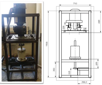
(29) CHAPTER 3. SYSTEM OVERVIEW. 3.1. 16. Mechanical Assembly. This section is the mechanical installation and the coupling of the three-phase AC motor with the gearbox and finally, the PMSG. The set consists of a vertical arrangement that holds the AC motor in the upper part, a gearbox in the middle and the PMSG in the bottom. The upper body of the installation has a moving mechanism that is used to position the AC motor on the same axis as the PMSG.. Figure 3.2: Mechanical Assembly The mechanism consists of two handles made by two endless screws that push and pull the table in which the motor rests. The screws provide millimetric movement at a high precision rate that enables a high-quality alignment. A correct alignment is required to reduce any losses.. Figure 3.3: Moving Mechanism.

(30) CHAPTER 3. SYSTEM OVERVIEW. 17. Additionally, the generators base has a concentric shaft on its bottom side that works like a rotor extension in which a momentum arm is installed. This arm rotates along with the generator, and its end pushes a load cell sensor that registers the force produced by the PMSG. The arms length and the registered force are used to calculate the generators electromagnetic torque.. Figure 3.4: Torque Sensor. 3.2. Circuitry and Rectifier Cabinet. The circuitry cabinet contains the circuits power supply, a voltage divider circuit, the microcontroller and the trigger control circuit. The power supply is used to power the trigger circuit and the voltage divider. Furthermore, the microcontroller computes the firing angle delay, and the circuit generates the pulses for each of the thyristors on the controlled rectifier.. Figure 3.5: Control Circuitry (Left) and Control Rectifier (Right).

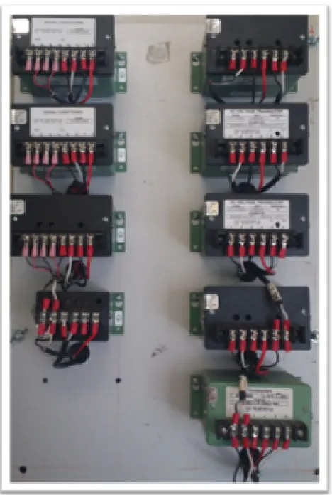
(31) CHAPTER 3. SYSTEM OVERVIEW. 18. At the same time, the rectifier uses the pulses and the three-phased signals to rectify the signals and obtain VCD and ICD. Moreover, the thyristors are installed over a heat sink to prevent any high-temperature malfunctions, and all the voltage inputs have a fuse security measure to prevent any overcurrent problems.. 3.3. Transducer Panel. As previously mentioned, the transducers are used to measure the voltages, currents, and frequency of the generated signals. A transducer panel was installed to wire each of the input signals and then supply them to the data acquisition device to monitor them on the LabVIEW application. This modules objective is to provide the needed signals in real-time to the data acquisition device to enable a computer-based monitoring facility. It provides the measurements that are going to be registered in the systems database. Nine transducers assemble the panel. Three for AC voltage, three for AC current, one for signal frequency, one for DC voltage and one for DC current. The distribution of the transducer panel can be seen in figure 16, and their description can be seen in table 3.2. Table 3.2 Transducer Model and Output Range Measurement Sensor Output Phase A Voltage DC VOLTAGE TRANSDUCER VT7-010X5 (VA) ±5v Phase B Voltage DC VOLTAGE TRANSDUCER VT7-010X5 (VB) ±5v Phase C Voltage DC VOLTAGE TRANSDUCER VT7-010X5 (VC) ±5v Phase A Current CTL/CTA 201HX5 SIGNAL CONDITIONER (IA) ±5v Phase B Current CTL/CTA 201HX5 SIGNAL CONDITIONER (IB) ±5v Phase C Current CTL/CTA 201HX5 SIGNAL CONDITIONER (IC) ±5v Rectified Voltage DC VOLTAGE ISOLATOR VTU-010X5 (VDC) 0-5v Shunt Current DC VOLTAGE TRANSDUCER VT7-016X5 (IDC - SHUNT) ±5v Signal Frequency TRANSDUCER AFT-065X5 0-5v Torque LOADSTAR SENSOR (250 lbf) NA. 3.4. Electrical Installation. All the system devices such as inverter, VDF, computer, transducer and generator must be grounded to prevent any current leakage and ground faults..

(32) CHAPTER 3. SYSTEM OVERVIEW. Figure 3.6: Transducer Panel. 19.

(33) Chapter 4 Maximum Power Point Curve Design The primary control objectives for a wind energy system is to maximize the energy capture. As previously mentioned, the mechanical power captured by the wind by any turbine is given by equation (1). The retrieved power is linked to the aerodynamical characteristics of the wind turbine, and since the air density and the area can be assumed constant, the output power is only influenced by the Cp curve. The WECS used for this research consists of a horizontal axis, variable speed, fixedpitched system (β=0), therefore the power constant depends only on the tip speed ratio given by the following equation: [25] Rω (4.1) V Where V is wind speed [m/s], R is rotor radio [m] and is angular speed [rad/s]. The intention is to keep the turbine operating at the peak of its Cp-TSR-Pitch surface, so Cpmax is desired. Since generators rotational speed goes from 0-300 rpm and the wind speeds go from 5-10 m/s, a set of values for λ can be calculated for each rotational and wind speed. λ=. Figure 4.1: Typical Cp vs. λ Curve.. 20.

(34) CHAPTER 4. MAXIMUM POWER POINT CURVE DESIGN. 21. The Cp curve is typically given in the form of figure 4.1 and its values can be found by using the TSR and information from the manufacturer. The optimum value for Cp and can be found on the maximum values of Cp and this group of values is used to compute the maximum power retrieved from the wind. Although the value of the Cp curve is a parameter that is usually given, it is different for every turbine and a convenient way to reproduce the curve is given in [30,31] using equations 4.2 and 4.3. C p = a1 (. −a5 a2 − a3 β − a4 )e λi λi. (4.2). 1 1 b2 = − 3 (4.3) λi λ + b1 β β + 1 The coefficients a and b were chosen to fit a 1.2 kW wind turbine with the operation parameters mentioned before. Since there is no pitch angle (β=0) equation 4.3 yields λi = λ and the used coefficients are a1 =3.86,a2 =5.5,a4 =022 and a5 =7. A density value of 1.2998 kg/m3 , a rotor radius of 1 m and equations (2.1-4.3), were used to obtain the mechanical power offer for each wind speed. As previously mentioned, each wind speed will have an optimal Cp that when replaced on equation 2.1 the maximum power point is obtained, therefore generating the maximum power curve.. Figure 4.2: Typical Cp vs. λ for every Vwind and ω The values for each of the maximum points can be seen in table 4.1, and the behavior of the winds mechanical power for each rotation speed can be seen in figure 11. Table 3 offers information about the relationship between the optimal rpm values, the optimal Cp values and the maximum power points for each wind speed. The obtained rpms will be used as the set.

(35) CHAPTER 4. MAXIMUM POWER POINT CURVE DESIGN. 22. point of the controller in order to achieve the MPPT. Table 4.1 Maximum Power Points Wind 5 MPPT 84.2 Cpopt 0.33 RPM 147. 5.5 6 112 145 0.33 0.33 161.8 176.4. 6.5 7 185 231 0.33 0.33 191.2 206. 7.5 8 8.5 284 345 413 0.33 0.33 0.33 220.2 234.8 250.2. 9 9.5 10 491 577 674 0.33 0.33 0.33 264.4 279.4 294. Figure 4.3: Mechanical Power Offer with Maximum Power Points. 4.1. Speed Control. The previous analysis shows that there exists a relationship between the rotational speed and the extracted power output. In order to find the desired power output, an rpm control strategy must be designed. In a variable wind speed conversion system, the rotor is driven by the torque given by the aerodynamical conditions of the turbine τa , and braked by the generators electromagnetic torque τem . The mechanical speed dynamic equation is given by: [27,28]. dΩ ) = τa − τem (4.4) dt Where JT is the equivalent moment of inertia, τa is the aerodynamical torque, τem is the electromechanical torque and ( dΩ ) is the rotors acceleration. From equation 4.4, it can dt JT (.

(36) CHAPTER 4. MAXIMUM POWER POINT CURVE DESIGN. 23. be concluded that the rotors acceleration and consequently its rotational speed can be set in a desired point by controlling the electromagnetic torque of the generator. Moreover, the electromagnetic torque is directly proportional to the generated current and voltage, therefore if a generated voltage and current control is used, a rotational speed control can be achieved. The next chapter explains how the voltage and current control is generated. In order to achieve the steady-state operation of the generator, the aerodynamic and electromechanical torque must be balanced so that acceleration equals zero. It is then that the rotational speed will be constant and therefore a constant power value is achieved. The implementation and explanation of the algorithm that controls the rotational speed will be seen in chapter IX. As mentioned in the system overview, a commercial inverter connects the generated power with the grid. This commercial device has a voltage input-power output relationship that enables the grid connection. In order to work efficiently, one must obtain the voltage power curve that will be inscribed in the inverter. Since table 4.1 relates the rotational speed with the maximum power value, calculations must be made to find the DC voltage value that goes along with the optimal rotational speed for a given wind speed.. 4.2. Voltage-Power Curve Design. In order to find the needed voltage from the rotational speed and power, one must use several equations and relate several concepts. Preliminary work was needed to find the generators parameters and its power offer and demand dynamics. Open loop tests were run for a set of rotational speed values and different DC loads that dissipated the generated powered and simulated the power demand. The values for phase voltages, line-to-line voltages, DC current, DC voltage, rotation frequency, the used loads, the rectifier efficiency, the three-phased efficiency and the overall efficiency, among others, were registered and a vast collection of data was generated. All off these values depend directly on the rev/min and the value of the applied load; therefore, a correlation between all of them can be made. The way that the power offer is dissipated in the loads is known as the power demand, and it is the first step in the way to find the values of the required voltage. The power demand can be plotted along with the offer and the maximum power points, and the figure suggests that the maximum power values can be placed within the maximum and minimum demand constraints of the whole system..

(37) CHAPTER 4. MAXIMUM POWER POINT CURVE DESIGN. 24. Figure 4.4: Mechanical Power Offer (Black) and Demand (Colored). The variety of the tests goes from a 50-300 rpm range with 50-rpm steps and a value of loads from 5 ohms to 100 ohms. An interpolation can be made inside this range of values in order to cover the whole spectrum with a better resolution and find the value of rotational speed and load that gives each desired power output.. Figure 4.5: Mechanical Interpolation The rest of the measured values are also interpolated and the registered values are used to find the respective DC Power. The DC power is obtained by multiplying the mechanical power by the efficiency of the whole system. This efficiency values can provide the behavior of the conversion system. ηtotal =. Pdc (rpm, Rl) Pmec (rpm, Rl). (4.5).

(38) CHAPTER 4. MAXIMUM POWER POINT CURVE DESIGN. ηtotal ∗ Pmec (rpm, Rl) = Pdc (rpm, Rl). 25. (4.6). Once the DC power is obtained, Ohms law provides the last relationship given by the following equation. Pdc (rpm, Rl) = Vdc (rpm, Rl) =. p 2. Vdc2 Rl. Pdc ∗ Rl. (4.7) (4.8). The found values are the voltage inputs for the commercial inverter that connects the grid with the wind energy conversion system. By using these parameters, two equations can be obtained. One plots the mechanical power for each rpm value, therefore yielding the MPPT and the other one provides a relationship between the wind speed and the desired voltage input for the inverter. P mec = 0.0004065Rpm3 − 0.01314Rpm2 + 0.7544Rpmm − 0.3473 2 Vdc = −0.02805VW3 ind + 0.03428Vwind + 13.58051VW ind − 0.0010756. (4.9) (4.10).

(39) Chapter 5 AC/DC CONVERSION This chapter explains how does a controlled rectifier work, the equations that dictate its behavior and how is it used in the WECS. The design and component selection of the device are beyond the objectives of this research, and therefore it will not be explained.. 5.1. Controlled Rectifiers. Controlled rectifiers are line-commutated ac to dc power converters, which are used to convert a fixed voltage, fixed frequency ac power supply into a variable dc output voltage. By employing phase controlled thyristors in the controlled rectifier circuits, one can obtain variable dc output voltage and variable dc output current by varying the trigger angle at which the thyristors are triggered. In contrast to a diode, a thyristor does not automatically turn ON at the instant in the AC cycle at which it becomes forward biased. Control of the DC output is achieved by adjusting the delay time, usually expressed in angular measure, of the gate firing pulse to each thyristor from the instant it would have turned ON had it been a diode. The thyristors are forward biased during the positive half cycle of the input supply and can be turned on by applying suitable gate trigger pulses at the thyristor gate leads. The current begins to flow once the thyristors are triggered at the angle . The output voltage across the load follows the input supply voltage through the thyristors. When the load current falls to zero, the thyristor turns off due to AC line or natural commutation. They remain off during the negative half cycle of the input supply. These devices can be classified into two different types 1. Single Phase Controlled Rectifiers, which operate from single-phase ac input power supply. • Half-wave controlled rectifier. – Uses a single thyristor device, therefore providing output control only in onehalf cycle of the input ac supply. • Full-wave controlled rectifier. 26.

(40) CHAPTER 5. AC/DC CONVERSION. 27. – Single phase semi-converter: ∗ Half controlled bridge converter, using two SCR’s and two diodes. – Single phase full-converter: ∗ Fully Controlled bridge converter, which requires four SCRs. 2. Three Phase Controlled Rectifiers, which operate from three-phase ac input power supply. • Three-phase half wave controlled rectifiers. • Three-phase full wave controlled rectifier. – Semi converter (half controlled bridge converter). – Full Converter (fully controlled bridge converter). The chosen configuration for this research consists on a three-phase full wave controlled rectifier with a variable frequency input.. Figure 5.1: Fully Controlled Three Phase Rectifier. 5.2. Controlled Rectifiers. A three-phased controller is a fully controlled bridge controlled rectifier using six thyristors connected in the form of a full A wave bridge configuration. All the six thyristors are controlled switches, which are turned on at appropriate times by applying suitable signals. The thyristors are triggered at an interval of 60◦ and they are numbered in figure 5.1 in the respective order in which they are triggered. The firing sequence of the thyristors is 12,23,34,45,56,61,12,13 and so on..

(41) CHAPTER 5. AC/DC CONVERSION. 28. Figure 5.2: Firing Sequence The input parameters are three line-neutral voltages and three line-to-line voltages defined by the following g equations and the rectifiers behavior can be seen in 5.3. Vcn. 5.3. Van = Vm sin(ωt) 2π Vbn = Vm sin(ωt + ) = Vm sin(ωt − 120◦ ) 3 2π = Vm sin(ωt + ) = Vm sin(ωt + 120◦ ) = Vm sin(ωt − 240◦ ) 3 √ π Vab = (Van − Vbn ) = 3Vm sin(ωt + ) 6 √ π Vbc = (Vbn − Vcn ) = 3Vm sin(ωt − ) 2 √ π Vca = (Vcn − Van ) = 3Vm sin(ωt + ) 2. (5.1) (5.2) (5.3) (5.4) (5.5) (5.6). DC/AC Voltage Relationship. In the general case of a n-pulse rectifier, the DC component of the output voltage can be determined by taking the average over one repetitive period of the waveform of the output terminal voltage. In this case, the output load voltage consists of 6 voltage pulses over a period of 2 radians, hence the average output voltage is calculated as: Z π +α 2 6 Vdc == Vab dωt 2π π6 +α √ π Vab = 3Vm sin(ωt + ) 6 ∴. (5.7) (5.8).

(42) CHAPTER 5. AC/DC CONVERSION 3 Vdc = π. Z. 29. π +α 2. √. π +α 6. 3Vm sin(ωt +. π )dωt 6. √ 3 3Vm Vdc = cos(α) π. (5.9) (5.10) √. m For a diode rectifier the delay angle is zero, therefore, its output value is equal to 3 3V . On the π other hand, the root mean squared (RMS) values were found using the following equations. s Z π +α 2 6 VRM S = V 2 dωt (5.11) 2π π6 +α ab. s Z π 3 2 +α 2 2 π VRM S = 3Vm sin (ωt + dωt π π6 +α 6 √ √ 1 1 3 3 cos(2α)) 2 VRM S = 3Vm ( + 2 4π. Figure 5.3: Three Phase Controller Rectifier Inputs and Outputs, α =. (5.12). (5.13). π 3.

(43) CHAPTER 5. AC/DC CONVERSION. 5.4. 30. Control Rectifier Testing. The device was tested meticulously to verify its performance for a broad set of firing angles with several signal frequencies. Its behavior was compared with the theoretical values of the dc output given by equation 5.10. As seen on figure 5.4 it is possible to control the rectified voltage by changing the firing angle for every available frequency or rotational speed. This way, the rectifier adopts the role of the actuator of the closed-loop system because it executes the control actions to change the processs output. The voltage control achieved by the rectifier can be used to control the systems power outputs as well. As mentioned in chapter IV, rotational speed and the firing angle are inversely proportional. As the firing angle increases, the electromagnetic torque decreases. The torque is directly proportional to the DC current and when the rectified current and voltage change, the torque changes accordingly. Therefore, following the dynamics of equation 4.4, if the rotation speed needs to be increased the firing angle is lowered; on the other hand, if it needs to be decreased the firing angle increases.. Figure 5.4: VCD and ICD vs Alpha The results obtained from the tested device conclude that there can be a control strategy focusing on power and rotational speed can be achieved by manipulating the systems secondary variables. Now that the AC/DC side is covered, the DC/AC strategy must be analyzed..

(44) Chapter 6 DC/AC Conversion This chapter explains the inverter configuration, its capabilities, its composition and the way it is designed. The electrical configurations, power curve inscription, power input and output monitoring and software installation is also covered.. 6.1. Aurora Inverter Description. The Aurora inverter has as its primary function to connect the generated voltage to the electric grid with the correct frequency and voltage level. It also allows the user to ensure a power output control with a predesigned behavior. The devices main elements are the input DC-DC booster converters that raise the voltage level when needed and the output inverter that produces the AC voltage output. It also has a varistor bank on its VDC input to reduce the ripple in the rectified voltage, consequently making its power control more efficient. The selected model is a PowerOne PVI-3.6-OUTD-US-W, and with a transformerless configuration to reduce conversion losses. This model has an input range of 0-580 Vdc and 0-10 Adc. It requires at least, 50 volts on its input to establish the grid connection initially.. Figure 6.1: Aurora Inverter Electrical Diagram. 31.

(45) CHAPTER 6. DC/AC CONVERSION. 32. The aurora has 2 DC inputs on its lower left side that are connected in parallel and a three-pinned AC output on its right side that must be wired in accordance with the electrical configuration of the country in which it will be used. A three-phase star connection was used in this configuration.. Figure 6.2: Aurora’s AC output configuration The inverter uses a P-V curve to ensure the power output. Nevertheless, this curve must be written in the auroras processor by establishing a communication between the device and the controller unit. The Aurora supports an RS232/485, Ethernet or USB communication protocols, each of with different capabilities.. Figure 6.3: Communication Protocols. 6.2. Data Communication and System Configuration. The selected configuration used the RS485 protocol through a RS485/RS232 adapter and a USB-RS232 adapter. The PowerOne software and drivers are required to enable the devices correct performance. The required software and and their use are presented in table 6.1..

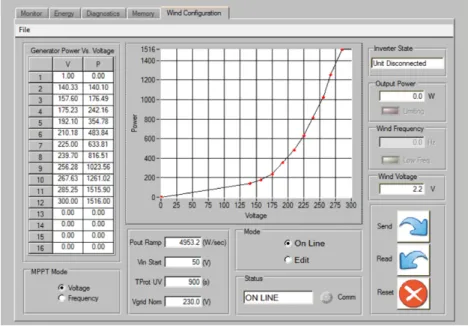
(46) CHAPTER 6. DC/AC CONVERSION. 33. Table 6.1 Required Drivers and Software Component FTDI USB-RS485 ADAPTER TUSB3410 Driver FTDI VCP Driver FTDI D2XX DRIVER Aurora Installer Aurora Communicator. Description USB-RS485-WE-5000-BT Enables the USB To Serial Communication Virtual COM port (VCP) drivers cause the USB device to appear as an additional COM port available to the PC. Allows direct access to the USB Device through a DLL. Aurora-Computer Communication Aurora-Computer Communication. Additionally, the PowerOne software was used to monitor and to configure the operation of the inverter. The Aurora Installer allows the user to view, select and display the COM port where the device is connected and the communication protocol to be used. If the said port is selected, the software provides an interface in which the systems status can be monitored, access the memorys data log is enabled, the option to see input and output information is presented and finally a way to inscribe the P-V curve is available. The P-V curve screen can only be accessed in the extended mode of the aurora installer. This screen provides the ability to read the current power table, write a new power table or reset the configuration. It can also change the rate with which Pout changes, the grid voltage and the MPPT mode. The used configuration can be seen in figure 27.. Figure 6.4: Wind Configuration Window (Aurora Installer).

(47) CHAPTER 6. DC/AC CONVERSION. 6.3. 34. Data Communication and System Configuration. It is important to mention that the curve used in the Aurora works like the systems centerpiece. Moving the firing angle will also change the mechanical power demand and all the values obtained from this curve (mechanical power, torque, VCD, ICD, among others). Therefore, a different P-V curve for each firing angle can be obtained. If a P-V curve is already inscribed in the device, moving the firing angle will change how the power is delivered. The available range is the same as the firing angles (0-90) and an increase in the angle will move the curve to the right while a decrease will move it to the left. A middle ground should be selected in order to provide equal displacement to the left and the right so that the curve can be indirectly modified. Figure 6.5 shows this phenomenon.. Figure 6.5: Mechanical Power, Alpha Change. 6.4. RS485 Wiring. The Aurora has an internal memory to save information such as events, alerts, errors or for datalogging purposes. Another way to save the systems data (input and output power), the software provides a datalogging option. A permissible sampling time, a memory location, the measured variables and the type of file have to be defined in order to enable the option. Moreover, the data logging option is only available if a communication channel with the computer is enabled. The selected communication protocol was the RS485-USB communication, because it provides an easy installation, a plug and play experience and a fast data transfer. To enable the RS485 communication, the terminal T/R+ should be connected to the Orange terminal of the USB-RS485 adapter, the T/R- to the Yellow terminal and finally RTN.

(48) CHAPTER 6. DC/AC CONVERSION. 35. to the black terminal on the Inverter.. Figure 6.6: USB485 Connections. 6.5. Test Results. The DC-DC converters of the device carry out the current management on the grid side. If the generated power is not enough the Aurora will take a control action on the current in order to achieve the power in the inscribed curved. The device was submitted to several voltage changes to verify that the needed power was delivered correctly, and the results were saved using the data logger option inside the device. The test consisted on several voltage setpoints and measuring the output power displayed by the device.. Figure 6.7: Voltage input and Power output.

(49) Chapter 7 System Identification System identification is the process of characterizing the behavior of a real process in order to reveal and better understand its cause-effect relationships. A mathematical model that emulates the essential aspects of the behavior gives this relationship, unfortunately it is not always easily found. In control theory, it is necessary to know the process that is going to be manipulated in order to design an efficient controller. The model is typically found by analyzing the experimental input-output data of the process. Several methods can be used to obtain the stated relationship, such as Ziegler-Nichols, step-response and impulse response, to name a few [12].. Figure 7.1: Identification Process Identification techniques can be used to find a continuous-model in the Laplace-domain or for a discrete-model in the Z-domain. When the control strategies are going to be handled by a digital device, the identification must be made in the Z-domain and written as a difference equation.. 36.

(50) CHAPTER 7. SYSTEM IDENTIFICATION. 37. The stated techniques offer a very limited set of information about the process and although sometimes it is enough to control simple processes, more complex systems require a more sophisticated method. For example, step response methods present the following disadvantages: • Low precision. • Ignores the effect of disturbances. • Outputs a continuous-time model that requires discretization. • Discretization errors appear. Since the control strategies are going to be executed from a microcontroller, a discrete-time model must be obtained, and discrete time identification must be made. A pseudo-random binary sequence (PRBS) can provide this type of identification.. 7.1. PRBS. The PRBS consist of a random sequence of binary states and is usually generated using a shift register with feedback paths. The length of the sequence (N) is dependent on the number of bits (M) of the shift register and the positions of the feedback paths [13]. Figure 7.2 shows a PRBS with a 5-bit register of length L = 2N − 1 = 25 − 1 = 31.. Figure 7.2: 5-bit PRBS Representation This type of identification gives a more complete response of the system because the input of the system has the properties of white noise, in other words, a high content of frequencies. The information delivered by the test gives a good understanding of the behavior of the system at several frequencies. They achieve this by changing the duration of a pulse every run. It is important to mention that the maximum duration of a pulse is equal to N. The processs gain can be identified correctly if the duration of at least one of the pulses is greater than the rising time of the process. Meaning the condition tr < N ∗ T s, where Ts is the sampling time, must be followed. This condition helps determine the value of N and therefor the length of the PRBS..

(51) CHAPTER 7. SYSTEM IDENTIFICATION. 38. Figure 7.3: PRBS Pulse Length. 7.2. PRBS Design. When designing a PRBS the number of registers and the sampling time must be defined. A way to do it is to run a step response test to see the rising time of the system and proceed to select the N and the sampling time accordingly. Since the systems dynamics change with every wind speed, several step responses were made to organize the dynamics in regions that fit the winds velocity range. Since the experimentation system emulates the wind with a motor, different sets of rpms were selected to emulate different wind speeds. The results of chapter 2 show that the area of interest starts at 150 rpm since the first maximum power point is found around that rotational speed. Consequently, the selected speeds go from 150-300 rpm. The value changes were taken on the controlled variable, which is the firing angle of the rectifier, in addition, the voltage and currents produced were registered. The change in the input variable was from the 0% to the 100% which means a firing angle of 60◦ to 5◦ , therefore creating a maximum firing angle of 60◦ . The experimental data was analyzed using the control station software to obtain the time constant of each configuration. Control theory defines rising time as the time taken by a signal to change from a specified low value to a specified high value. A first-order system gets to the 63% value after a time constant τ has passed and it reaches steady state after 4 τ have passed. Since the steady state value is the specified high value of the system, it can be concluded that 4 τ is also the systems rising time..