Statistical Cellular Scatter Density Model (GSDM ) Employing Smart Antennas dor Macrocell Environments Edición Única

Texto completo

(1)Chapter 1 Introduction The tremendous growth in technology has led many applications in wireless communications. To provide high quality services and to increase capacity in wireless systems, improved methods to combat multipath effects must be developed. Then a study of the spatial properties of the received fading signal becomes necessary, in order to have spatial channel models that describe the parameters of the multipath components [1]. There. are. three. important. parameters. that. characterize. a. channel. of. communications: •. The power of the multipath components.. •. The AOA of the multipath components.. •. The TOA of the multipath components.. This thesis deals principally only with one of this parameters the AOA, because a deeper study would be necessary if we want to include more characteristics, but a simulation taking into account the power of the multipath components is also made. The use of antennas arrays at the BS permits the improvement of system performance. Recently, there has been intensive research on smart antennas in mobile communications for exploiting the spatial domain, example, null steering for isolating cochannel users; optimum combining for reducing multipath fading and suppressing interference; and beam steering for focusing energy toward desired users.. 1.

(2) Chapter 1. Introduction. Thus smart antennas are a promising technology for increasing capacity in macrocellular and microcellular systems.. 1.1 Objective The goal of this investigation is to characterize the behavior of the PDS in a Gaussian scatter environment when arrays of antennas are deployed and compare the results with the previous studies in omnidirectional and sectorized antenna. Obtain a relationship between the AOA at the BS and the Doppler frequencies with the thought of add different gains that affect the shape of the spectrum. Simulate the GSDM and include a model of propagation due the distances among the MS to the scatter and from the scatter to the BS and observe the effect on the PDS.. 1.2 Justification Due to the importance of satisfying the demand of knowledge in an emerging area like smart antennas any contribution is worthwhile. This thesis has been made to observe the improving on the PDS when arrays of antennas are using. The PDS is using to calculate the LCR, that determine if a signal is attenuated and the coherent time of the communication channel, that represents the interval of time when the characteristics of the channel stay without change. The coherent time is related to the channel estimation in the receiver, also with FEC and the length of the frames. That’s why PDS is important in wireless communications.. 1.3 Organization This thesis is organized as follows. Chapter 2 presents different concepts about Doppler shift, channel models and smart antennas for understanding the analysis developed in Chapter 3, where the model used to evaluate the PDS employed smart antennas is explained . Chapter 4 presents the results and the simulations and finally the conclusions and future work are shown in the Chapter 5.. 2.

(3) Chapter 3 Model Description Most of the studies on PDS assume omnidirectional and sectorized antennas with different channel models. In order to assess the benefits of the use of smart antennas this chapter explains how to characterize the behavior of the PDS when arrays of antennas are deployed in the BS in a Gaussian scatter channel model. An advanced knowledge of the spatial properties of the wireless communication channel is required. These spatial properties have an enormous impact on performance when the analytical study is performed.. 3.1 Classes of antennas This thesis deals with two kinds of smart antenna linear and circular arrays both defined in Chapter 2. Now we are going to compare these arrays with omnidirectional and sectorized antennas, and discus the differences. We observe in the Figure 3.1 the four kinds of radiation patterns. The principal difference is the power usage, observe how the consumption of power of the omnidirectional antenna is greater than the others. Another discrepancy is the different gains in the beam patterns. For the omnidirectional radiation pattern is the same for the all scenario, while for the sectorized beam pattern the power is equal for one sector and zero for the rest of the scenario and finally, for the smart antennas is distinct for every AOA at the BS. Also, we must note that the lateral lobes of the circular array are bigger than those in the linear array, but in the linear array exists the effect of the specular lobe.. 17.

(4) Chapter 3. Model Description. Omnidirectional Antenna Circular Array. Linear Array Sectorized Antenna. Figure 3.1 Different beam patterns steering 00.. 3.2 AOA Typical receiving smart antennas patterns have a main lobe where the major gain aims to the MS and there are lateral lobes with smaller gain, which means every angle of arrival (AOA) is related to a different gain, that’s why the AOA at the BS is so important in this investigation. The AOA at BS θ b is given by the equation (2.12) presented in the section 2.4 of the chapter 2, evaluating this equation we found that more than 90% of the arrivals at the BS occur in the window ± π 2 when the srw or standard deviation (σ) is less or equal to ¾ of the distance between the BS and the MS, this yields. 18.

(5) Chapter 3. Model Description. π⎫ 3 ⎧ P ⎨θ b ≤ ± ⎬ ≥ 0.90, σ ≤ D 2⎭ 4 ⎩. (3.1). in Figure 3.2 we see the marginal pdf of the AOA at the BS θ b when the srw is ¾ of D, it is easy to observe that the greatest probability is located between -900 and 900.. Figure 3.2 Marginal pdf of the AOA at the BS. θb. when D=1000 m and srw=750 m.. Also we know that the Doppler shift depends on the AOA at the MS θ m and on the direction of motion of the MS θ v , as was studied in the section 2.2 in the chapter 2. In order to create a direct relationship between the AOA at the MS θ m and the AOA at the BS. θ b , with the thought of adding the gain of the smart antenna that is different for every i. angle, the gain G (θ b ) is divided in to sectors of angular width ∆, as can be seen in Figure 3.3, resulting in expression,. ⎛ ∆ ⎞⎞ ⎛ G (θ b ) ≈ ∑ G θ bi rect ∆ ⎜⎜θ b − ⎜θ bi − ⎟ ⎟⎟, 2 ⎠⎠ ⎝ ⎝. ( ). 19. θb ≤ ±. π 2. (3.2).

(6) Chapter 3. Model Description. just taking in to consideration those scatters located in the previously settled arrival window.. Figure 3.3 Scenario divided in sectors of angular width ∆.. We can take advantage of the fact that the PDS has been characterized for sectorized antennas [2]. However, the Doppler contribution not only depends on the gains but also on the probability of the scatters being in the concerned angular window. In this way the AOA at the MS θ m is set up then the probability of find scatter in the sector is computing, as shown in Figure 3.4. The scattering boundary region of every sector can be established with a set o expressions given in. ( ) = D sin (θ + ∆ ). r01 = D sin θ bi. (3.3). r02. (3.4). θ 01 = θ 02 =. bi. π 2. π. 2. + θ bi. (. + θ bi + ∆. 20. (3.5). ). (3.6).

(7) Chapter 3. Model Description. r1 =. r02 cos(θ m − θ 01 ). (3.7). r2 =. r02 cos(θ m − θ 02 ). (3.8). Figure 3.4 Scattering boundary region.. where r1 and r2 are the bounded distances to the scatters in the sector defined by θ bi and. θ b + ∆ . Therefore the joint probability yields i. r2. fθ m (θ m ) = ∫ f rm ,θ m (rm ,θ m )drm = r1. ⎛ − r22 ⎞⎤ 1 ⎡ ⎛ − r12 ⎞ ⎢exp⎜⎜ 2 ⎟⎟ −exp⎜⎜ 2 ⎟⎟⎥ = 2π ⎣ ⎝ 2σ ⎠ ⎝ 2σ ⎠⎦. 1 2π. ⎡ ⎛ ⎞ − r012 ⎜ ⎟− exp ⎢ ⎜ 2 2 ⎟ ⎣ ⎝ cos (θ m − θ 01 )2σ ⎠. ⎛ ⎞⎤ − r022 ⎟ , exp⎜⎜ 2 2 ⎟⎥ ⎝ cos (θ m − θ 02 )2σ ⎠⎦. θb < θm ≤ π i. 21. (3.9).

(8) Chapter 3. Model Description. where f rm ,θ m is the joint pdf of (rm ,θ m ) given by the equation (2.11) studied in the section 2.3 in the chapter 2. Thus settling the sector mark out by θ bi and θ bi + ∆ , we will be able to obtain the probability of every AOA at the MS θ m using (3.9). Then θ m must be greater than θ bi , because r1 must be a finite quantity and if it is equal or lower than the line form will be parallel or oblique to the boundary region then r1 goes to infinite.. 3.3 PDS The Power Doppler Spectrum (PDS) is one way to evaluate the radio links behavior, because shows how the power is spread between ± f m (maximum Doppler shift) and following the procedure presented in the section 2.2 of the chapter 2 but applied to each sector defined in the previous section, the gain G (θ b ) is added to every Doppler spectra calculated, yielding. ( ). S i ( f ) = S ( f ) G θ bi. (3.10). therefore we will have a collection of sectorized PDS adding up to a total given in π. S ( f )Total =. 2. ∑πS ( f ). (3.11). i. θb =−. 2. If we want to see the effect of a sectorized antenna using the same model, we must set the antenna’s gain, of the window selected as the beamwidth to one and the gain of zero for the rest of all them, the results obtained are the same that were presented in [2].. Sθb ( f i )Total =. θ. ∑θSθ ( f )(1) θ. 22. b =−. b. i. (3.12).

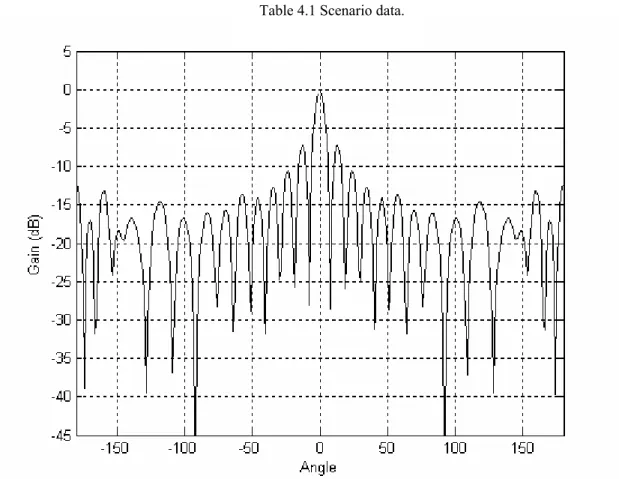
(9) Chapter 4 Results and Simulations In this chapter, we present the results obtained for the model proposed in chapter 3. The scenario is analyzed by varying some parameters like radiation pattern, mobile direction, beamwidth, srw and mobile position. Also we made simulations to determinate the behavior of the Doppler spectra when distances are involucrate in the radio link.. 4.1 Different Radiation Pattern This section deals with the results on PDS when four different radiation patterns are implemented at the BS, omnidirectional, sectorized, linear and circular array. We assume a mobile’s velocity of 54 km/h and a carrier frequency of 2 GHz; thus the maximum Doppler shift will be 100 Hz. To take into account the Macrocell scenario we defined D=1000 m and srw =100 m as was establish in [4] and a beamwidth for sectorized and smart antennas of BW=150 as shown Table 4.1. The radiation patterns of the linear and circular arrays are shown in Figures 4.1 and 4.2 respectively; it is easy to observe that the lateral lobes of the linear array are smaller than the lateral lobes of the circular array. For instance in the case of an omnidirectional antenna all the scatters contribute to the PDS (Clarke´s Model), while for a sectorized antenna all the scatters outside the antenna view are cut off considering only those scatters that are illuminated, in the case of smart antenna, the scatters contribution to PDS will be affected by the antenna gain in the corresponding AOA at the BS, see Figure 4.3.. 23.

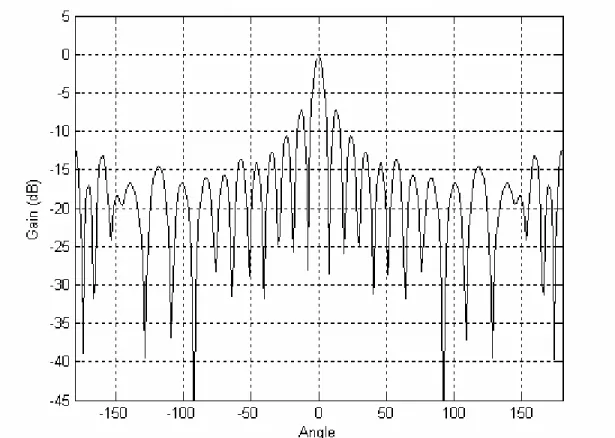
(10) Chapter 4. Results and Simulations. The scatters in the region A1 cause a positive Doppler shift and those in region A2 cause a negative Doppler shift. fc velocity fm D srw BW. 2 GHz 54 km/h 100 Hz 1000 m 100 m 150 Table 4.1 Scenario data.. Figure 4.1 Linear radiation pattern BW=150.. Two mobile directions with respect to LoS are considering θ v = 180 0 and θ v = 90 0 , see Figures 4.3a and 4.3b respectively. When θ v = 180 0 , we can see in Figure 4.4 that the contribution to the different Doppler frequencies of the smart antennas is lower than the contribution made by the omnidirectional and sectorized antennas, because the scatterers are take in to account in a different way due the gain G (θ b ) and affect mainly to the large Doppler shift.. 24.

(11) Chapter 4. Results and Simulations. Figure 4.2 Circular radiation pattern BW=150.. a). 25.

(12) Chapter 4. Results and Simulations. b) Figure 4.3 Scatterers illuminated by a sectorized and smart antennas. a) Toward BS b) Perpendicular BS. We also note that the negative Doppler shift is lightly greater because there are more scatteerrs illuminated at the right side of the MS and the direction θ v is towards the BS what means it moves away of those scatterers (negative Doppler frequencies).. Figure 4.4 Macrocell Power Dopler Spectrum with θv=1800.. 26.

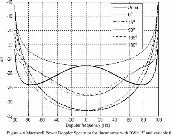
(13) Chapter 4. Results and Simulations. Now, we observe the behavior of the PDS when the direction of motion of the MS is. θ v = 90 0 Fig. 4.5. It is noted that when the MS is traveling perpendicularly to the direct path the smart antennas give higher spectral content near to 0 Hz than for the lateral frequencies due to the fact that the principal gain is concentrated in angles close to LoS. With this direction asymmetric between the positive and negative Doppler frequencies does not exist, because on the average the scatterers located upside the MS are the same as those located downside. It is being noted that the behavior of the PDS for linear and circular arrays is almost the same just with a little difference caused by the lateral lobes, as was shown in Figures 4.1 and 4.2.. 4.2 Different Mobile Direction In order to observe the gradual change of the PDS when the direction of motion of the MS θ v varies, we utilize the scenario of the previous section employing linear and circular arrays at the BS and changing the direction of motion θ v as it is shown in the figure 4.6 and 4.7. It can be observed that the PDS for θ v = 0 0 and for θ v = 180 0 are mirrored images. The same effect occurs for 450 and 1350.. Figure 4.5 Macrocell Power Doppler Spectrum with θv=900.. 27.

(14) Chapter 4. Results and Simulations. Figure 4.6 Macrocell Power Doppler Spectrum for linear array with BW=150 and variable θv.. Figure 4.7 Macrocell Power Doppler Spectrum for circular array with BW=150 and variable θv.. 28.

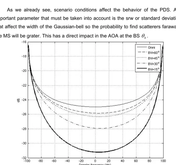
(15) Chapter 4. Results and Simulations. 4.3 Different Beamwidth The beamwidth for this thesis was taken to be the angular spacing of the two nulls around the main lobe gain. In order to show the effect for varying the BW on the PDS, results for linear array are presented in Figures 4.8 and 4.9 for travel directions and. θ v = 180 0 and θ v = 90 0 . The Doppler spread decreases significantly as the BW of the antenna reduces. As the BW reduces, the antenna is able to mitigate multipath components with large AOAs. It also can be observed that as the BW becomes wider the PDS tends towards the U-shaped Clarke’s Model (omnidirectional antenna). The results with circular arrays are quite similar, as we saw for the other sections.. 4.4 Different Scattering Region Width As we already see, scenario conditions affect the behavior of the PDS. Another important parameter that must be taken into account is the srw or standard deviation (σ), that affect the width of the Gaussian-bell so the probability to find scatterers faraway from the MS will be grater. This has a direct impact in the AOA at the BS θ b .. Figure 4.8 Macrocell Power Doppler Spectrum for linear array with θv=1800 and variable BW.. 29.

(16) Chapter 4. Results and Simulations. ( ). Therefore, the gains G θ bi separated by the principal lobe will have a greater contribution on the PDS.. Figure 4.9 Macrocell Power Doppler Spectrum for linear array with θv=900 and variable BW.. The Figures 4.10 and 4.11 present the results when a linear array is implemented at the BS with a BW=150 and varying the srw for mobile direction θ v = 180 0 and. θ v = 90 0 respectively.. 30.

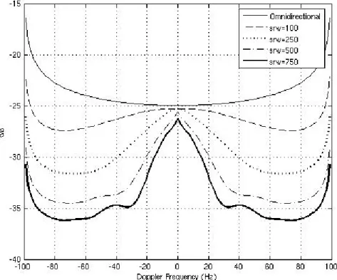
(17) Chapter 4. Results and Simulations. Figure 4.10 Macrocell Power Doppler Spectrum for linear array with θv=1800, BW=150 and variable srw.. Figure 4.11 Macrocell Power Doppler Spectrum for linear array with θv=900, BW=150 and variable srw.. 31.

(18) Chapter 4. Results and Simulations. Next, in Figures 4.12 and 4.13 shown the effects when a circular array is now utilized at the BS.. Figure 4.12 Macrocell Power Doppler Spectrum for circular array with θv=1800, BW=150 and variable srw.. Figure 4.13 Macrocell Power Doppler Spectrum for circular array with θv=900, BW=150 and variable srw.. 32.

(19) Chapter 4. Results and Simulations. By observing carefully the past figures, we can note that the shape of the PDS stay constant, when θ v = 180 0 the negative Doppler frequencies are favored and when θ v = 90 0 the model predicts higher spectral power near to the central frequency (0 Hz). The differences are caused by the lateral lobes that have major participation due to the increment in the probability of having a scatterer faraway from the MS.. 4.5 Different Mobile Position A common convention has been to take the straight line passing through the BS and MS as a coordinate axis with origin at the BS as we saw in Figure 2.7 in chapter 2. This convention is useful with omni and sectorized antennas as well as circular arrays near symmetric receiving pattern respect to the BS direction. It has also been customary to consider only those scatterers to the right side of the BS due equation (3.1). However, in the case of linear arrays the beam presents a specular pattern with respect to the antenna axis (see Figure 4.13). In this case the effective scatteres will take place in a ± π / 2 window centered at the mobile direction. So, the main and specular lobes will affect the Doppler spectra.. Figure 4.14 Linear radiation pattern with the main lobe at 450.. 33.

(20) Chapter 4. Results and Simulations. Figures 4.15 shows the performance of the linear array when it is steering at different mobile positions. We consider a beamwidth at the BS of 150 in the main lobe. To point out the effect of the specular lobe we choose θ v = 90 0 because the behavior is symmetric between the positive and negative Doppler shift, as we already saw in the past sections. Observing the figure we note an asymmetry caused by the specular lobe, this is obvious due to the fact the scatterers localized downside the direct path will be affected by lower gains than the scatterers localized upside the direct path where the specular lobe is located.. Figure 4.15 Macrocell Power Doppler Spectrum for different angles in the main lobe linear array BW=150 θv=900.. 4.6 Simulations of Distances Simulation is a great tool to evaluate different kinds of problems in communications systems, when you do not have the analytical answer or when mathematics become so complex that is not recommended go on. However you can generate the scenario through computer programs or software and set up some parameters to obtain an outcome, certainly not the right exact but we will get some clues that guide our research.. 34.

(21) Chapter 4. Results and Simulations. The previous sections deal with the PDS without taking in to account the distance traveled by every multipath. There is a loss of power due to the separation between the transmitter and the receiver. This section presents simulations in order to obtain the power contribution of the different multipath to the Doppler frequencies.. 4.6.1 Propagation Model Propagation models have traditionally focused on predicting the average received signal strength at a given distance from the transmitter. A common large scale propagation model is. Pr (d ) = Pt (d ) −α. (4.1). where Pt is the transmitted power, Pr (d ) is the received power which is a function of the transmitter-receiver separation, d is the transmitter-receiver separation in meters and finally α is the path-loss exponent settled in 3 like an urban areas. As we already saw in section 2.3, in GSDM there are two distances that intervene in the propagation of every multipath component, rm the distance between the MS and the scatterer and rb that is the distance between the scatterer and the BS, so using (4.1) we obtain. Pr = Pt (rm + 1) −α (rb + 1) −α. (4.2). we add unity just in case the distance happens to be zero.. 4.6.2 Simulation of the GSDM In order to create a Gaussian Scatter Density Model, we generate scatterers points using the joint pdf (2.9) set the distance between the MS and BS to D=1000 m and the scattering region width or standard deviation srw=100 m. Then a (x,y) position respect to the MS is given by the pdf, finally using the Pitagoras theorem and cosine-law we found. rm , rb , θ m and θ b of every scatterer generated.. 35.

(22) Chapter 4. Results and Simulations. First we compare our simulation with the Clarke´s model see Figure 4.16, without adding the propagation loss due to the distances. When the GSDM is used in a scenario that employs omnidirectional antenna the results must tend to the Clarke’s model because the marginal pdf of θ m is a uniform distribution between 0 and 2π.. Figure 4.16 Comparison between the Clarke’s Model and the simulation.. We can see that the behavior of the simulation is almost the Clarke’s Model and only 200000 scatterers points were simulated. Now, we add the propagation loss due the distances, see Figure 4.17. Also with 200000 scatterers point. Observing the Figure 4.17, we can not conclude anything because there is no way to characterized a behavior, so a new simulation is made using 6 millons of scatterers points, as we see in Figure 4.18. In this figure we note a U-shape behavior like the Clarke´s Model, but can not assure any conclusions.. 4.6.3 Scatterers Circle In order to obtain a more clearing explanation of the behavior of the PDS when the propagation loss is included we decided to divided the scenario in circles of radius rm, as shown in Figure 4.19. First we fix the radius rm and generate scatterers with a uniform. 36.

(23) Chapter 4. Results and Simulations. distribution between 0 and 2π. This obviously tends to the Clarke´s model if the propagation loss is not included as we see in Figure 4.20 here we generate 100000 scatterers points.. Figure 4.17 Simulation of distances using 200000 scatterers points.. 37.

(24) Chapter 4. Results and Simulations. Figure 4.18 Simulation of distances using 6 millions of scatterers points.. In order to diminish the time of simulation we quantize the circle (0 a 2π) in to 20000 parts and generate a scatterer in that angle, obtaining better results as we can observe in Figure 4.21.. Figure 4.19 Scenario divided in circles of radio rm.. 38.

(25) Chapter 4. Results and Simulations. Figure 4.20 Comparison between Clarke´s model and the simulation 100000 scatterers points around a circle of radius rm.. Figure 4.21 Circle quantized simulation.. 39.

(26) Chapter 4. Results and Simulations. Figure 4.22 show the PDS behavior when the propagation loss is taking in to account and different radiuses are implemented.. Figure 4.22 Circle quantized simulation including propagation loss for different rm.. It is easy to observe that the circle with the larger radius experiments more propagation loss. This experiment is just one of the steps we need to establish. When the scenario is divided into k circles, is affected the PDS by the probability of the distance rm. The marginal pdf of the distance rm is given by a Raleygh distribution. f rm (rm ) =. ⎛ r ⎞ exp⎜ − m2 ⎟ σ ⎝ σ ⎠ rm. 2. (4.3). and the probably of being a distance rm from the MS is given by r +1. r. P{rm = r} =. ∫f. rm. (rm )drm +. r −1. ∫f r. 2. 40. rm. (rm )drm (4.4).

(27) Chapter 4. Results and Simulations. Establishing a Gaussian scenario with D=1000 m and srw=100 m, the figure 4.23 shows the PDS when the procedure early explained is used.. Figure 4.23 PDS with a Raleygh distribution of the distances.. Figure 4.24 Normalized PDS with Raleygh distribution of the distances and normalized Clarke’s Model.. 41.

(28) Chapter 4. Results and Simulations. Now, we can assured that the model tends to the U-shaped like in the Clarke´s model. In order to make a better comparision we normalize the results obtained and the results for the Clarke model, as can be seen in Figure 4.24. Observe that the differences are minimal.. 42.

(29) Chapter 2 Basic Concepts in Wireless Communications In a wireless system, a signal transmitted through the channel interacts with the environment in a very complex way. There are reflections from large objects, diffraction of the electromagnetic waves around the objects and signal scattering. The result of these complex interactions is the presence of many signal components, or multipath signals, at the receiver. A multipath environment with two MS is shown in Figure 2.1. Each signal component experiences a different multipath environment which determines the amplitude, carrier phase shift, time delay, direction of arrival and Doppler shift of each multipath for every mobile.. 2.1 Doppler Shift The Doppler shift is a change in frequency induced by the motion of the receiver. Depending on the direction of motion θ v of the MS relative to the BS and AOA at the MS. θ m , as it is seen in Figure 2.2, whether the component is a direct path or a multipath component. The Doppler frequency is given by [11]. υ i = f m cos(θ m − θ v ) i. where f m =. v. λ. fi < f m. (2.1). is the maximum Doppler shift, v is the mobile velocity and λ is the carrier. frequency wavelength. Equation (2.1) relates the Doppler shift to the mobile. 3.

(30) Chapter 2. Basic Concepts in Wireless Communications. velocity and the spatial angle between the direction of motion of the mobile and the direction of arrival of the wave. It can be see that if the mobile is moving toward the Scatterer. Scatterer Figure 2.1 Signals from two MS incident to BS in a multipath channel.. direction of arrival of the wave, the Doppler shift is positive, and if the mobile is moving away from the direction of arrival wave, the Doppler shift is negative see Appendix A. Multipaths components from a continuous wave signal that arrive from different directions contribute to Doppler spreading of the received signal, thus increasing the signal bandwidth [11]. Scatterer. Figure 2.2 MS traveling in a direction θv.. 4.

(31) Chapter 2. Basic Concepts in Wireless Communications. 2.2 Doppler Spectra and the Fading Envelope Consider a MS, traveling at speed v , which receiving a signal at a carrier f c . Because of multipath, several replicas of the transmitted signal arrive at the receiver. Each multipath replica of the received signal will experience a Doppler shift υ i due the motion of the user, equation (2.1). The baseband complex equivalent representation of the received signal at the mobile unit is L −1. r (t ) = E0 ∑ α i e j 2πυit. (2.2). i =0. where α i is the complex multipath amplitude for multipath component i . The power spectral density of the received signal is given by. Sr ( f ) =. [. lim 1 * E RT ( f ) RT ( f ) T → ∞ 2T. ]. (2.3). where RT ( f ) is the finite time Fourier transform of r (t ) . The power spectral density, which shows the spreading of the signal in the frequency domain due the motion of the MS is referred to as the Doppler spectrum. The finite time Fourier transform of r (t ) is. L −1 ⎛ L −1 ⎞ RT ( f ) = ∫ ⎜ E0 ∑ α i e j2πυit ⎟e 2πft dt = E0 ∑ α i ∫ e j2π (υi − f )t dt i =0 i =0 ⎠ −T ⎝ −T T. T. L −1. = E0 ∑ α iT i =0. sin (2π (υ i − f )T ) 2π (υ i − f )T. (2.4). Then, assuming that the magnitude of each multipath component, α i , is a constant we may express the Doppler spectrum as. Sr ( f ) =. lim 1 ⎡ 2 2 L −1 L −1 sin (2π (υ i − f )T ) sin (2π (υ j − f )T )⎤ E ⎢ E0 T ∑∑ α iα j * ⋅ ⎥ T → ∞ 2T ⎢⎣ 2π (υ i − f )T 2π (υ j − f )T ⎥⎦ i =0 j = 0 = fυ ( f ) ⋅. E02 4. L −1. ∑α i =0. 2 i. 5. = A02 fυ ( f ). (2.5).

(32) Chapter 2. Basic Concepts in Wireless Communications. where fυ (υ ) is the probability density function describing the distribution of the Doppler. We may use standard techniques for determining the distribution of a function of a random variable to find the pdf of υ i from the pdf of θ mi using (1) [5]. Thus. fυ (υ ) =. (. fθ m θ v + cos −1 (υ f m ) f m 1 − (υ f m ). 2. ) + f (θ θm. v. − cos −1 (υ f m ). ). f m 1 − (υ f m ). 2. υ < fm. (2.6). Using (2.5), the power spectral density of the received signal is. Sr ( f ) =. A02 fm 1− ( f fm ). 2. [ f (θ θm. v. ). (. + cos −1 ( f f m ) + fθ m θ v − cos −1 ( f f m ). )]. f < fm. (2.7). The traditional model where the AOA is uniformly distributed on [− π , π ], the Doppler spectrum takes on the expression presented by Clarke [6] [7]. Sr ( f ) =. A02. πf m 1 − ( f f m )2. f < fm. Clarke’s Doppler power spectrum is illustrated in Figure 2.3.. Figure 2.3 Clarke´s model for the Doppler power spectrum.. 6. (2.8).

(33) Chapter 2. Basic Concepts in Wireless Communications. 2.3 Channel models The spatial information from the different paths is necessary to develop the desired radiation pattern that improves the system response. This information represents the characteristics of arrival of each path (AOA, distance, delay). Certainly, a whole representation of all paths in a real environment will be very hard to produce. However, some models have been proposed in order to provide enough information about the channel. Among the most popular models we may find Lee’s Model, the Geometrically Based Single Bounce (GBSB) statistical channel models, Gaussian Wide-Sense Stationary Uncorrelated Scattering (GWSSUS) model and the Gaussian Scatter Density Model (GSDM) clearly illustrated in the next section, we will briefly present a light explanation of the rest. A deeper explanation of some models can be found in [13]. In Lee´s Model, scatterers are evenly spaced on a circular ring around the mobile, as shown in Figure 2.4. Each of the scatterers is represents the effect of many scatterers within the region. This model was originally used to predict the correlation between the signals received by two sensors as a function of the element spacing.. Figure 2.4 Lee´s Model.. Among the GBSB models, we find the geometrically based circular. This model assumes that the scatterers lie within a circle of radius Rm around the MS as seen in. 7.

(34) Chapter 2. Basic Concepts in Wireless Communications. Figure 2.5. It was originally proposed to derive theoretical results for the correlation observed between two antenna elements; it was also used to determinate the PDS with sectorized antenna [3].. Figure 2.5 Geometrical Based Circular Model.. In the GWSSUS model, the scatterers are grouped into clusters, as shown in Figure 2.6, where there are three clusters. By including multiple clusters, frequency-selective fading channels can be modeled. The problem with this model is that it does not indicate the number or location of the scattering clusters, and therefore requires some additional information.. Figure 2.6 GWSSUS Model.. 8.

(35) Chapter 2. Basic Concepts in Wireless Communications. It has been demonstrated by measures in outdoor and indoor environments and by simulations that the GSDM is the most realistic channel model [14] [15]. From a physical viewpoint it seems more reasonable to assume that the scatterer density gradually taper off with distance from the transmitting antenna as remote will in general have less contribution than close-in scatterers [1] .. 2.4 Gaussian Scatter Density Model The GSDM [1] [4], assumes that the scattering points are Gaussianly distributed centered at the MS location. The model assumes that the energy received by path passing through several scattering points is minor, so only one bounce traveling from the transmitter to the receiver is considering. For MS D units apart from the BS, see Figure 2.7, the scatterers location can be describe as. f xm , y m ( x m , y m ) =. ⎛ xm2 + y m2 ⎞ ⎟ ⎜⎜ − exp 2πσ 2 2σ 2 ⎟⎠ ⎝ 1. (2.9). when the MS location is taken as coordinates reference, the figure 2.8 shows the join pdf of the random variables xm and y m . If the coordinate’s origin is placed at BS, the scatterers will be distributed according to the join pdf (2.10) where σ is the measure srw related to the scatterers concentration around the mobile.. Figure 2.7 Gaussian scattering scenario.. 9.

(36) Chapter 2. Basic Concepts in Wireless Communications ⎛ ( xb − D) 2 + yb2 ⎞ ⎟⎟ f xb , yb ( xb , yb ) = exp⎜⎜ − 2 2πσ 2 2 σ ⎠ ⎝ 1. (2.10). Alternatively scatterers location can be described using polar coordinates (rb ,θ b ). and (rm ,θ m ) as seen from BS or MS respectively see Appendix B.. Figure 2.8 Joint pdf of the location of the scatterers.. So that the joint pdf in polar coordinates yields. f rm ,θ m (r m , θ m ) =. ⎛ rm2 ⎞ ⎟ ⎜⎜ − exp 2 ⎟ 2πσ 2 ⎝ 2σ ⎠ rm. (2.11). and the marginal pdf of the AOA θ b is. ⎛ − D 2 sin 2 (θ b ) ⎞ D cos(θ b ) ⎛ − D2 ⎞ 1 ⎛ − D cos(θ b ) ⎞ ⎟⎟ ⋅ ⎟ ⎜ ⋅ erfc⎜ exp⎜ + exp⎜⎜ fθb (θ b ) = ⎟ 2 ⎟ 2 2π 2σ 2σ ⎝ ⎠ ⎝ 2σ ⎠ ⎠ 2 2π σ ⎝ where erfc is know like complementary error function [1] [2].. 10. (2.12).

(37) Chapter 2. Basic Concepts in Wireless Communications. 2.5 Smart Antennas Smart antenna system is a combination of two technologies adaptive antenna and switched beam technology; adaptive antenna is an array of antennas which is able to change its antenna pattern dynamically to adjust to noise, interference and multipath. Adaptive array antennas can adjust their pattern to track portable users. Adaptive antennas are used to enhance received signals and may also be used to form beams for transmission. Switched beam systems use a number of fixed beams at an antenna site. The receiver selects the beam that provides the greatest signal enhancement and interference reduction [5]. Figure 2.9 shows a smart antenna with different lobes.. Figure 2.9 Smart antenna can form a different lobe or beam for each subscriber.. 2.5.1 Linear Array A linear array is the simplest model. In Figure 2.10 a uniformly spaced linear array is depicted with K identical isotropic elements, this mean that each element radiates radiates in all directions with the same power. Each element is label with a complex weight Vk with k=0, 1…, K-1, and the interelement spacing is denoted by d. If a plane wave impinges at the array with an angle θ with respect to the array normal, the waveform arrives at element K sooner than the element K-1, where the differential distance along two rays is. d sin(θ ) . By setting the phase of the signal at the origin arbitrarily to zero, the phase leads of the signal at element K relative to that at element 0 is κkd sin(θ ) , where κ =. λ = wavelength. 11. 2π. λ. and.

(38) Chapter 2. Basic Concepts in Wireless Communications. Figure 2.10 Uniformly spaced linear array.. Adding all the elements outputs together gives what is commonly referred to as array factor F K −1. F (θ ) = V0 + V1e jκd sin θ + V1e j 2κd sin θ + ... = ∑Vk e jκkd sin θ. (2.13). k =0. The array factor may be expressed in term of vector inner product. F (θ ) = V T υ. (2.14). where. V = [V0 V1 ... Vk −1 ]. T. is the weighting vector and. υ = [1 e jκd sin θ ... e j ( K −1)κd sin θ ]. T. 12.

(39) Chapter 2. Basic Concepts in Wireless Communications. is the array propagation vector, which contains the information about the origin of the signal. If the complex weight is. Vk = Ak e jkα. (2.15). where the phase of the k-th element precedes that of the (k-1)-th element by α , and the array factor becomes K −1. F (θ ) = ∑ Ak e j (κkd sin θ + kα ). (2.16). k =0. If α = −κd sin θ 0 , a maximum response of F (θ ) will result at the angle θ 0 , wich means that the main beam or lobe has been steered towards the wave source. An example of F (θ ) for a linear array is given in Figure 2.11, where the antenna beam is steered towards the antenna foresight [9].. Figure 2.11 Beam pattern of a linear array.. 13.

(40) Chapter 2. Basic Concepts in Wireless Communications. 2.5.2 Circular Array A circular array consisting of K identical isotropic elements uniformly arranged around a circle of radius R. Each element is label with a complex weight Vk with k=0, 1…, K-1. Since the K elements are arranged at an equal distance from one another around the circle, the azimuth angle of kth element is given by φ k = 2kπ / K . If a plane wave impinges upon the array in the direction (θ , φ ) , as shown in Figure 2.12, the relative phase at the kth element with respect to the center of the array is given by. β k = −κR cos(φ − φk ) sin θ. (2.17). Figure 2.12 Circular array with equally spaced K elements.. If follows that the array factor for a circular array with K equally spaced elements is given as K −1. F (φ ,θ ) = ∑ Ak e j [α k −κR cos(φ −φk ) sin θ ] k =0. 14. (2.18).

(41) Chapter 2 where Ak e. Basic Concepts in Wireless Communications jα k. denotes the complex weight for the kth element. In order to have the main. beam directed at the angle (φ0 ,θ 0 ) in space, the phase of the weight for the kth element can be chosen as. α k = κR cos(φ0 − θ 0 ) sin θ 0 An example of the three-dimensional pattern of a circular array is shown in Figure 2.13. In many applications, such as BS antennas, the pattern in the θ =. π 2. plane is of. interest. In this case the array factor is giving by K −1. F (φ ) = ∑ Ak e j [α k −κR cos(φ −φk ) ]. (2.19). k =0. z. y. x. Figure 2.13 Three-dimensional beam pattern of a circular array.. One of the inherent characteristics of a circular array is the presence of high sidelobe levels in the beam pattern [9] [12].. 15.

(42) Chapter 5 Conclusion and Future Work In the present chapter, we include the general conclusions of this thesis, and we also include certain topics for further work in the same line of research in order to continue with the work on PDS and smart antennas.. 5.1 Conclusions In this work we have proposed a method that tries to characterize the behavior of the PDS when smart antennas are deployed at the BS. In addition, we have made the analysis of the method in certain wireless communications scenarios that present different characteristics about beampattern, beamwidth, mobile direction, scattering region width and mobile position, in order to evaluate the PDS. The results presented in Chapter 4 reveal to us that both lineal and circular arrays have almost the same performance when they are steering to 00 and the PDS present less spread than when omnidirectional and sectorized antenna are being used at the BS. In addition we observe the undesired effect of the specular lobe in lineal array that affect the shape of the PDS when we take a different position of the MS. We can conclude that the model developed gives a good approximation of the comportment of the Doppler spectra when arrays of antennas are employing, rested importance to the fact that we only made a discretization of the scenario. Observing the results presented by the simulation of distances, we take the risk to say we found an alternative to the analytical way to characterize this phenomenon.. 43.

(43) Chapter 5. Conclusions and Future Work. 5.2 Future Work According to the work done in this thesis, the following topics are suggested for further research. •. Analytical results when distances are taking in to account in GSDM environment, in order to evaluate the PDS.. •. Simulation of the GSDM environment without take into account the distances and adding the gains of the smart antennas and compare with the analytical results.. •. Simulation of the distances in a GSDM environment adding the gains of the smart antennas.. 44.

(44) Bibliography [1] Janaswamy R., “Angle and time of arrival statistics for the Gaussian scatter density model”, IEEE Trans. On Wireless Communications vol 1, pp. 488-497, 2002.. [2] Lopez C. A., Covarrubias D. H., “Statistical cellular gaussian scatter density Channel model employing a directional antenna for mobile environments”, International Journal of Electronics and communication (AEU) vol 59, pp. 195199, April, 2005.. [3] Petrus P., Reed J., Rappaport T. S., “Geometrical-based statistical macrocell channel model for mobile environments”, IEEE Trans. On Comms. vol 50, pp. 495-502, 2002.. [4] Lotter M. P., Van Rooyen, P., “Modeling Spatial aspects of cellular CDMA/SDMA systems”, IEEE Communications Letters vol 3, pp. 128-131, 1999.. [5] Liberti Jr., Rappaport T. S. , “Smart antennas for wireless communications: IS95 and third generation CDMA applications”, New York: Prentice Hall, 1999.. [6] Clarke R. H., “A statistical theory of mobile-radio reception”, The bell system technical Journal vol 1, pp. 957-1000, 1968.. [7] Jakes W. C., “Microwave mobile communications”, IEEE Communications. Society, 1974.. [8] Crohn I., Bonek E., “Modeling of. intersymbol - interference in a Rayleigh fast. fading channel with typical delay profile”, IEEE Trans Veh. Technol pp. 438447, 1992.. 45.

(45) Bibliography. [9] Litva J., Kwong-Yeung T., “Digital Beamforming in Wireless Communications”, Artech House, 1996.. [10] Liberti J., “Measuring and Modeling Spatial Radio Channels for Smart Antenna. Systems”,. IEEE. International. Symposium. of. Antennas. and. Propagation Society, Vol. 2, pp. 635 -638, June 1998. [11] Rappaport, T. S. , “Wireless Communications Principles and Practice”, Prentice Hall, Second Edition, 2002.. [12] Sid-Ahmed M. A., “Two’s-complement systolic array multiplier with applications to dsp hardware”, Int. J. Electronics, vol 66, pp. 507-518, 1989. [13] Ertel B., Cardieri K., Rappaport T. S. , “Overview of spatial Channel Models for Antenna array Communications System”. IEEE Personal Communications Magazine, Vol. 5, No. 1, February, 1998. [14] Spencer Q. H., Jeffs B. D., Jensen M. A., Swindlehurst A. L., “Modeling the statistical time and angle of arrival characteristics of an indoor multipath channel”, IEEE J. Select. Areas. Commun., vol. 18, pp. 347–360, Mar. 2000.. [15] Pedersen K. I., Mogensen P. E., Fleury B. H., “Power azimuth spectrum in outdoor environments”, IEEE Electron. Lett., vol. 33, pp.1583–1584, Aug. 1987.. 46.

(46) Appendix A Positive and Negative Doppler Shift This appendix briefly describes the way to obtain the Doppler shift, given by Equation (2.1) in Section 2.1. Consider the scenario presented in Figure A.1, the MS direction is 1800 towards the BS but away from the scatterers that generate multipahts increasing the negative Doppler frequencies.. Figure A.1 MS move away from the scatterers.. Now suppose that the MS moves towards the scatterers as we see in Figure A.2., The multipaths contribute to the positive Doppler frequencies. When the direction of motion of the MS changes, the contribution to the positive and negative Doppler frequencies changes too. Observe Figure A.3.. 47.

(47) Appendix A. Figure A.2 MS move toward the scatterers.. The direction of the MS is 900, we observe that the mobile is moving away from one scatterer but comes near to an other, then we affect both positive and negative Doppler frequencies.. Figure A.3 MS direction motion 900.. 48.

(48) Appendix B Polar Transformation and Marginal PDF This Appendix deals with the procedure of converting rectangular coordinates in to polar coordinates and the way to obtain the marginal pdf. The joint pdf of two Gaussian random variables is given by (2.9) in section 2.4, we can deduce from Figure 2.4 that. xm = rm cos(θ m ). (B.1). y m = rm sin (θ m ). (B.2). and using the jacobian obtain. ⎡ ∂x m ⎢ ∂r J (rm , θ m ) = ⎢ m ⎢ ∂y m ⎢⎣ ∂rm. ∂x m ⎤ ∂θ m ⎥ ⎡cos(θ m ) − rb sin (θ m )⎤ ⎥ = ∂x ⎥ ⎢⎣ sin(θ m ) rb cos(θ m ) ⎥⎦ ∂θ m ⎥⎦. (. ). J (rm , θ m ) = rm cos 2 (θ m ) + sin 2 (θ m ) = rm. in such a way that the joint pdf in polar coordinates yields. f rm ,θ m (r m , θ m ) =. ⎛ rm2 ⎞ ⎟ ⎜⎜ − exp 2 ⎟ 2πσ 2 ⎝ 2σ ⎠ rm. 49. (B.3).

(49) Appendix B. using the same method we obtain the joint pdf of the scatterers position when the coordinates origin is placed at the BS.. ⎛ (rb cos(θ b ) − D )2 − (rb sin(θ b ) )2 ⎞ ⎟ f rb ,θb (r b , θ b ) = exp⎜⎜ − 2 ⎟ σ 2πσ 2 2 ⎝ ⎠ rb. (B.4). In order to get the marginal pdf of the AOA θ b at the BS, we must integrate the variable rb over all the existing range. Rearranging and integrating (B.4) yields ∞. (. ). ⎛ rb2 − 2 Drb cos(θ b ) + D 2 ⎞ ⎟⎟ dr ⎜⎜ − exp 2σ 2 2πσ 2 ⎠ ⎝ 0 ∞ 2 2 ⎛ (rb − D cos(θ b ) )2 ⎞ ⎛ − D sin (θ b ) ⎞ rb ⎜ ⎟ dr ⎟⎟ ∫ = exp⎜⎜ exp⎜ − 2 2 2 ⎟ σ πσ σ 2 2 2 ⎠0 ⎝ ⎝ ⎠ Changing the variable r − D cos(θ b ) x= b rb = 2 xσ + D cos(θ b ) 2σ dr dx = drb = dx 2σ 2σ Limits − D cos(θ b ) rb = 0 x= 2σ rb = ∞ x=∞ fθb (θ b ) = ∫. rb. ⎛ − D 2 sin 2 (θ b ) ⎞ ∞ 2 xσ + D cos(θ b ) ⎟⎟ ∫ fθb (θ b ) = exp⎜⎜ exp − x 2 dx 2σ 2 2 2σ 2πσ ⎠ − D cos (θb ) ⎝. (. ). 2σ. ⎤ ⎛ − D sin (θ b ) ⎞ ⎡ 1 D cos(θ b ) 2 2 2 ⎟ x x dx x dx exp exp − + − = exp⎜⎜ ⎥ ⎢ ∫ 2πσ ⎟ ∫π 2σ 2 ⎠⎣ ⎝ ⎦ ∞ 2 2 2 ⎛ − D sin (θ b ) ⎞ D cos(θ b ) ⎛−D ⎞ 1 ⎟⎟ ⋅ ⎟ + exp⎜⎜ exp x 2 dx exp⎜⎜ = 2 2 ⎟ ∫ 2σ 2π 2πσ − D cos (θb ) ⎝ 2σ ⎠ ⎠ ⎝ 2. 2. (. ). (. ). ( ). 2σ. =. ⎛ − D 2 sin 2 (θ b ) ⎞ D cos(θ b ) ⎛ − D2 ⎞ 1 ⎛ − D cos(θ b ) ⎞ ⎟⎟ ⋅ ⎜⎜ ⎟ exp⎜⎜ exp ⋅ erfc⎜ + ⎟ 2 ⎟ 2 2π 2σ 2σ ⎠ ⎝ ⎝ 2σ ⎠ ⎠ 2 2π σ ⎝. 50. (B.5).

(50) Appendix B. we know that erfc( z ) =. ∞. exp(− t )dt π ∫. 2. 2. z. 51.

(51) Contents List of Figures………...................................................................................................iii List of Tables……..........................................................................................................v List of Acronyms…….................................................................................................vii Chapter 1 Introduction.................................................................................................1 1.1 Objective……………...................................................................................................2 1.2 Justification.................................................................................................................2 1.3 Organization……….....................................................................................................3. Chapter 2 Basic Concepts in Wireless Communications..............................3 2.1 Doppler Shift...............................................................................................................3 2.2 Doppler Spectra and the Fading Envelope.................................................................4 2.3 Channel Models………………….................................................................................7 2.4 Gaussian Scatter Density Model.................................................................................9 2.5 Smart Antennas........................................................................................................11 2.5.1 Lineal Array........................................................................................................11 2.5.2 Circular Array.....................................................................................................13. Chapter 3 Model Description……...........................................................................17 3.1 Classes of antennas..................................................................................................17 3.2 AOA…………….........................................................................................................18 3.3 PDS…………….........................................................................................................22. Chapter 4 Results and Simulation........................................................................23 4.1 Different Radiation Pattern........................................................................................23 4.2 Different Mobile Direction..........................................................................................27 4.3 Different Beamwidth..................................................................................................29 4.4 Different Scattering Region Width.............................................................................29 4.5 Different Mobile Position………….............................................................................33 4.6 Simulations of distances………….............................................................................34. i.

(52) 4.6.1 Propagation Model.............................................................................................35 4.6.2 Simulation of the GSDM.....................................................................................35 4.6.3 Scatterers Circle.................................................................................................36. Chapter 5 Conclusions and Future Work .........................................................43 5.1 Conclusions..............................................................................................................43 5.2 Future work...............................................................................................................44. Bibliography ………………………………………............................................................45 Appendix A ……………………………………….............................................................47 Appendix B ……………………………………….............................................................49. ii.

(53) List of Figures 2.1 Signals from two MS incident to BS in a multipath channel............................................4 2.2 MS traveling in a direction θv...........................................................................................4 2.3 Clarke´s model for the Doppler power spectrum............................................................6 2.4 Lee´s Model....................................................................................................................7 2.5 Geometrical Based Circular Model.................................................................................8 2.6 GWSSUS Model.............................................................................................................8 2.7 Gaussian scattering scenario..........................................................................................9 2.8 Joint pdf of the location of the scatters.........................................................................10 2.9 Smart antenna can form a different lobe or beam for each subscriber.........................11 2.10 Uniformly spaced linear array.....................................................................................12 2.11 Beam pattern of a linear array.....................................................................................13 2.12 Circular array with equally spaced K elements...........................................................14 2.13 Three-dimensional beam pattern of a circular array...................................................15 3.1 Different beam patterns steering 00..............................................................................18 3.2 Marginal pdf of the AOA at the BS θ b when D=1000 m and srw=750 m......................19 3.3 Scenario divided in sectors of angular width ∆.............................................................20 3.4 Scattering boundary region...........................................................................................21 4.1 Linear radiation pattern BW=150...................................................................................24 4.2 Circular radiation pattern BW=150………………………………………………………….25 4.3 Scatterers illuminated by a sectorized and smart antennas ………………………….....26 4.4 Macrocell Power Dopler Spectrum with θv=1800...........................................................26 4.5 Macrocell Power Doppler Spectrum with θv=900...........................................................27 4.6 Macrocell Power Doppler Spectrum for linear array with BW=150 and variable θv.......28 4.7 Macrocell Power Doppler Spectrum for circular array with BW=150 and variable θv....28 4.8 Macrocell Power Doppler Spectrum for linear array with θv=1800 and variable BW.....29 4.9 Macrocell Power Doppler Spectrum for linear array with θv=900 and variable BW...... 30 4.10 Macrocell Power Doppler Spectrum for linear array with θv=1800, BW=150 and variable srw.........................................................................................................................31 4.11 Macrocell Power Doppler Spectrum for linear array with θv=900, BW=150 and variable srw......................................................................................................................................31. iii.

(54) 4.12 Macrocell Power Doppler Spectrum for circular array with θv=1800, BW=150 and variable srw………………………........................................................................................32 4.13 Macrocell Power Doppler Spectrum for circular array with θv=900, BW=150 and variable srw.........................................................................................................................32 4.14 Linear radiation pattern with the main lobe at 450.......................................................33 4.15 Macrocell Power Doppler Spectrum for different angles in the main lobe lineal array BW=150 θv=900...................................................................................................................34 4.16 Comparison between the Clarke’s Model and the simulation.....................................36 4.17 Simulation of distances using 200000 scatters points................................................37 4.18 Simulation of distances using 6 millions of scatters points.........................................38 4.19 Scenario divided in circles of radio rm.........................................................................38 4.20 Comparison between Clarke´s model and the simulation 100000 scatters points around a circle of radius rm..................................................................................................39 4.21 Circle quantized simulation.........................................................................................39 4.22. Circle. quantized. simulation. including. propagation. loss. for. different. rm.........................................................................................................................................40 4.23 PDS with Raleygh distribution of the distances...........................................................41 4.24 Normalized PDS with Raleygh distribution of the distances and normalized Clarke’s Model..................................................................................................................................41. iv.

(55) List of Acronyms PDS. Power Doppler Spectrum. GSDM. Gaussian Scattering Density Model. BS. Base Station. MS. Mobile Station. AOA. Angle of Arrival. TOA. Time of Arrival. LCR. Level Crossing Rate. vii.

(56) List of Tables 4.1 Scenario data ...............................................................................................................24. v.

(57) vi.

(58) INSTITUTO TECNOLOGICO Y DE ESTUDIOS SUPERIORES DE MONTERREY CAMPUS MONTERREY PROGRAMA DE GRADUADOS DE LA DIVISION DE TECNOLOGIAS DE INFORMACION Y ELECTRONICA. Statistical Cellular Scatter Density Model (GSDM) Employing Smart Antennas for Macrocell Environments. THESIS Presented as a partial fulfillment of the requirements for the degree of. Master of Science in Electronic Engineering Major in Telecommunications. Ing. Jesús Mario Castrellón Rubio. Monterrey, N.L. December 2005.

(59) Instituto Tecnológico y de Estudios Superiores de Monterrey Campus Monterrey. División de Tecnologías de Información y Electrónica Programa de Graduados The members of the thesis committee recommended the acceptance of the thesis of Jesús Mario Castrellón Rubio as a partial fulfillment of the requirements for the degree of Master of Science in:. Electronic Engineering Major in Telecommunications THESIS COMMITTEE. David Muñoz Rodríguez, Ph.D. Advisor. César Vargas Rosales, Ph.D. Synodal. José Ramón Rodríguez Cruz, Ph.D. Synodal. Approved. David Garza Salazar, Ph.D. Director of the Graduate Program. December 2005.

(60) To god, he always takes care of me To my parents, Marisela and Jesús, my brothers, Carlos and Alberto and my grandma Jesusita for all their love Especially to my mom, she always believes in me To my girlfriend Wendy for be my inspiration To my advisor Dr. David Muñoz for be my guide.

(61) Statistical Cellular Scatter Density Model (GSDM) Employing Smart Antennas for Macrocell Environments Ing. Jesús Mario Castrellón Rubio Instituto Tecnológico y de Estudios Superiores de Monterrey, 2005. Abstract One way to evaluate the behavior of radio links is through Power Doppler Spectrum. However, under different channel models, the PDS change. This work presents an analysis of the effect on the PDS when smart antennas are deployed at the Base Station. The statistical Gaussian Scatter Density Model was the channel model used in the investigation. Two kinds of smart antennas were employed, linear and circular arrays. Omnidirectional and sectorized antennas were also included as a reference. As a result, we characterize the behavior of the PDS under different scenarios and compare with those for omnidirectional and sectorized antenna..

(62) Statistical Cellular Scatter Density Model (GSDM) Employing Smart Antennas for Macrocell Environments Ing. Jesús Mario Castrellón Rubio Instituto Tecnológico y de Estudios Superiores de Monterrey, 2005. Resumen Una manera de evaluar el comportamiento de los enlaces de radio es mediante el Espectro Doppler de Potencia. Sin embargo bajo distintos modelos de canal el Espectro Doppler cambia. Esta investigación analiza el Espectro Doppler cuando se utilizan antenas inteligentes en la estación base. El modelo de canal para dispersores en forma gaussiana es el usado en el desarrollo de la tesis. Dos clases de antenas inteligentes fueron empleados, arreglos lineares y arreglos circulares. El estudio del fenómeno en antenas omnidireccionales y sectorizadas fue como referencia. Como resultado final obtenemos una caracterización del comportamiento del Espectro Doppler, bajo distintos escenarios los cuales se comparan con los resultados para antenas omnidireccionales y sectorizadas..

(63)