Modelling of the dynamics of agroecological soil management and diet in the MEDEAS model framework

Texto completo

(1)UNIVERSITY OF VALLADOLID SCHOOL OF INDUSTRIAL ENGINEERINGS International Semester Program – Spring 2018. FINAL PROJECT. Modelling of the dynamics of agroecological soil management and diet in the MEDEAS model framework Author Doan, Trung Hieu Tutor Mediavilla, Margarita. Valladolid, June 2018..

(2) Table of contents. 1.. Introduction and objectives ................................................................................ 1. 2.. Method - System dynamics ................................................................................. 4. 3.. 2.1.. Introduction ................................................................................................... 4. 2.2.. The modelling process .................................................................................. 5. 2.3.. Several basic concepts in System dynamics ................................................ 7. 2.3.1.. Casual diagram ...................................................................................... 7. 2.3.2.. Feedback loops ....................................................................................... 7. 2.3.3.. Stocks and flows ..................................................................................... 9. Description of the model.................................................................................... 11 3.1.. 3.1.1.. Casual diagram .................................................................................... 12. 3.1.2.. Assumptions and model boundaries .................................................. 12. 3.2.. Forrester stock-flow diagram and description of variables .................... 14. 3.2.1.. Historical cropland .............................................................................. 15. 3.2.2.. Historical values and extrapolation of yield ...................................... 19. 3.2.3.. Transition of global diets and its impact ........................................... 22. 3.3. 4.. Overview of the model ................................................................................ 11. Scenarios of diets ......................................................................................... 25. Result and discussions ....................................................................................... 28 4.1.. Simulation result without peak oil effect .................................................. 28. 4.2.. Simulation result with peak oil effect ........................................................ 29. 4.3.. Limitations and implications of the model ............................................... 31. 4.3.1.. Limitations of the model ..................................................................... 31. 4.3.2.. Implications of the result .................................................................... 31. REFERENCES .......................................................................................................... 34.

(3) List of Figures and Tables Figure 1: The modelling process (Sterman, 2000) ........................................................ 6 Figure 2: Positive and negative casual links .................................................................. 7 Figure 3: Example of a stabilizing loop and a reinforcing one ...................................... 8 Figure 4: Graphs representing the behaviors of models having two kinds of loops (Martín, 2006) ................................................................................................................ 8 Figure 5: Hydraulic metaphor and the Forrester diagram (Sterman, 2000)................... 9 Figure 6: Casual diagram of the model ........................................................................ 12 Figure 7: Forrester stock-flow diagram of the model .................................................. 15 Figure 8: Stock-flow diagram of historical cropland ................................................... 16 Figure 9: Historical values of cropland, by each crop ................................................. 18 Figure 10: Calculation of land available for agricultural production .......................... 19 Figure 11: Stock-flow diagram of yield including the extrapolation and peak-oil effect ..................................................................................................................................... 19 Figure 12: Linear trend-line and extrapolation equation of cereals’ yield .................. 20 Figure 13: Crop production yield - with and without peak oil effect .......................... 22 Figure 15: Impact of dietary changes on demand for agricultural land ....................... 23 Figure 16: Crop production and land use by each diet (Stehfest et al., 2009) ............. 25 Figure 17: Land demand for food production by each diet - BAU.............................. 28 Figure 18: Land demand for food production by each diet – Peak oil effect .............. 30. Table 1: Adoption of dietary scenarios of Stehfest et al., 2009 into this model .......... 25 Table 2: Annual crop demand per capita (kg/person) for each diet ........................... 26 Table 3: Annual grassland per capita, by each diet (ha/person) .................................. 27 Table 4: Total land needed by each diet in 2050 - BAU ............................................. 29 Table 5: Total land needed by each diet in 2050 - Peak oil effect ............................... 31.

(4) 1.. Introduction and objectives. Food security is projected to be a major problem for mankind. Producing food for around 9 billion people by 2050 is certainly going to be challenging for the global agricultural sector (Diouf, 2009; United Nations Department of Economic and Social Affairs Population Division, 2017). Along with population growth, substantial income growth and urbanization, as well as the associated shifts in diet structures towards more nutritious and higher quality foods, is projected to result in almost the doubling of demand for food, feed and fibre (Diouf, 2009). As a consequence, agricultural production is required to soar. In fact, based on FAOSTAT 1, ever since the 1960s, an increase in both yield and cropland has been experienced, resulting in the overall rise in production. Either one of these factors is expected to keep on growing in order for the agricultural sector to feed the global populace and keep up with the trending dietary change.. However, the need for land dedicated to other purposes has increased significantly, exerting enormous pressures on allocation of agricultural land use. Firstly, the transition towards renewable energy has intensified the competition for land globally (Capellán-Pérez, de Castro, & Arto, 2017; De Castro, Mediavilla, Miguel, & Frechoso, 2013; UNCCD, 2017). As for solar energy, solar infrastructures are expected to compete for extra land because present architectural designs of buildings are not very compatible with solar power and therefore, little energy can be produced on roof-top surface (De Castro et al., 2013). For many countries, producing domestically sufficient load of solar energy to meet the current consumptions would require over 30% of their total land area (Capellán-Pérez et al., 2017). Biofuels production has even a much worse impact as it requires fertile arable land (Mediavilla et al., 2013; UNCCD, 2017). In fact, forests in Indonesia have been cut down to make way for more tracts of cropland, not in favor of feeding humans or animal but dedicated to producing biofuels (Koh, Miettinen, Liew, & Ghazoul, 2011). Another trending land-use purpose is urbanization. Urban expansion takes place primarily in areas that are suitable and available for cropland, thus suggesting a continued, direct competition for land between urban expansion and food production (van Vliet, Eitelberg, & Verburg, 2017). In addition, over the last decades, a shift to a more-Westernlike diet involving more animal-based food has been recorded in several countries including China, where meat consumption is rising. More meat consumption means more land must be. 1. http://www.fao.org/faostat/en/?#data/RL http://www.fao.org/faostat/en/?#data/Qc. 1.

(5) allocated for grazing and growing. significant amounts of animal feed (S R Nadathur,. Wanasundara, & Scanlin, 2017). Additionally, land degradation is also a factor that decreases the availability of arable land. Although there are many different methods and parameters used to determine the level of land degradation, all yield the same overall result that land, especially agricultural areas, has been seriously degraded (Gomiero, 2016; UNCCD, 2017). Because soil degradation reduces both actual and potential yields, more land should be used so as to make up for the lack of productivity. “In some cases, soils are already so degraded that they cannot be cropped and have to be used for pasture instead”, worsening the scarcity of fertile cropland (Gomiero, 2016).. As it is difficult to increase the area surface for agricultural production amid immense pressures on the completion for land, production yields have to increase so as to meet the growing demand. As stated above, the increasing trend of yields has been maintained for the last decades. However, agricultural production is highly dependent on non-renewable fossil fuels whose reserves are expected to decline in the next decades (Capellán-Pérez, Mediavilla, de Castro, Carpintero, & Miguel, 2014; Mediavilla et al., 2013) . Indeed, crop production relies heavily on fossil fuels for powering irrigation pumps, petroleum-based pesticides and herbicides, mechanization, fertilizer production and for the transportation of farm inputs and outputs (Tomczak, 2013). Due to such profound dependency, “peak oil” phenomenon is forecasted to compromise the increment of crop production yield significantly.. Now that agricultural production has faced multiple challenges regarding restricted land use and declining yield, the role of diets in the global food security has never been more crucial. Adoption of more-planted food would first take pressures off for the production side as less land and resources would have to be consumed in order to grow and feed animals (S R Nadathur et al., 2017). Moreover, having plant-based diets benefit human’s health. Despite misperceptions that may exist about plant-based diets not providing adequate protein for proper health; vegetarian, pescetarian, vegan, and predominantly plant-based Mediterranean diets, have all been proven to reduce the risk of obesity, type 2 diabetes, cancer, and coronary mortality, as well as, most importantly, provide enough essential nutrients to sustain life (S R Nadathur et al., 2017). Furthermore, changes in dietary patterns can lead to lower energy demand and be an effective means to decrease greenhouse gas emissions, which is another major advantage considering how severe climate change and global warming have been recently (Fazeni & Steinmüller, 2011; Stehfest et al., 2009).. 2.

(6) Given how impactful and beneficial the changing of diets can be while there is an intense competition for land, it is worthwhile to examine and project the influence of dietary changes on allocation of agricultural land. In fact, there are several publications that have depicted this dynamic, including Fazeni & Steinmüller, 2011 and Stehfest et al., 2009. However, the effect of peak oil on agricultural production was not taken into account in both studies even though it can potentially harness the future agricultural production. While in Fazeni & Steinmüller, 2011, the scenarios examined in this paper are retrospective, which means they were carried out based on historical data only, the production yield used in Stehfest et al., 2009 is estimated to grow without any constraints due to the expected decline in oil production.. Objectives Therefore, this study is conducted to develop a system-dynamics model to study the following aspects: •. Study present trends of agricultural yields of the main crops for World food production. •. The potential impacts of peak oil on World food production assuming the yield’s increasing trend experienced over previous decades cannot continue if all the oilbased inputs become scarcer.. •. The impacts of and dietary changes on the need for agricultural land.. •. Through the simulation of the model, analyze if changing diets could overcome peak oil problem supposing area allocated for agriculture was constant.. 3.

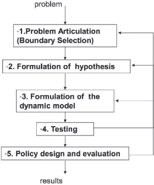
(7) 2.. Method - System dynamics. 2.1. Introduction. System dynamics is a computer-aided, mathematical approach to understanding dynamic behaviors of complex systems, ranging from social, economic or ecological systems to other multi-disciplinary ones (System Dynamics Society, 2015). The approach begins with problem articulation (boundary selection) and hypothesis formulation, based on which the development of the model is oriented. It, then, proceeds through mapping and modeling stages, building and testing the confidence in the model and finally its policy implications are yielded through simulation results (Sterman, 2000; System Dynamics Society, 2015).. The method was originally built during the mid-1950s by Professor Jay Forrester of the Massachusetts Institute of Technology as he was studying the counterintuitive behavior of social systems. Before that time, social issues were estimated mostly by contemplation, discussion, argument, and guesswork. Professor Forrester considered social systems as multiloop nonlinear feedback systems and that social issues were so complex that it needed to be studied with “an approach that combines the strength of the human mind and the strength of today's computers”, so called System dynamics. He believed this combination would “lead to a better understanding of our social systems and thereby to more effective policies for guiding the future” (Forrester, 1971).. In fact, when complex situations are encountered, intuition is not reliable as mental models usually take into account one-way cause-effect relationships. Therefore, the structural feedback existing in most of these systems are accidentally neglected. With system dynamics approach, a computer model is built so as to portray the system. In that model, it is compulsory that each relationship is considered separately and sequentially. Each part of the problem, as a consequence, is thoroughly examined, which in the end leads to a greater understanding through several perspectives. In addition, because mathematical models are programed with explicit language, ambiguity is completely eliminated. The hypotheses upon which the model is constructed and the relationships between constituent elements are comprehensively clarified and are subject to discussion and revision. As a result, a model’s projections can be studied precisely and objectively (Martín, 2006).. 4.

(8) 2.2. The modelling process. Even though there are numerous ways of constructing a system-dynamics model, the whole procedure of each approach is, roughly speaking, similar to one another. The modelling process depicted by John Sterman in Business dynamics: Systems thinking and modeling for a complex world in 2000 was chosen to follow in the doing of this thesis. Steps of the process are illustrated in Figure 1.. Firstly, the problem must be identified with logical reasoning. What are the key variables and concepts that must be taken into consideration? The time boundary must also be determined. How far back in the past shall the investigation start and how far shall it end? In addition, reference modes must be constructed for later comparison with simulation result. The historical behaviors of the key variables and concepts in the model must be considered, along with briefly how these components are expected to behave in the future after simulation.. Secondly, dynamic hypothesis must be formulated. What are current theories of behaviors of the key variables and the model in general? Within the model boundary, it is crucial to formulate a dynamic hypothesis that explains the dynamics of the model or, in other words, endogenous consequences of the feedback structure. Based on the relations between key components of the model, which are shown in those initial hypotheses and reference modes, maps of causal structure are to be built in the form of model boundary diagrams, causal loop diagrams or stock and flow maps.. 5.

(9) Figure 1: The modelling process (Sterman, 2000). Next, the model is built as its structure is concretely defined. While the initial conditions and historical values are set, parameters are estimated and variables are linked to each other with equations that illustrate their behavioral relationships. Some primary, basic tests are carried out in this step so as to inspect the consistency with the initial purpose and boundary of the model.. The following is to test how the model functions. The problem behavior that the model reproduce must be compared to reference modes in order to see if it suits the purpose. How realistic of the model under different practical conditions and assumptions must also be examined. Furthermore, it is vital to examine the sensitivity of the model. Changes in the behaviors of the model given uncertainty or alteration in parameters, initial conditions, model boundary, or aggregation must be taken into account. Providing the model fails to portray the issue practically, go back the first three steps to make adjustments.. Finally, from the simulation results of different scenarios, policies can be devised. How realistic and impactful one decision is in comparison with the others can be reviewed given the model’s behaviors. If the results yielded and policies suggested from the model suit the initial purpose is eventually evaluated here. Modifications in the previous steps can still be made until the desired information are collected.. 6.

(10) 2.3.. Several basic concepts in System dynamics. 2.3.1. Casual diagram. Once the key elements and the hypothetical relationships between the variables are known, a graphical representation called the casual diagram can be produced. It represents the key elements of the system and the relationships between them (Martín, 2006). The diagram “consists of variables connected by arrows denoting the causal influences among the variables” (Sterman, 2000). It is crucial to plot such figures that guide the modeler to construct the final complex model because the diagram can serve as the basic structure of the system.. In the diagram, the variables are linked with each other by arrows, known as casual links. Each arrow is assigned with a polarity, either positive (+) or negative (-), which indicates the kind of influence that one variable exerts over the other. A positive link means a change in the influencing variable will result in a change of the same direction in the target variable while a negative means the effect will be the opposite (Martín, 2006; Sterman, 2000).. Figure 2: Positive and negative casual links. As in Figure 2, when an increase in A leads to a rise in B, or a drop in A causes a fall in B, this is a positive relationship and when the effect happens the other way around, it is a negative link.. 2.3.2. Feedback loops. A feedback loop is a closed chain of relationships. As same as the casual links representing cause-effect relationships between variables, feedback loops are assigned with polarity too. In fact, the number of positive (or negative) links determines if a loop is positive (reinforcing) or negative (stabilizing). Loops are defined as positive if the number of negative relationships is even. Otherwise, they are negative (Martín, 2006).. 7.

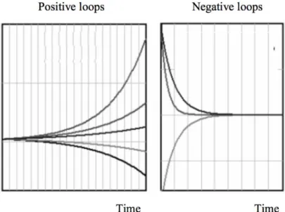
(11) Figure 3: Example of a stabilizing loop and a reinforcing one. For example, when an increase in population leads to an increase in birth, a rise in birth also causes a rise in population, making this a reinforcing loop (in the right of Figure 3). As for the relationship between population and food availability (in the left of Figure 3), more population means more food consumption, making the availability decrease while more food gives way for population growth. The feedback loop in this case is stabilizing (or balancing).. While negative loops tend to stabilize the model, positive loops tend to destabilize it (Martín, 2006). From the example above, it can be seen that the both of the two variables of the reinforcing loop have the trend to change in the same direction and the change in one variable shall strengthen the same change in the other. As for the negative loop, the model tends to move to a stable state. Figure 4 reflects how the models behave upon the characteristic of the loops they have.. Figure 4: Graphs representing the behaviors of models having two kinds of loops (Martín, 2006). 8.

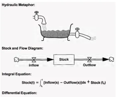
(12) 2.3.3. Stocks and flows. Causal loop (feedback) diagrams are extremely useful in many situations as they manage to represent interdependencies and feedback processes. They can capture the basic structure of the whole model at the very beginning of a modeling project. They are also used to communicate the results of a completed modeling effort. However, their inability to capture the stock and flow structure of systems makes it impossible to construct the model on a computer as well as inputting equations into the variables. The flow diagram (also known as the Forrester Diagram) that consists of stocks and flows is, therefore, used as a translation of the causal diagram. These are the two central concepts of dynamic systems theory (Martín, 2006; Sterman, 2000). “Stocks are accumulations. They characterize the state of the system and generate the information upon which decisions and actions are based. Stocks give systems inertia and provide them with memory” (Sterman, 2000). They are represented by rectangles in the diagram. As for flow variables, they constitute the ‘stock variation’. The integral of the difference between its inflow and its outflow is the stock. Flow is represented by a valve sign (Martín, 2006; Sterman, 2000). The notations for stocks and flows and their mathematical relationships are shown in Figure 5. Another kind of notation that is included in Forrester diagrams are clouds. They stand for the sources and sinks of the flows, both are not inside the boundary of the system (Sterman, 2000).. Figure 5: Hydraulic metaphor and the Forrester diagram (Sterman, 2000). 9.

(13) The hydraulic metaphor shown in Figure 5 a typical example illustrating the relations between inflow, outflow and stock. The volume of water contained in the bathtub is the stock in this diagram. The water going in from the tap on the left of Figure 5 is the inflow while the outflow goes through the second tap. The valve signs mean both the inflow and the outflow act as the stock regulators. Mathematically, the stock is an integral of the net change. The equation is show in Figure 5.. As for the remaining elements, they are categorized as auxiliary variables. These are used to the other variables that have algebraic relations with stocks and flows. Even though there are no strict process or rules in which how a variable is classified, when a casual diagram is transformed into the Forrester diagrams, the elements left after stocks and flows are identified are all auxiliary variables (Martín, 2006).. 10.

(14) 3.. Description of the model. 3.1.. Overview of the model. The model is built using software Vensim DSS 7.2 and historical and hypothetical data are stored in an Excel file. The name of the model is also the name of this thesis: Modelling of the dynamics of agroecological soil management and diet in the MEDEAS model framework. The timeline in which the study is conducted is from 1995 to 2050, with the projections starting from 2015. The hypothesis based on which the model is built is: “Switching to plant-based diets would not only guarantee to successfully feed the global populace, but also lead to a decrease in the need for agricultural land and help to mitigate the peak-oil effect on crop production”. This complies with the objective stated in the Introduction. The model is developed to demonstrate the relations of agricultural land use with dietary changes and with peak oil effect. The simulation result shall tell if the hypothesis is right.. With a clear goal, we construct the model with three main variables at its core, namely: •. Crop production yield: Historical values from 1995 to 2014 are collected from FAOSTAT. From the data, the historical trend of yield is estimated and BAU (business as usual) projections are extrapolated. As peak-oil has a direct effect on crop production yield, this impact is quantified and included in the projection of yield once the peak-oil effect is “activated”.. •. Crop demand - based on different diets: As population grows, food demand consequently increases. This leads to an increase in crop demand no matter how the diets are. If more meat is consumed, more fodder crops are grown to feed animals. If less meat is consumed, more crops eaten by human are needed to replace the nutrients that meat is supposed to provide. Therefore, each dietary choice has a unique impact on crop demand and these differences are comparable. Moreover, crop production relates directly with yield, which is influenced by peak oil effect. Choosing crop demand to represent food demand, instead of including meat consumption, suits the objective of the study.. •. Demand for agricultural land – based on different diets: The simulation result of this. 11.

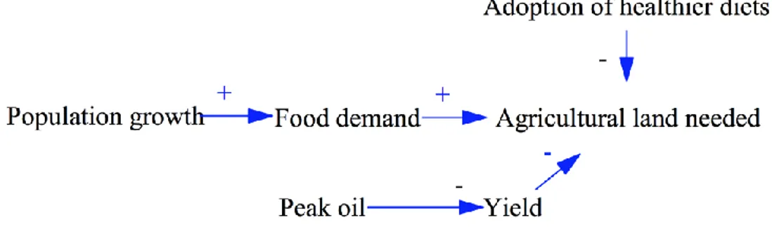
(15) variable demonstrates both the influence of peak oil effect and the impacts of changes in dietary patterns on agricultural land. It is calculated by dividing the crop demand with the crop production yield. Comparison between results of different diet scenarios shall yield if changing diets can be the solution to the problem of both restricted land use and peak oil effect.. 3.1.1. Casual diagram. The dynamics between variables are illustrated in the casual diagram (Figure 6). Population growth leads to an increase in food demand and in turn an increase in the demand of agricultural land as well. However, if healthier, more plant-based diets are adopted, the amount of area needed for agriculture decreases. Even though that means more types of crops are grown to compensate the nutrients and energy intake that meat normally offers, it has been proven that agricultural land is going to drop as a great amount of pastures and land for growing fodder crops are no longer needed (Fazeni & Steinmüller, 2011; S R Nadathur et al., 2017; Stehfest et al., 2009). The casual effect of peak oil is another crucial factor in the diagram. With the cultivation method still relying heavily on fossil fuels, production yield is expected to decrease, which shall increase the need for more agricultural land so as to make end meets due to the loss of productivity. Therefore, from the diagram alone, it is safe to claim that peak oil phenomenon can heat up the competition for surface area.. Figure 6: Casual diagram of the model. 3.1.2. Assumptions and model boundaries •. Without the effect of peak oil, crop production yield is extrapolated linearly based on the historical trend as advancements in science and technology are assumed to improve. 12.

(16) the cultivation techniques. •. While the historical values of crop production yield and cropland are collected from FAOSTAT, data of diets changes and values of pastures needed are derived from Stehfest et al., 2009, a study that investigates the impacts of changes in dietary pattern on the environment, including allocation of agricultural landuse. How datas are processed is to be described in following sections.. •. Production of coffee, vanilla, fiber crops and several other crops is not studied. Since the study is focus on impacts of dietary changes, the model only concerns with crops that are fed to human and animals. In addition, although in the model there are historical data about the production of seven crops, production of only four crops namely cereals, oil-crops, roots and tubers and pulses are investigated in the context of peak oil and dietary changes. Much as we would like to include them, there are no data about vegetables, tree-nuts and fruits in Stehfest et al., 2009, the study based on which we build the diet scenarios.. •. Since there is a lack of standardization in the estimation of oil extraction (CapellánPérez et al., 2014), it is not easy to quantified exactly how oil reserves and production are projected to decline. Due to the limit of research time, detail estimation of peak oil phenomenon as well as how it may affect the crop production is not included in the model. However, as oil production is proven to have been actually decreasing by numerous studies, it is quite logical to claim that the peak-oil effect shall affect the current agriculture which has been heavily dependent on fossil fuels. In this model, it is assumed that crop production yield would decrease following a logistic model with 1% of decrease rate from 2025 thanks to peak oil phenomenon.. •. It is not until 2026 that peak oil effect is assumed to take place in this study. Although some studies suggested that global oil extraction has already reached its peak (Mediavilla et al., 2013), we think that it would take quite some time for the phenomenon to start having practical impacts.. •. It is assumed that the shift to healthier diets would start from 2020 and finish in 2050.. 13.

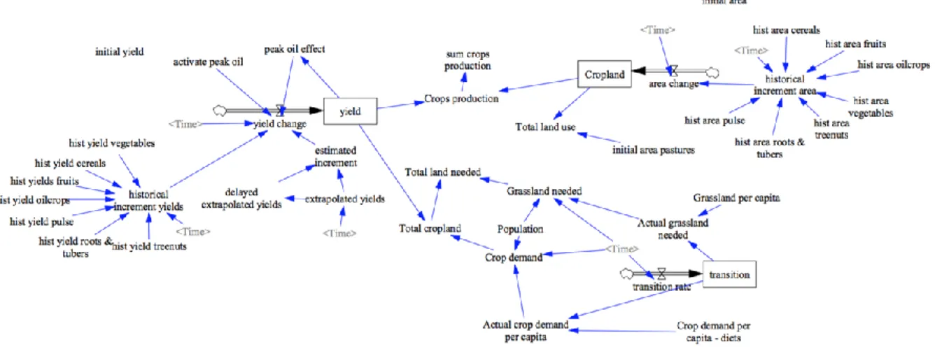
(17) Diet selection is quite complicated due to a wide variety of factors, ranging from the unique preference of each person to the transition in agricultural sector, adapting to such dietary changes. Therefore, if a change in global diet finally occurs, it is hard to expect the shift to happen quickly. •. From 2015, grassland and cropland are assumed to remain constant due to such immense pressures on agricultural land use from the productions of renewable energy, urbanization, etc.. •. Differences between farming methods are not taken into consideration in the model. Regardless of whether it is conventional and organic farming, the yield depicted in the model is calculated all the same.. •. Socio-economic factors are also neglected in the model. In practice, affluence, cultural impacts and lifestyle has major influences on food choice (Carolan, 2016; S R Nadathur et al., 2017). Food price is another factors that may have impacts on agricultural production and diet composition (Neacsu, McBey, & Johnstone, 2016). However, with the aim to investigate how dietary changes affect agricultural land-use, these factors are left out so as to simplify the model.. 3.2.. Forrester stock-flow diagram and description of variables. The model contains 42 variables, including 3 pairs of stock-flow variables. Even though the three main variables are crop production yield, crop demand and demand for agricultural land (yield, crop demand and total land needed in the diagram), the descriptions of the variables and explanations of equations are divided into three parts, corresponding to 3 pairs of stockflow variables in the model.. 14.

(18) Figure 7: Forrester stock-flow diagram of the model. 3.2.1. Historical cropland. Historical values from 1995 to 2014 of cropland area are collected from FAOSTAT. The data are gathered and put into a Microsoft Excel file. The numbers are extracted again by the Look-up equations of variables on Vensim.. In the model there are data about area allocated to grow seven main crops that are fed to human and animals (cereals, fruits, oilcrops, treenuts, roots and tubers and pulses). The ideas of having these values are: •. To witness the historical trend of cropland as a whole and for each type of crop.. •. To have areas of land that are used to grow each type of crop in 2014. This allocation of cropland is assumed, in the model, to remain the same in the future. Having this information separated for each crop is necessary as we would need it to calculate the crop production quantity by each crop in order to see if enough crop could be produced given the effect of peak oil and that agricultural land could not be expanded.. 15.

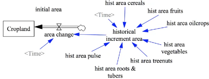
(19) Figure 8: Stock-flow diagram of historical cropland. Figure 8 shows how the historical values of cropland are adopted into the model. Cropland and area increase are the stock and flow variables. The unit of Cropland is ha (hectares) while it of area increase is ha/year. Cropland, area change, historical increment area and initial area are set as vectors so that they can represent seven values corresponding with seven types of crop. The area of land for growing cereals, for example is calculated as follows: initial area[cereals] 2 = 6.85428e+08 Unit: ha. The variable is the value of cereals’ area in 1994.. hist area cereals = GET XLS LOOKUPS('Historic data.xlsx', 'Area', '1', 'C3') Unit: ha/year. The variable represents the annual increment in area of cereal. It retrieves the data from the Excel file.. historical increment = IF THEN ELSE( Time<2014, hist area area[cereals] cereals(INTEGER(Time)),0) Unit: ha/year. The variable equals to the annual increment in area of cereal until 2014. After that, it is set to be 0 as cropland is assumed to remain constant. area change[cereals] = IF THEN ELSE(Time<2014, historical increment area[crops],0) Unit: ha/year. The same explanation for the previous equation is applied for this case. This step is, in fact, to transform data from auxiliary variable into flow variable.. 2. Subscripts are enclosed in square brackets [ ] directly following the variable name. In this case it is Cereals.. 16.

(20) Cropland[cereals] = Initial area[cereals] + area change[cereals] Unit: ha. The stock is the sum of initial value and area increment accumulated each year. In short, so as to calculate the cereals’ area by year, the stock is added hist area cereals (which stands for historical increment of cereals’ area) in each year. This is repeated until 2014, when no historical data are provided and the cropland is assumed to remain constant from that point on. Because the amount of area used to grow each crop is calculated in the exact same way, only the calculation of cereals’ area is illustrated. The historical trend of cropland by each crop is illustrated in Figure 93.. 3. There are two graphs shown because the areas for cereals and oilcrops are much greater than the others. Putting them all in the same graph would make it hard to see historical trend of each crop.. 17.

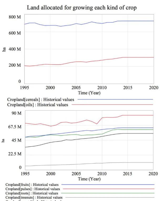
(21) Figure 9: Historical values of cropland, by each crop. From Figure 9, it can be easily pointed out that cropland was expanded from 1995 to 2014. Even though some fluctuations were recorded, increasing is the overall trend. Area used for producing cereals seems to be the only one that remains quite stable. However, in fact, it did increase, form 685.4 Mha (million hectares) in 1995 to 722.9 Mha in 2014. We believe that this trend is reasonable as the population grows, more land should be used for crop production. Nevertheless, it is illogical to have this trend increase indefinitely, given the fact that the competition for land has been heated recently. This is the reason why we assume that from. 18.

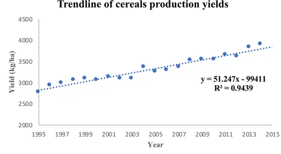
(22) 2015, agricultural land including cropland remained constant, which is also shown in the graphs.. Now that area used for crop production is calculated, land available for agriculture can be calculated as well. It will be used to compare with the total areas of land needed by each diet scenario. The variable is the sum of cropland and grassland area (Figure 10). Available grassland is a constant value, showing the area of land used for livestock production in 2014.. Figure 10: Calculation of land available for agricultural production. 3.2.2. Historical values and extrapolation of yield. Historical values from 1995 to 2014 of yield are collected from FAOSTAT. As how the data are inputted as same as the historical values of cropland, it is not described again. In this section, how the linear extrapolation of yield and peak-oil effect are executed in the model is described. Figure 11 shows how all of these factors are linked together.. Figure 11: Stock-flow diagram of yield including the extrapolation and peak-oil effect. As the procedure of extrapolating production yield is the same for all types of crop, yield of cereals is chosen as an example to explain how it is done. Based on the historical values. 19.

(23) provided by FAOSTAT, the linear trend-line and extrapolation equation can be formed using Microsoft Excel (Figure 12). This equation is then adopted in the model, under the variables extrapolated yields.. Trendline of cereals production yields 4500. Yield (kg/ha). 4000 3500. y = 51.247x - 99411 R² = 0.9439. 3000 2500 2000 1995. 1997. 1999. 2001. 2003. 2005. 2007. 2009. 2011. 2013. 2015. Year. Figure 12: Linear trend-line and extrapolation equation of cereals’ yield. The unit of Yield is kg/ha (kilograms/hectare) while it of the others is kg/ha/year. Yield, yield change, estimated increment, extrapolated yields and delayed extrapolated yields are set as vectors so that they can represent seven values corresponding with seven types of crop. Calculation of peak oil effects on yield is also included in this part of the model. As its effects on each crop production yield is different, peak oil effect variable is also a vector, with subscript is the type of crops. The extrapolation of cereals crop production is calculated as follows:. extrapolated yields = IF THEN ELSE( Time>=2013,Time*51.247-99411,0) [cereals] The extrapolation using the linear equation starts in 2013.. delayed extrapolated = extrapolated yields[cereals], 1, 0 yields [cereals] The extrapolated value is delayed for one year.. estimated increment = extrapolated yields[cereals]-delayed extrapolated yields[cereals] [cereals] The increment equals the extrapolated value minus the delayed value. For example, the increment in 2015 equals the extrapolated value of 2015 minus the 2014 one.. 20.

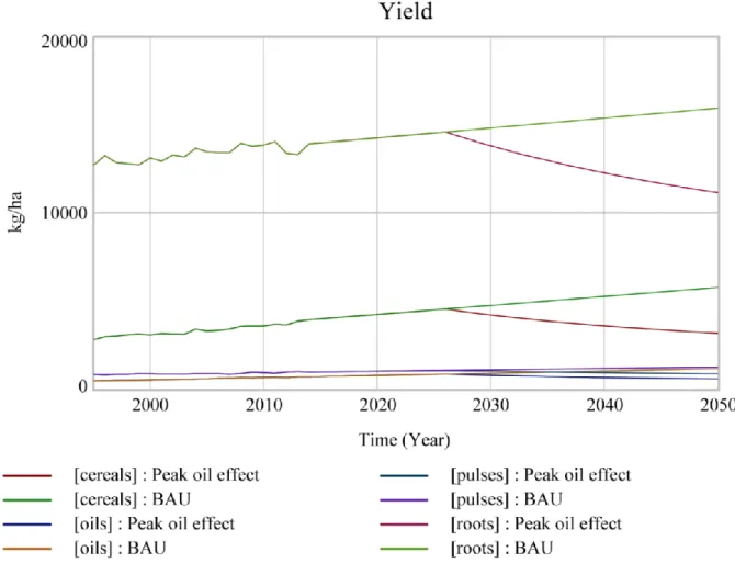
(24) peak oil effect = yield[cereals]*0.01*(1-(yield[cereals]/1979)) [cereals] The equation takes after the logistic model with goal-seeking degrowth.. activate peak oil Set to be either 1 or 0. 1 means peak oil effect is represented in the model. Otherwise, the yields follow theirs BAU extrapolation.. yield change[cereals] = IF THEN ELSE(Time<2014, historical increment yields[cereals],IF THEN ELSE(Time>2025:AND:activate peak oil=1, peak oil effect[cereals] , estimated increment[cereals])) From 1995 to 2014, yield change equals the historical increment. From 2015, it is the extrapolated increment. If the peak oil effect is “activated”, from 2026, yield change is peak oil effect. Otherwise, the variable remains to be the extrapolated increment.. yield[cereals] = initial yield[cereals] + yield change[cereals]. Since the scenarios of dietary changes (explained in section 3.3) are concerned with four crops namely cereals, oilcrops, roots and tubers and pulses, the peak oil effect is only applied for the production yield of these four crops.. Even though how the yield is calculated is quite complicated, doing it this way, instead of extrapolating in and get all the results from the Excel file, helps to show distinctively how historical values and extrapolation are calculated in the Vensim model.. Behaviors of projected yields are illustrated in the Figure 13. There is no doubt that peak oil effect is going to reverse the increasing trend of production yield if the global agriculture still relies heavily on fossil fuels.. 21.

(25) Figure 13: Crop production yield - with and without peak oil effect. 3.2.3. Transition of global diets and its impact. The transition of diets leads to changes in crop demand and livestock production, which ultimately affect cropland and grassland needed. As it takes time for a global change in dietary patterns to take place, the effects are projected to occur gradually. Therefore, this whole dynamic shift is driven by stock-flow variables in transition and transition rate (Figure 15).. 22.

(26) Figure 14: Impact of dietary changes on demand for agricultural land. Following are the equations demonstrating how the transition works: transition rate = IF THEN ELSE( Time<2020 , 0 , (1-0)/(2050-2020) ) The transition is assumed to last from 2020 to 2050. The rate can be understood as a percentage of the new diet is being followed by the global populace every year or a portion of the population is adopting the new diet. Or this can also be understood as the transition in agricultural production to meet the new demand.. transition = transition rate The value is the accumulation of increment each year.. The scenarios are built based on the work of Stehfest et al., 2009. For each diet, they provided the values of production quantity and agricultural land (Figure 16). These are the final results of the transition process, all in 2050. However, in this study, using system dynamic method we would like to see how the transition takes place and its effects along the whole process. Therefore we calculate the production quantity and grassland needed per capita in 2050 and for each year, to have the crop production and grassland needed, we multiply these two parameters with the population, which is deried from (United Nations Department of Economic and Social Affairs Population Division, 2017) and the WoLim model. Transition is added in the equations so as to see the beahaviors of these varibales during the shift. The equations used in this sections are described, as follows: Crop demand per = GET XLS CONSTANTS('Historic data.xlsx', 'Food capita' , 'B2' ) capita – diets Unit: kg/person. The value, for each diet and for each crop is already. 23.

(27) [diet,crop] calculated in the Excel file. The equation is used to extract these numbers. In this case, the value of cereals produced for the first diet is looked up.. Actual crop demand = "Crop demand per capita - diets"[present,crop]*(1per capita [diet,crop] transition)+"Crop demand per capita - diets"[diet,crop]*transition Unit: kg/person. Only a ratio of population adopts the new diet or only a part of the diet is being followed. The rest remains the same as present diet.. Crop demand = Population(Time)*Actual crop demand per capita[Diet,crop] [diet,crop] Unit: kg. Crop demand for each diet, each crop is calculated.. Total cropland[diet] = Crop demand[Diet,cereals]/Yield[cereals]+Crop demand[Diet,oils]/Yield[oils]+Crop demand[Diet,roots]/Yield[roots]+Crop demand[Diet,pulses]/Yield[pulses] Unit: ha. Total cropland needed for each diet is calculated.. Grassland per capita = GET XLS CONSTANTS('Historic data.xlsx', 'Grassland' , 'B1' ) [diet] Unit: ha/person. The grassland need per each person is already calculated in the Excel file.. Grassland needed = Population(Time)*Actual grassland needed[Diet] [diet] Unit: ha. Actual grassland needed[Diet] is calculated the same as Actual crop demand per capita [diet,crop].. Total land needed = Total cropland[Diet]+Grassland needed[Diet] [diet] Unit: ha.. 24.

(28) 3.3.. Scenarios of diets. Dietary patterns are adopted from Stehfest et al., 2009. The study provies information about crop production and grassland needed for each scenario. However, as mentioned in section 3.2.3, these data are calculated for the year 2050. As for our study, we seek to record the beahaviors of these parameters throughout the progress of transition, not just being focus on the final outcome in 2050. Therefore, these numbers are divided with the global population projected in the study. With the crop demand and grassland needed per capita, we can calculate the these two figures every year using estimation of the population. The results are to be compared with projected crop production and land availability to see how changing diets are impactful and if switching to such dietary patters are feasible.. Figure 15: Crop production and land use by each diet (Stehfest et al., 2009) Table 1: Adoption of dietary scenarios of Stehfest et al., 2009 into this model. Variant. Scenarios in this study. Description. (Stehfest et al., 2009) (Stehfest et al., 2009) Reference. Agricultural production for 2000–2030 More meat (MoreM) (Bruinsma 2003) and 2030–2050 (FAO 2006).. No Meat (NoM). As reference, but with complete substitution No Meat (NoM) of proteins from ruminant meat (cattle, buffaloes, sheep and goats), white meat (pork, poultry) by plant proteins by plantproteins.. No Animal. As NoM, with additional substitution of milk No Animal Products. 25.

(29) Products (NoAP). and eggs by plant proteins. (NoAP). Healthy Diet. “Healthy Eating” recommendations from the Healthy Diet. (HDiet). Harvard Medical School (Willett 2001) (Healthy) implemented globally for meat and eggs. Only four crops, namely cereals, oilcrops, roots and tubers and pulses, are considered in Stehfest et al., 2009. The reference scenario of their study is interpreted as More meat (MoreM) because with their projection, the increasing trend of meat production and consumption is maintained. Many countries, including China, is expected to adopt more animal-based diet. In this study, moreM is the baseline scenario for future projection. As for the present scenario in our study (applied from 1995 to 2014), the diet is assumed to be as same as the diet composition in 2000 in Stehfest et al., 2009. Even though it is not so convincing to suppose the diet in 2000 would remain the same for a decade later, due to the time limit, we still choose to do it this way. Regarding the healthy diet, this means that more plant-based products are included in the diet while meat is still consumed at a reasonable level, which is certainly lower than the meat consumption in Western diet (Willett 2001).. Table 2: Annual crop demand per capita (kg/person) for each diet. Present. MoreM. NoM. NoAP. Healthy. Cereals. 295.328. 312.872. 244.561. 216.313. 273.689. Oilcrops. 26.628. 44.131. 33.524. 29.281. 44.186. Roots&Tubers. 21.786. 27.006. 22.533. 20.444. 22.423. Pulses. 30.259. 50.718. 81.337. 103.540. 58.035. Table 2 shows the crop demand per capita based on each diet. Stehfest et al., 2009 assumed that meat, egg and milk proteins (including milk and all dairy products such as butter and cheese) are substituted by proteins from pulses and soybeans in all variants. Therefore, as it can be seen from the table, the less meat or animals’ products are consumed, the more pulses are needed to provide enough proteins. As for grassland, the area need for livestock production per person is represented in Table 3. Such difference between the values of moreM and present scenario can be easily spotted. While the value of present is actually calculated for the year 2000, that of moreM is estimated for 2050. This is due to the fact that moreM scenario involves more animals’ products and according to Stehfest et al., 2009, more meat, eggs and milk is produced in mixed and landless system than in pastoral system.. 26.

(30) Table 3: Annual grassland per capita, by each diet (ha/person). Diet Grassland per capita (ha/person). Present 0.546. 27. MoreM 0.345. NoM 0.0534. NoAP. Healthy 0. 0.2.

(31) 4.. Result and discussions. 4.1.. Simulation result without peak oil effect. Figure 16: Land demand for food production by each diet - BAU. As the yield is projected to increase gradually without peak oil effect, land demand for food production is dependent heavily on the population growth and dietary changes. Overall, the simulation result turns out to be quite reasonable since moreM diet, involving the highest meat consumption, would require the largest areas. From Figure 17, it can be stated that changes in dietary patterns have a major impact on agricultural production. Switching to more plant-based diet can cut down a significant proportion of agricultural land.. Before the dietary changes take place, present diet makes total land needed increase as population growth outruns the growth in crop production yield. As the animals’ products are consumed a lot in this dietary composition while the annual grassland per capita is quite high in comparison with other future diets, this behavior is understandable. To be more specific, the present diet needs more areas than land availability in the period from 2018 to 2020 (recorded respectively at 5.202; 5.243 and 5.278 billion hectares versus 5.184 billion hectares available), right before the transition begins to happen. Had it not been for the changes in diets, the land. 28.

(32) demand would go way beyond the available areas. This is due to such a great amount of grassland needed per capita in present scenario.. As for the transition, dietary changes are proven to be so effective. In comparison with moreM scenario, which also is the diet that the global populace is expected to adopt, healthy scenario needs much less land. The effect of noM and noAP is even more impressive. The detail decrease in land demand by each diet is represented in Table 4. In 2050, when the transition is finished, with moreM scenario, thanks to the growth of production yield, 13% of available agricultural land would no longer be need. However, this percentage of healthy diet is 39%, tripe moreM scenario.. Table 4: Total land needed by each diet in 2050 - BAU. Total land need (ha). Redundant land (ha). % of available land. moreM. 4.508 billion. 0.676 billion. 13%. noM. 1.811 billion. 3.373 billion. 65%. noAP. 1.399 billion. 3.785 billion. 73%. healthy. 3.141 billion. 2.043 billion. 39%. In short, with respect to land demand, adoption of healthier diet (more plant-based) will take off significantly some of the immense pressures on the need for agricultural land expansion.. 4.2.. Simulation result with peak oil effect. With the effect of peak oil, the yield starts decreasing from 2026. In this case, pressures on land demand for food production do not only come from the population growth but also from the decreasing crop production yield. Overall, in comparison with BAU scenario, the land demand in all four dietary scenarios are significantly higher. This is explainable as the land has to be expanded so as to make up for the drop in yield. It can be seen from Figure 18 that switching to more plant-based diet can overcome the problem of increasing agricultural land caused by peak oil effect.. 29.

(33) Figure 17: Land demand for food production by each diet – Peak oil effect. Indeed, dietary changes are proven to be so impactful. The simulation result yielded in this case is similar to the BAU scenario. In comparison with moreM scenario, which can be considered as the baseline, healthy scenario needs much less land. Despite a substantial drop in yield, the agricultural sector would still be able to provide the global populace a healthy diet without using up the available land. Meanwhile if the increasing trend of meat consumption is maintained, the land demand for moreM diet is projected to be greater than the land availability. The adoption of noM and noAP, without a doubt, would save much more land. The final result in land demand by each diet is represented in Table 5. In 2050, when the transition is finished, with moreM scenario, due to a decrease in production yield, 2% more of available land is needed in order to meet the land demand. (negative in the table means lack of land). As for healthy diet 24% of available land, equaling more than 1 billion hectares would no longer be need and ready for other purposes.. 30.

(34) Table 5: Total land needed by each diet in 2050 - Peak oil effect Total land need (ha). Redundant land (ha). % of available land. moreM. 5.305 billion. - 0.121 billion. - 2.3%. noM. 2.582 billion. 2.602 billion. 50%. noAP. 2.194 billion. 2.990 billion. 58%. healthy. 3.925 billion. 1.259 billion. 24%. In short, with respect to land demand, adoption of healthier diet (more plant-based) is the solution to overcome the effect of peak oil on agricultural land use.. 4.3.. Limitations and implications of the model. 4.3.1. Limitations of the model •. We based our data on the paper Stehfest et al., 2009 and they assumed that healthy and. vegetarian and other diets are based on removing pastures, this approach is not the only possible or even reasonable and therefore our results are heavily dependent on it. •. To cope with peak oil, there are other ways to improve productivity. Organic is not. studied so far. Much as farming method, such as organic and conventional farming, has a crucial impact on energy use and land occupation (Bos, De Haan, Sukkel, & Schils, 2014; Treu et al., 2017), due to the limit of time and lack of data, the dynamic is not depicted in this model. In fact, while organic farming has less environmental impacts and consumes less fossil fuels, the fact that it requires, in return, great areas of land makes it hard for farmers to apply the method itself. This is such an interesting facet that the model unfortunately cannot include.. 4.3.2. Implications of the result. As the simulation results are presented above, the proposed changes in dietary patterns have a major impact on the management of agricultural land use. Adoption of healthier diet, with more plant-based products instead of animal-based, would release the pressures of land expansion, even if peak oil effect finally occurs. This can potentially be the ultimate key. 31.

(35) solution to overcome the decrease in yield and population growth. Indeed, this may be a better solution than organic farming (use less oil but need far more land) as it fixes the problem at the consumers’ side.. 32.

(36) CONCLUSION. The study managed to investigate the historical trend of yields, conduct the extrapolation of yields and study food production for main crops. A system dynamics model is designed and built so as to study the production of the main crops in the context of peak oil effect, growing yields and different diets. The simulation results show that if present trends of more meat consumption are continued, this can be problematic for the agricultural sector providing the amount of agricultural land cannot grow, which is a realistic assumption because of growing urbanization, competition for surface land with biofuels, solar plant, etc. A shift in dietary patterns to healthier, more plant-based diets can potentially can potentially overcome these issues. In case peak oil finally occurs, maintaining the heavily-animal-based diet may even be impossible. The research shall be carried on with more deep studies of diets and land occupation. Even though this is just the first step, it still serves as preliminary valuable evidence of the important effects of diet on agricultural production.. 33.

(37) REFERENCES. Bos, J. F. F. P., De Haan, J., Sukkel, W., & Schils, R. L. M. (2014). Energy use and greenhouse gas emissions in organic and conventional farming systems in the Netherlands. NJAS - Wageningen Journal of Life Sciences, 68, 61–70. https://doi.org/10.1016/j.njas.2013.12.003 Bruinsma JE (2003) World agriculture: towards 2015/2030. An FAO perspective. Earthscan, London Capellán-Pérez, I., de Castro, C., & Arto, I. (2017). Assessing vulnerabilities and limits in the transition to renewable energies: Land requirements under 100% solar energy scenarios. Renewable and Sustainable Energy Reviews, 77(September 2016), 760–782. https://doi.org/10.1016/j.rser.2017.03.137 Capellán-Pérez, I., Mediavilla, M., de Castro, C., Carpintero, Ó., & Miguel, L. J. (2014). Fossil fuel depletion and socio-economic scenarios: An integrated approach. Energy, 77, 641–666. https://doi.org/10.1016/j.energy.2014.09.063 Carolan, M. (2016). Food Security and Policy. Sustainable Protein Sources. Elsevier Inc. https://doi.org/10.1016/B978-0-12-802778-3.00024-X De Castro, C., Mediavilla, M., Miguel, L. J., & Frechoso, F. (2013). Global solar electric potential: A review of their technical and sustainable limits. Renewable and Sustainable Energy Reviews, 28, 824–835. https://doi.org/10.1016/j.rser.2013.08.040 Diouf, J. (2009). DOCUMENTS FAO ’ s Director-General on How to Feed the World in 2050. World, 5, 837–839. https://doi.org/10.1111/j.1728-4457.2009.00312.x FAO (2006) World agriculture: towards 2030/2050. Prospects for food, nutrition, agriculture and major commodity groups, Food and Agriculture Organization of the United Nations, Global Perspective Studies Unit, Rome. 34.

(38) Fazeni, K., & Steinmüller, H. (2011). Impact of changes in diet on the availability of land , energy demand , and greenhouse gas emissions of agriculture, 1–14. Forrester, J. W. (1971). Counterintuitive behavior of social systems. Theory and Decision, 2(2), 109–140. https://doi.org/10.1007/bf00148991 Gomiero, T. (2016). Soil degradation, land scarcity and food security: Reviewing a complex challenge. Sustainability (Switzerland), 8(3), 1–41. https://doi.org/10.3390/su8030281 Koh, L. P., Miettinen, J., Liew, S. C., & Ghazoul, J. (2011). Remotely sensed evidence of tropical peatland conversion to oil palm. Proceedings of the National Academy of Sciences, 108(12), 5127–5132. https://doi.org/10.1073/pnas.1018776108 Martín, J. (2006). Theory and Practical Exercises of System Dynamics. System. Mediavilla, M., de Castro, C., Capellán, I., Javier Miguel, L., Arto, I., & Frechoso, F. (2013). The transition towards renewable energies: Physical limits and temporal conditions. Energy Policy, 52, 297–311. https://doi.org/10.1016/j.enpol.2012.09.033 Nadathur, S. R., Wanasundara, J. P. D., & Scanlin, L. (2017). Chapter 1 - Proteins in the Diet: Challenges in Feeding the Global Population. In S. R. Nadathur, J. P. D. Wanasundara, & L. B. T.-S. P. S. Scanlin (Eds.) (pp. 1–19). San Diego: Academic Press. https://doi.org/https://doi.org/10.1016/B978-0-12-802778-3.00001-9 Neacsu, M., McBey, D., & Johnstone, A. M. (2016). Meat Reduction and Plant-Based Food: Replacement of Meat: Nutritional, Health, and Social Aspects. Sustainable Protein Sources. Elsevier Inc. https://doi.org/10.1016/B978-0-12-802778-3.00022-6 Stehfest, E., Bouwman, L., Van Vuuren, D. P., Den Elzen, M. G. J., Eickhout, B., & Kabat, P. (2009). Climate benefits of changing diet. Climatic Change, 95(1–2), 83–102. https://doi.org/10.1007/s10584-008-9534-6 Sterman, J. D. (2000). Business dynamics: Systems thinking and modeling for a complex world. Management. https://doi.org/10.1057/palgrave.jors.2601336. 35.

(39) System Dynamics Society. (2015). What is System Dynamics « System Dynamics Society. System Dynamics. Retrieved from http://lm.systemdynamics.org/what-is-s/ Tomczak, J. (2013). Implications of Fossil Fuel Dependence for the Food System. Resilience. Retrieved from http://www.resilience.org/stories/2006-06-11/implications-fossil-fueldependence-food-system Treu, H., Nordborg, M., Cederberg, C., Heuer, T., Claupein, E., Hoffmann, H., & Berndes, G. (2017). Carbon footprints and land use of conventional and organic diets in Germany. Journal of Cleaner Production, 161, 127–142. https://doi.org/10.1016/j.jclepro.2017.05.041 UNCCD. (2017). Global Land Outlook. First Edition. Secretariat of the United Nations Convention to Combat Desertification. https://doi.org/ISBN: 978-92-95110-48-9 United Nations Department of Economic and Social Affairs Population Division. (2017). World Population Prospects The 2017 Revision Key Findings and Advance Tables. World Population Prospects The 2017, 1–46. https://doi.org/10.1017/CBO9781107415324.004 van Vliet, J., Eitelberg, D. A., & Verburg, P. H. (2017). A global analysis of land take in cropland areas and production displacement from urbanization. Global Environmental Change, 43, 107–115. https://doi.org/10.1016/j.gloenvcha.2017.02.001 Willett WC (2001) Eat, drink, and be healthy: the Harvard Medical School guide to healthy eating. Simon & Schuster, New York https://doi.org/10.1093/aje/154.12.1160-a. 36.

(40)