TítuloTumor growth analysis using cellular automata based on the cancer hallmarks

(1)

Departamento de Computaci´

on

Tumor growth analysis using cellular automata

based on the cancer hallmarks

PhD Thesis

Tese de doutoramento

´

Angel Monteagudo Insua

(2)

(3)

PHD THESIS

Tumor growth analysis using cellular

automata based on the cancer hallmarks

´

Angel Monteagudo Insua

PhD supervisor:

Dr. Jos´e Santos Reyes

Thesis committee:

Dr. Amparo Alonso Betanzos

Dr. Rafael Lahoz Beltr´

a

(4)

(5)

D. Jos´

e Santos Reyes

, Profesor Titular de Universidad en el ´

area

de Ciencias de la Computaci´

on e Inteligencia Artificial de la

Uni-versidade da Coru˜

na

CERTIFICA

Que la presente memoria titulada

Tumor growth analysis

us-ing cellular automata based on the cancer hallmarks

fue realizada

bajo su direcci´

on y constituye la Tesis que presenta

D. ´

Angel

Mon-teagudo Insua

para optar al grado de Doctor por la Universidade

da Coru˜

na.

A Coru˜

na, diciembre de 2015

(6)

(7)

“Modern biology encourages us to imagine the cell as a molecular machine. Cancer is that machine unable to quench its initial command (to grow) and thus transformed into an indestructible, self-propelled automaton.”

(8)

(9)

Acknowledgments

I would like to mention, in the first place, my supervisor Jos´e Santos Reyes for letting me have the opportunity to do this PhD thesis. Thanks for all the help, suggestions and supervision during these years.

I want to thank the staff at theOncology Center of Galiciafor the technical advice and discussions about all the aspects of the modeling performed in the thesis.

I especially thank the members of our Lab in the Computer Science De-partment, and specially those with which I have shared the Lab these years, Mart´ın, Edu, Javier, V´ıctor, Rodrigo, Dani, as well as the rest of the members for all the help and good moments.

This research has been supported by grants from the Government of Spain (Projects TIN2013-40981-R and TIN2011-27294).

(10)

(11)

Abstract

In this thesis we used computational models based on cellular automata and the abstract model of cancer hallmarks to analyze the emergent behavior of tumor growth at cellular level. Tumor growth is modeled with a cellular auto-maton which determines cell mitotic and apoptotic behaviors. These behaviors depend on the cancer hallmarks acquired in each cell as consequence of muta-tions. The presence of the cancer hallmarks defines cell states and cell mitotic behaviors. Additionally, these hallmarks are associated with a series of para-meters, and depending on their values and the activation of the hallmarks in each of the cells, the system can evolve to different dynamics.

With the simulation tool we performed an analysis of the first phases of cancer growth. Firstly, we studied the evolution of cancer cells and hallmarks in different representative situations regarding initial conditions and paramet-ers, analyzing the relative importance of the hallmarks for tumor progression; Secondly, we focused on the analysis of the effect of killing cancer cells, in-specting the time evolution of the multicellular system under such conditions and the possible behavioral transitions between the predominance of cancer and healthy cells.

(12)

(13)

List of Tables

2.1 Definition of the parameters associated with the hallmarks . . . 20

(16)

(17)

List of Figures

1.1 Schematic view of the initial hallmarks considered in [39][40].

Figure reprinted with permission from Elsevier. . . 8

1.2 The effect of angiogenesis in tumor growth. A: When a tumor is small, cancer cells obtains oxygen and nutrients from surround-ing blood vessels. B: As the tumor grows beyond the capacity of local blood vessels, soluble pro-angiogenic growth factors are released which promote the sprouting of new vessels (neovas-cularization) from local pre-existing blood vessels. C: The new vessels provide a blood supply for the tumor enabling tumors to grow beyond 2–3mm3 in size. . . 10

1.3 Terapeutic Agents. Figure from [40], reprinted with permission from Elsevier. . . 11

1.4 Phases of the cell cycle. Figure reprinted with permission by Siyavula Education and made available atwww.everythingscience. co.zaunder the terms of a CC-BY 3.0 license [60]. . . 13

1.5 The PI3K/Akt/mTOR signaling pathway [54]. This pathway is up-regulated in a significant proportion of ovarian cancers. Figure reprinted with permission from InTech. . . 15

1.6 In the Cancer Stem Cell (CSC) model these cells can divide sym-metrically or asymsym-metrically to produce Differentiated Cancer Cells (DCCs) with limited proliferative capability. . . 17

2.1 Diagram of the event model. The rectangles indicate an action, a rhomb indicates a check with an associated binary question, as explained in the text. This process is repeated to all the cells in the grid environment. Each cell is represented with a small circle. If the cell dies after a check it is represented with a crossed-circle. . . 25

2.2 Event model used in the simulation. Mitoses are scheduled between 5 and 10 time iterations in the future. When a mitosis event is processed, several tests are performed to determine if the cell dies, continues quiescent or can perform the division (explained in Figure 2.1 and Algorithm 2.1.1). . . 26

2.3 Self-Growth hallmark rule. . . 28

2.4 Ignore Growth Inhibit hallmark rule. . . 28

(18)

xviii List of Figures

2.6 Effective Immortality hallmark rule. . . 29 2.7 Genetic Instability hallmark rule. . . 30 2.8 Evolution through time iterations of the number of healthy cells

(continuous lines) and cancer cells (dashed lines) for two differ-ent hallmark mutation rates (1/m) and default parameters. It also appears in continuous red line the fit curve for cancer cells using a Gompertz function. . . 31

3.1 Left: Evolution through time iterations of the number of healthy cells (continuous line) and cancer cells (dashed line) with m= 10000 and parameter default values. Center: Time evolution of the number of cells with a hallmark acquired. All the graphs are an average of 5 independent runs. Right: Example of a 2D cross-section of a final configuration at the end of the temporal evolution (at t= 1000). Healthy cells are shown in bright gray whereas the other colors correspond to different combinations of hallmarks acquired. . . 37 3.2 Left: Evolution through time iterations of the number of healthy

cells (continuous line) and cancer cells (dashed line) with m= 1000 and parameter default values. Center: Time evolution of the number of cells with a hallmark acquired. All the graphs are an average of 5 independent runs. Right: Example of a 2D cross-section of a final configuration at the end of the temporal evolution (att= 1000). . . 37 3.3 Left: Evolution through time iterations of the number of healthy

cells (continuous line) and cancer cells (dashed line) with m= 100 and parameter default values. Center: Time evolution of the number of cells with a hallmark acquired. All the graphs are an average of 5 independent runs. Right: Example of a 2D cross-section of a final configuration at the end of the temporal evolution (att= 1000). . . 38 3.4 Left: Time evolution of the number of healthy cells

(continu-ous line) and cancer cells (dashed line) with a parameter set which facilitates cancer growth. Center: Time evolution of the number of cells with a hallmark acquired. All the graphs are an average of 5 independent runs. Right: 2D cross-section of a final configuration at the end of the temporal evolution (at

t= 5000). . . 39 3.5 Snapshots of the cellular system at different time steps using

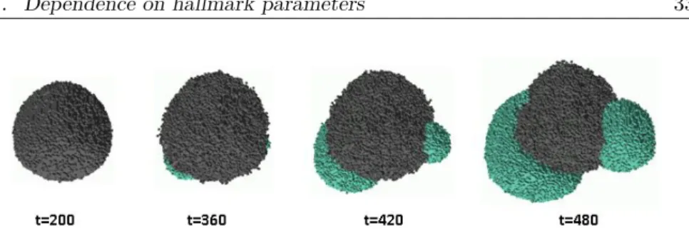
the parameter set of Figure 3.4 (Grid size=106_). _{. . . .} ₄₁

(19)

List of Figures xix 3.7 Number of final cancer cells when two parameters are changed,

while the rest of parameters are set at their default values, ex-cept m= 1000 (a and b). The z axis shows the final number of cancer cells after 1000 time iterations in the simulation. a) Change of parameterse(which controls EA) andg(IGI). b) the parameterse(EA) andi(GI) were changed. c) the parameters

m(hallmark mutation rate) andg (IGI) were changed. All the graphs are an average of 5 independent runs. . . 44 3.8 Left: Effect of elimination of an individual hallmark. Right:

Number of cancer cells when only one hallmark is considered. Simulations with parameter default values and m= 100, aver-aged with 5 independent runs. . . 46 3.9 Number of cancer cells when an individual hallmark is not

con-sidered (Left) and when only one hallmark is concon-sidered (Right). Simulations with parameter values of Figure 3.4, averaged with 5 independent runs. . . 47 3.10 Effect of killing cancer cells during tumor growth for different

killing probabilities and using four parameter sets. Thex-axis is interpreted as the probability of eliminating cancer cells in the mitotic average time during the simulation, whereas they-axis represents the final number of cancer cells. . . 51 3.11 Effect of killing cancer cells during tumor growth for different

killing probabilities and using four parameter sets. Thex-axis is interpreted as the probability of eliminating cancer cells in the mitotic average time during the simulation, whereas they-axis represents the final number of cancer cells. Only the most outer cells (distance of 3 or less to the boundary of the expanding tumor) are killed with the corresponding probability indicated in thex-axis. . . 54

4.1 Different models for cellular origin of cancer. Two models have been proposed to explain the cellular heterogeneity in cancer: the stochastic model and the hierarchical model. In the first one, every tumor cell can stochastically generate a tumor. In the second one, only the CSCs can generate tumors. Figure from [16], reprinted with permission from BioMed Central. . . . 59 4.2 In the Cancer Stem Cell (CSC) model these cells can divide

sym-metrically or asymsym-metrically to produce Differentiated Cancer Cells (DCCs) with limited proliferative capability. . . 62 4.3 Upper graph: Evolution through time iterations of the

num-ber of healthy cells (continuous line), non-stem or differentiated cancer cells (DCCs, dashed line) and Cancer Stem Cells (CSCs) (pointed line). CSCs are introduced at time iteration 100 (1% of the grid size) in the grid initially full of healthy cells. Standard hallmark parameters were used except g=5. At time iteration

(20)

xx List of Figures

4.4 Snapshots of 2D central sections of the multicellular system evolution corresponding to different time iterations in Figure 4.3 (Colors: Gray - healthy cells, Blue - DCCs, Red-enlarged size - CSCs). . . 66

4.5 Upper graph: Evolution through time iterations of the num-ber of healthy cells (continuous line), non-stem or differentiated cancer cells (DCCs, dashed line) and Cancer Stem Cells (CSCs) (pointed line). CSCs are introduced at time iteration 100 (1% of the grid size) in the grid initially full of healthy cells. Stand-ard hallmark parameters were used except m=1000. At t=6000 the 100% of DCCs is killed. Bottom graph: Evolution through time iterations of the different hallmarks in the cancer cells. . . 68

4.6 Snapshots of 2D central sections of the multicellular system evolution corresponding to different time iterations in Figure 4.5 (Colors: Gray - healthy cells, Blue - DCCs, Red-enlarged size - CSCs). . . 70

5.1 Tumor regrowth after a high-intensity treatment. The graph shows the evolution through time iterations of the number of Differentiated Cancer Cells - DCCs (continuous red line) with g=5 while the rest of the parameters were set to their standard values. A number of Cancer Stem Cells (CSCs) corresponding to 1% of the grid size is introduced from the beginning of the simulation (dashed green line). At iteration 5000 the 100% of DCCs is killed. The graph also shows the evolution of the two most predominant hallmarks acquired in cancer cells (IGI and EA). The bottom part shows snapshots of central sections of the multicellular system evolution corresponding to different time iterations (Colors: Gray - healthy cells, Blue - DCCs, Red-enlarged size - CSCs). . . 78

(21)

List of Figures xxi 5.3 Tumor regrowth after a low-intensity treatment. The graph

shows the evolution through time iterations of the number of Differentiated Cancer Cells - DCCs (continuous red line) with g=5 while the rest of the parameters were set to their standard values. A number of Cancer Stem Cells (CSCs) corresponding to 1% of the grid size is introduced from the beginning of the simulation (dashed green line). Between iterations 5000 and 6000 DCCs are killed with a probability of 1% in each iteration. The graph also includes the cases when, in the same interval, a CSC differentiation treatment is applied, differentiating 0.01% and 0.1% of CSCs in each iteration. The bottom part shows snapshots of central sections of the multicellular system evolu-tion at three different time iteraevolu-tions corresponding to the first case (no differentiation therapy) (Colors: Gray - healthy cells, Blue - DCCs, Red-enlarged size - CSCs). . . 80

5.4 Different treatment strategies in a high invasion potential scen-ario. The graphs show the evolution of the number of DCCs (continuous red line) with g=5 (standard values in other para-meters). A number of CSCs corresponding to 5% of the grid size is introduced from the beginning (not shown). The treatment is applied from the beginning only if the number of DCCs is equal or over a threshold value (1% of the grid size). a) Treatment ap-plied continuously, killing 1% of DCCs. b) Treatment apap-plied every 100 time iterations, continuously killing 10% of DCCs during 60 iterations. c) Treatment applied every 100 time iter-ations, killing 50% of DCCs. d) Treatment applied every 100 time iterations, killing 75% of DCCs. The bottom parts show the number of asymmetric divisions in CSCs. . . 81

5.5 Different treatment strategies in a high hallmark mutation scen-ario. The graphs show the evolution of the number of DCCs (continuous red line) with m=1000 (standard values in other parameters). Same setup as in Fig. 5.4: a number of CSCs corresponding to 5% of the grid size is introduced from the beginning. A treatment is applied from the beginning only if the number of DCCs is equal or over a threshold value (1% of the grid size). a) Treatment applied continuously, killing 5% of DCCs. b) Treatment applied every 100 time iterations, con-tinuously killing 10% of DCCs during 60 iterations. c) Treat-ment applied every 100 time iterations, killing 50% of DCCs. d) Treatment applied every 100 time iterations, killing 75% of DCCs. . . 84

6.1 An example of a two-dimensional fitness landscape showing its contour lines and the process for generating the donor or mutant vector in Differential Evolution. . . 90

(22)

xxii List of Figures

6.3 Evolution of the number of DCCs through time iterations when a periodic discontinuous treatment is applied (Every 600 time iterations killing the 100% of the DCCs in such iterations). The bottom part shows 2D snapshots of the central part of the grid at given time iterations (Colors: Gray healthy cells, Blue -DCCs, Red-enlarged size - CSCs). . . 93 6.4 Evolution of the number of DCCs through time iterations when

a periodic discontinuous treatment is applied (Every 600 time iterations killing the 5% of the DCCs during the next 150 it-erations). The bottom part shows 2D snapshots of the central part of the grid at given time iterations. . . 94 6.5 Accumulative treatment intensity across iterations with

differ-ent treatmdiffer-ent strategies of previous Figures. . . 95 6.6 Multicellular system evolution when a best evolved treatment is

applied, with its intensity and duration optimized. Treatments begin in time iterationt= 600. In the example, the best evolved treatment kills 38% of DCCs in the next 18 time iterations. A high-intensity treatment that kills the 100% of DCCs only att= 600 is included for comparison. Upper part: Evolution of DCCs through time iterations. Middle part: Evolution of the number of CSC asymmetric divisions. Bottom Part: 2D snapshots of the central part of the grid corresponding to the multicellular system evolution at particular time iterations when the best evolved treatment is applied. . . 99 6.7 Multicellular system evolution when a best evolved treatment

is applied, with its period, intensity and duration optimized. Treatments do not begin before time iteration t= 600. In the example, the best evolved treatment kills 49% of DCCs during 8 time iterations and a period of 346 iterations (treatment A). A high-intensity treatment that kills the 100% of DCCs every 600 iterations is included for comparison (treatment B). Upper part: Evolution of DCCs through time iterations. Bottom Part: Interval of time iterations enlarged for a more detailed view of the effect of the treatment strategies on next DCC progression. This bottom Figure also includes the number of CSC asymmet-ric divisions with the two treatments. . . 100

B.1 Main panel of the simulator. . . 115 B.2 Window of the simulator, that shows the final grid state with a

3D representation. . . 116 B.3 Window of the simulator, that shows the final grid state with a

2D representation (plane that crosses the center of the grid). . 117 B.4 Window of the simulator, that shows the evolution of hallmarks

(23)

Chapter 1

Introduction

1.1 Motivation

The thesis deals with the modeling of tumor growth, considering this as an emergent consequence of the interactions between cells and their environment. The state of a cell will depend on a number of characteristic features of cancer and its immediate surroundings, which defines the state of a cell and its mitotic behavior.

Cancer is currently considered a very complex phenomenon consistent of numerous and different diseases, each of them with different and multifactorial causes (being the genetic ones only one type among others such as environ-mental, occupational, nutritional or even viral). Although there are more than 200 different types of cancer that can affect every organ in the body, they share certain features. Thus, Hanahan and Weinberg described the phenotypic dif-ferences between healthy and cancer cells in a landmark article entitled “The Hallmarks of Cancer” [39]. The six essential alterations in cell physiology that collectively dictate malignant growth are: self-sufficiency in growth signals, insensitivity to growth inhibitory signals, evasion of programmed cell death (apoptosis), limitless replicative potential, sustained angiogenesis, and tissue invasion and metastasis, that are detailed later.

This thesis will consider this model of hallmarks, thus placing us in the study of the multicellular system behavior at the cellular level, without the need of a detailed knowledge of the molecular, genetic or epigenetic lower levels. That is, our modeling considers this abstract scheme that takes into account the presence of the hallmarks acquired by the cells. This abstract model is sufficient for our aim focused on the analysis of the behavior of the multicellular system at that cellular level. But given the interrelations among the hallmarks and their dependence on their defining parameters (like hall-mark mutation probability, initial telomere length, ... described later), the behavior obtained in the multicellular system is impossible to infer intuitively or analytically. This modeling can help us to test novel hypotheses, confirmin vitroexperiments and simulate the dynamics of complex systems in a relatively fast time without the enormous costs of laboratory experiments.

(24)

2 Chapter 1. Introduction

differential equations to describe avascular, and indeed vascular, tumor growth [76]. For example, the kinetic models of clonal expansion [7][21][103] allowed to include and analyze specific cancer conditions. As indicated by Wodarz and Komarova [102], referring to the modeling with ordinary differential equations (ODE) “Among the advantages is its simplicity. The disadvantages include the absence of detail. For instance, no spatial interactions can be described by ODEs, thus imposing the assumption of mass-action-type interactions”. Moreover, as indicated by Enderling et al. [24] these approaches tend to rep-resent tumor cells collectively by a single proliferation term and a death term, including more optional specialized functionalities like interaction of tumor cells with their local environment [24]. Also, many models presuppose that all cancer cells have acquired the same hallmarks. Moreover, if partial differential equations (PDE) are used, as the again Wodarz and Komarova state “there is one obvious limitation of PDEs which comes from the very nature of differen-tial equations: they describe continuous functions. If the cellular structure of an organ is important, then we need to use a different method” [102].

Cancer can be viewed, from the standpoint of the Artificial Life discipline [2][52], as an ecological system in which cells with different mutations com-pete for survival [94]. Moreover, tumor growth in multicellular systems is an example of emergent behavior, which is present in systems whose elements in-teract locally, providing global behavior which is not possible to explain from the behavior of a single element, but rather from the “emergent” consequence among the interactions of the group [2][52]. In this case, it is an emergent consequence of the local interactions between the cells and their environment. Emergent behavior was studied in Artificial Life and Complex Systems Theory [2][52] using models like Cellular Automata (CA) and Lindenmayer Systems [46][51][52]. CA have been the focus of attention because of their ability to generate a rich spectrum of complex behavior patterns out of sets of relatively simple underlying rules and they appeared to capture many essential features of complex self-organizing cooperative behavior observed in real systems [46].

(25)

1.2. Previous works using cellular automata for tumor growth modeling 3

1.2 Previous works using cellular automata for

tu-mor growth modeling

There are several previous works using CA models for different purposes in the modeling of tumor growth. The work of Rejniak and Anderson [80] summarizes different alternatives, and here we comment some examples. Bankhead and Heckendorn [10] used a cellular automaton which incorporated a simplified ge-netic regulatory network simulation to control cell behavior and predict cancer etiology. Their simulation used known histological morphology, cell types, and stochastic behavior to specifically model ductal carcinoma in situ (DCIS), a common form of non-invasive breast cancer. The results of the authors showed that a contributing factor to the different pathology of hereditary breast can-cer comes from the ability of progenitor cells to pass cancan-cerous mutations on to offspring.

Ribba et al. [82] used a hybrid cellular automaton, “hybrid” because the automaton combines discrete and continuous fields, as it incorporates nutrient and drug spatial distribution together with a simple simulation of the vascular system in a 2-dimensional lattice model. The authors presented an application of the model for assessing chemotherapy treatment for non-Hodgkin’s lymph-oma (NHL). Alarc´on et al. [5] used this model to study how blood flow and red blood cell heterogeneity influence the growth of systems of normal and cancer cells.

Gerlee and Anderson [30] presented a cellular automaton model of clonal evolution in cancer aimed at investigating the emergence of the glycolytic phenotype (cells uses an oxygen independent metabolic pathway, meaning that it does not use molecular oxygen for any of its reactions to produce ATP and lactic acid directly from glucose) and which acted in a two-dimensional grid. In their model each cell was equipped with a microenvironment response network that determined the behavior or phenotype of the cell based on the local environment. The response network was modeled using a feed-forward neural network, which was subject to mutations when the cells divided. This implies that cells might react differently to the environment and when space and nutrients are limited only the fittest cells survive. With this model they investigated the impact of the environment on the growth dynamics of the tumor. For low oxygen concentration they observed tumors with a fingered morphology, while increasing the matrix density gave rise to more compact tumors with wider fingers. The distribution of phenotypes in the tumor was also affected, as the glycolytic phenotype was most likely to emerge in a poorly oxygenated tissue with a high matrix density.

(26)

growing close to, versus far from, the confining boundary.

On the contrary to the diverse examples of CA for modeling tumor growth, there are very few previous works which have used the model of hallmarks. For example, in the work of Basanta et al. [11], the authors used a two-dimensional cellular automaton that modeled key cancer cell capabilities based on the Ha-nahan and Weinberg hallmarks. They focused their work on analyzing the effect of different environmental conditions on the sequence of acquisition of phenotypic traits. Their results showed that microenvironmental factors such as the local concentration of oxygen or nutrients and cell overcrowding may determine the expansion of the tumor colony. The results also showed that tumor cells evolve and that their phenotypes adapt to the microenvironment so environmental stress determines the dominance of particular phenotypic traits.

Abbott et al. [1] also investigated the dynamics and interactions of the Hanahan and Weinberg hallmarks in a CA model the authors called Cancer-Sim. The main interest of the authors with their simulation was to describe the likely sequences of precancerous mutations or pathways that end in cancer. They were interested in the relative frequency of different mutational pathways (what sequences of mutations are most likely), how long the different path-ways take, and the dependence of pathpath-ways on various parameters associated with the hallmarks. Using the same modeling, Spencer et al. [94] explored the timing of cancer onset, the order in which mutations are acquired, the di-versity of tumours, and the competition and cooperation between cells in the tumor microenvironment, providing insight into how the sequence of acquired mutations affects the timing and cellular makeup of the resulting tumor.

Butler [14] studied the impact of hallmarks during the early growth stages of solid tumor development with a hybrid model that combines a discrete model of cancer cells using cellular automata, with a continuous model of blood flow using lattice Boltzmann methods. Hallmarks were removed in pairs, triplets and quadruplets in order to model combination therapies, abstracting drugs that target these properties as the removal of the hallmark from the system. It was found that not all combinations are equally effective, even if the individual treatments are effective. In fact, many combinations had no effect on tumor growth. However, in general, as more treatments were applied, cancer growth decreased.

We applied a 3D Cellular Automaton algorithm to model cancer growth behavior. This model mimics the developmentin vitro of multicellular spher-oids of tumor cells. In vitro three-dimensional tumor spherspher-oids are spherically symmetric aggregates of cells analogous to tissues, with no artificial substrate for cell attachment. Recently, these tumor spheroids have gained relevance as model of solid tumors. As indicated by Phung et al. [77], the three-dimensional spheroids exhibit many features of the tumor microenvironment and model the avascular region of tumors that is dependent on diffusion, and these models have begun to be included in toxicologic tests and evaluation of therapeutic strategies.

(27)

1.3. The biology of cancer 5 of the cells when the main hallmarks are present in the cells. As commented, Abbott et al.’s work [1], focused on possible pathways or sequences of hallmark mutations that end in cancer, and Basanta et al.’s work [11], focused on the influence of microenvironmental factors on tumor expansion, also used models based on the Hanahan and Weinberg hallmarks. Here, our aim is different, as our modeling and simulation will try to determine the dependence of the multicellular system behavior, at cellular level, on the presence of the different cancer cell hallmarks and their key defining parameters. We experimented with different conditions, not previously considered, that have implications for cell population dynamics and which are difficult to foresee without a model and associated simulating tool. We have focused our work on the study of possible behavioral regime transitions between states with predominance of one type of cells and on the dependence of the emergent tumor growth behavior on each individual hallmark, studying their relative importance in tumor development. The effects of Cancer Stem Cells are also included in the modeling, with their tumor regrowth capability. We have not considered in our study the effects of the concentration of oxygen or nutrients, as these factors are not relevant for our focus on the dependence of the cell behavior on the main hallmarks and in the avascular phase analyzed.

1.3 The biology of cancer

Cancer is a group of diseases characterized by out-of-control cell growth. Thus, cancer cells divide without control and are able to invade other tissues causing metastasis. There are more than 200 different types of cancer, and each is classified by the type of cell that is initially affected as well as the affected organs. Normal body cells grow and divide and know to stop growing. Over time, they also die. Unlike these normal cells, cancer cells just continue to grow and divide out of control and do not die when they are supposed to. The great majority of cancers (90–95% of cases) are due to environmental factors such as lifestyle, behavioral factors, pollution, etc. The remaining 5–10% are due to inherited genetics (the genetic predisposition is inherited from family members) [6]. That is, it is possible to be born with certain genetic mutations or a fault in a gene that makes one statistically more likely to develop cancer later in life.

There are six broad groups that are used to classify cancer [72].

• Carcinomas: characterized by cells that cover internal and external parts of the body such as breast, lung and colon cancer.

• Sarcomas: characterized by cells that are located in bone, cartilage, muscle, connective tissue, and other supportive tissues.

• Lymphomas: cancers that begin in the lymph nodes and immune system tissues.

(28)

• Adenomas: cancers that arise in the thyroid, the adrenal gland, the pituitary gland and other glandular tissues.

• Mixed types: cancers with components that belong to different previous categories. Some examples are: carcinosarcoma (malignant tumor that is a mixture of carcinoma and sarcoma, which can affect to different organs like utero, stomach or lungs) or adenosquamous carcinoma (type of cancer that contains two types of cells: squamous cells and gland-like cells, which affect to different organs like lungs or pancreas).

1.4 The hallmarks of cancer

Hanahan and Weinberg described the phenotypic differences between healthy and cancer cells in an article entitled “The Hallmarks of Cancer” [39] and its update in 2011 [40]. The six essential alterations in cell physiology that collectively dictate malignant growth are: self-sufficiency in growth signals, in-sensitivity to growth-inhibitory (antigrowth) signals, evasion of programmed cell death (apoptosis), limitless replicative potential, sustained angiogenesis, and tissue invasion and metastasis. In other words, these alterations provide the cell with an advantage due to increased proliferation capabilities, decreased death, the ability to induce angiogenesis or enhanced migration and invasion. Once a cell has evolved a sufficiently aggressive phenotype, it can escape from homeostatic control mechanisms and initiate tumorigenesis. In a recent update [40] the authors included two more hallmarks: reprogramming of energy meta-bolism and evasion of immune destruction, that emerged as critical capabilities of cancer cells. Moreover, the authors described two enabling characteristics or properties of neoplastic cells that facilitate acquisition of hallmark capab-ilities: genome instability and tumor-promoting inflammation (mediated by immune system cells recruited to the tumor site).

Below the different hallmarks used in the modeling in the avascular phase are described.

• Self-sufficiency in growth signals (SG, Self-Growth): Normal cells need external growth signals called growth factors to grow and divide. When the growth signals are not present, they stop growing. However, cancer cells do not require stimulation from external signals to multiply. Thus, they can grow and divide without external growth signals. Actually, cells can either produce their own growth hormones or they have changed so that they behave as if growth factors were present even in the absence of growth hormones.

(29)

1.4. The hallmarks of cancer 7

Figure 1.1: Schematic view of the initial hallmarks considered in [39][40]. Fig-ure reprinted with permission from Elsevier.

cells ignore the commands, proliferating despite anti-growth signals is-sued by neighboring cells. This may be because tumor suppressor genes such as Rb, p53 or TP53 may be inactivated, or contact inhibition mech-anisms may be evaded.

• Evading apoptosis (EA): Apoptosis is a form of programmed cell death, the mechanism by which cells are programmed to die in the event they become damaged. Cancer cells must overcome apoptosis to progress. The p53 tumor suppressor protein and gene elicits apoptosis in response to DNA damage, and is a major mechanism of cancer control. In order for cancer to progress, it must overcome p53, and p53 is mutated in more than 50 percent of cancers.

• Limitless replicative potential (EI, Effective Immortality): Healthy cells can divide no more than several times (<100). The Hayflick limit [41] is the number of times a normal human cell can divide until cell divi-sion stops. The limited replicative potential arises because, with the duplication, there is a loss of base pairs in the telomeres (chromosome ends which protect the bases), so when the DNA is unprotected, the cell dies. Malignant cells overproduce the telomerase enzyme, avoiding the telomere shortening, so such cells overcome the reproductive limit.

• Genetic instability (GI): It is an additional factor that accounts for the high incidence of mutations in cancer cells [1]. It is an enabling charac-teristic of cancer [40] since, while not necessary in the progression from neoplasm to cancer, makes such progression much more likely [11].

(30)

Figure 1.2: The effect of angiogenesis in tumor growth. A: When a tumor is small, cancer cells obtains oxygen and nutrients from surrounding blood vessels. B: As the tumor grows beyond the capacity of local blood vessels, soluble pro-angiogenic growth factors are released which promote the sprouting of new vessels (neovascularization) from local pre-existing blood vessels. C: The new vessels provide a blood supply for the tumor enabling tumors to grow beyond 2–3mm3 _{in size.}

blood vessels are formed. Cancer cells initially lack angiogenic ability, limiting their capability to expand. In order to progress, they must de-velop blood supply for ensuring that such cells receive a continual supply of oxygen and other nutrients (Figure 1.2). They obtain them by co-opting nearby blood vessels with growth induction of new branches that run throughout the growing mass. Angiogenic capability is the result of a balance between pro-angiogenic (VEGF, acidic and basic fibroblast growth factors) and anti-angiogenic factors (trombospondin-1).

• Tissue invasion and metastasis: Although uncontrolled cell growth and division is what most people associate with cancer, tissue invasion and metastasis (spreading) are what make many cancers lethal. In order for cancer to spread, cells must acquire mutations that turn on genes which allow them to break free from the primary tumor, travel through the blood stream, and establish a new colony of cells at another site in the body.

(31)

1.5. Cell cycle 9

Figure 1.3: Terapeutic Agents. Figure from [40], reprinted with permission from Elsevier.

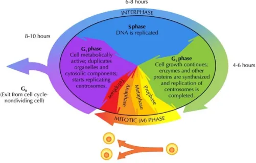
1.5 Cell cycle

The cell cycle is an ordered set of events that take place in a cell leading to its division and duplication. In cells with a nucleus the cell cycle can be divided in three periods: quiescent (G0 phase), interphase and the mitotic phase:

• The G0 phase is a resting phase where the cell has left the cycle and has stopped dividing.

• In the interphase, the cell is constantly synthesizing RNA, producing proteins and growing in size. Interphase can be divided into 3 steps: Gap 1 (G1), S (synthesis) phase, Gap 2 (G2).

– The G1 phase: Cells increase in size in Gap 1, produce RNA and synthesize proteins. An important cell cycle control mechanism ac-tivated during this period (G1 Checkpoint) ensures that everything is ready for DNA synthesis.

– The S phase: To produce two similar daughter cells, the complete DNA instructions in the cell must be duplicated. DNA replication occurs during this S (synthesis) phase.

(32)

• The mitotic phase consists of nuclear division. Cell growth and protein production stop at this stage in the cell cycle. All of the cell’s energy is focused on the complex and orderly division into two similar daughter cells. Mitosis is much shorter than interphase, since it is a relatively short period of the cell cycle. There is a Checkpoint in the middle of mitosis (Metaphase Checkpoint) that ensures the cell is ready to complete cell division.

Figure 1.4 shows a schematic view of the cell cycle.

Figure 1.4: Phases of the cell cycle. Figure reprinted with permission by Siyavula Education and made available at www.everythingscience.co.za

under the terms of a CC-BY 3.0 license [60].

1.6 Cell pathways

(33)

1.6. Cell pathways 11

Figure 1.5: The PI3K/Akt/mTOR signaling pathway [54]. This pathway is up-regulated in a significant proportion of ovarian cancers. Figure reprinted with permission from InTech.

Many solid cancers exhibit a deregulation of different oncogenic pathways. In the last years, many genes responsible for the genesis of different cancers have been discovered, their mutations identified, and the pathways through which they act characterized. A single mutated protein in a pathway can cause uncontrolled growth and cause cancer. “Targeted” cancer drugs are designed to block abnormal pathways. By blocking an overactive pathway, the drugs can slow a cancer’s growth and order malignant cells to self-destruct. Unfortunately, cancer cells can “learn” to activate other pathways, so that the original target drug is no longer effective by itself. Thus, the next step is to try to fight back by using combinations of drugs that attack multiple broken pathways.

(34)

downstream effects such as activating mTOR which regulates cell growth by controlling mRNA translation, ribosome biogenesis, autophagy, and metabol-ism [35]. Several studies have identified this pathway as the most frequently altered in different types of cancer [45][75][100].

As we indicated in the subsections about motivation and hallmarks, a hall-mark is an abstraction which can be activated as consequence of different malfunctions in the components of a pathway or pathways. Since our aims are focused on the study of the multicellular system behavior depending on the hallmarks acquired in the cells we will not consider the details of genes and proteins in the associated pathways.

1.7 Cancer stem cells

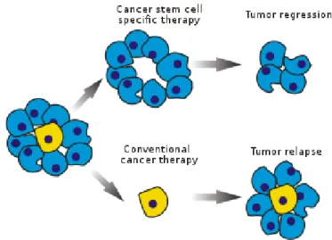
The cancer stem cell theory suggests that tumor cells include a minority popu-lation of cells responsible for the initiation of tumor development, growth, and tumor’s ability to metastasize and reoccur [25][34]. Cancer stem cells (CSCs) are cancer cells that possess features associated with normal stem cells, spe-cifically the ability to give rise to all cell types found in a particular cancer sample. Such cells are proposed to persist in tumors as a distinct population and cause relapse and metastasis by giving rise to new tumors [8].

Therefore, development of specific therapies targeted at CSCs holds hope for improvement of survival and quality of life of cancer patients, especially for patients with metastatic disease. The existence of CSCs has several implica-tions in terms of future cancer treatment and therapies. These include disease identification, selective drug targets, prevention of metastasis, and develop-ment of new intervention strategies. Thus, different works tried to simulate their behavior, taking into account their main characteristics, such as their capacity to divide indefinitely [103]. If current treatments of cancer do not properly destroy enough CSCs, the tumor will reappear, so it is important to understand their behavior and effects.

There are two models when considering the origin of cancer cells: The hier-archical model assumes that tumors are originated from CSCs that give rise to progeny with self-limited proliferative capacity where most of the cells in the tumor are genetically homogeneous. The second model is the stochastic model or clonal evolution model, which postulates that tumorigenesis is a multi-step process that leads to progressively genetic alterations with the transformation of healthy cells into malignant phenotypes [104]. Thus, two models have been considered for explaining the origin of cancer cells: In the hierarchical CSC model, CSCs can divide either symmetrically to yield two CSCs, or asymmet-rically to produce a CSC and a non-stem cancer cell with limited proliferation capacity (Differentiated Cancer Cell, DCC). These concepts will be exposed in better detail in chapter 4.

(35)

1.8. Organization of the thesis 13

Figure 1.6: In the Cancer Stem Cell (CSC) model these cells can divide sym-metrically or asymsym-metrically to produce Differentiated Cancer Cells (DCCs) with limited proliferative capability.

1.8 Organization of the thesis

This thesis describes the cancer growth model developed and the analysis of the simulation results. In the following paragraphs a short summary of each chapter is provided.

Chapter 2 describes the event model used for simulating the behavior of the multicellular system through time. The simulation algorithm is explained and different exploratory initial simulations using the event model are presented.

In Chapter 3 the relevance of hallmarks is studied in different representative situations of the first phases of cancer growth. Moreover, potential behavior transitions in tumor growth dynamics are analyzed when a treatment is applied in different scenarios defined by the relative prevalence of different hallmarks. Chapter 4 focuses on the simulation of the behavior of cancer stem cells to inspect their capability of regeneration of tumor growth in different scenarios. The analyses of the capabilities of the hallmarks to promote tumor growth serve also to test their capabilities in a cancer stem cell context.

In Chapter 5 the effect of cancer treatments in a cancer stem cell context is analyzed. The application of a standard treatment in a cancer stem context has consequences on tumor regrowth behavior. Therefore, different strategies when a treatment is applied will be analyzed by taking into account the implications of CSC presence.

In Chapter 6 evolutionary computing is used to optimize a treatment in terms of intensity, duration and periodicity taking into account the presence and effects of cancer stem cells. We selected for our objective Differential Evolution as a robust evolutionary method.

(36)

(37)

Chapter 2

Event model for tumor growth

simulation

2.1 Event model

We used an event model for simulating the behavior of the multicellular sys-tem through time, which is oriented to the modeling of the cell cycle taking into account the presence of the hallmarks in the cells. We used the event model introduced by Abbott et al. [1], which uses an event queue for storing possible future mitotic events. Moreover, each cell resides in a site in a 3D grid environment. In the modeling, each cell genome indicates if any hallmark is activated as consequence of mutations.

On the contrary to Abbott et al.’s work [1], in our case metastasis and angiogenesis are not considered, as we are interested in the first avascular phases of tumorigenesis. So, every cell has its “genome” which consists of five hallmarks with a binary representation indicating if each one of the hallmarks (Self Growth-SG, Ignore Growth Inhibit-IGI, Evade Apotosis-EA, Effective Inmortality-EI and Genetic Instability-GI) is activated, in addition to some parameters particular to each cell. These parameters are related with each of the hallmarks considered and the behavior of the cells when the hallmarks are acquired in a cell.

The parameters are briefly defined in Table 2.1, whereas in next subsections the implications of the parameters in the multicellular system behavior will be explained.

(38)

16 Chapter 2. Event model for tumor growth simulation

Table 2.1: Definition of the parameters associated with the hallmarks

Parameter name Default

value Description

Grid size The number of cells in the 3D lattice for the simulation.

Hallmark mutation rate (1/m) 10

5 Each gene (hallmark) is mutated (when the

cell divides) with a 1/mchance of mutation.

Telomere length

(tl) 50

Initial telomere length in each cell. Every time a cell divides, the length is shortened by one unit. When it reaches 0, the cell dies, unless the hallmark EI is ON.

Evade apoptosis (e) 10

A cell withnhallmarks mutated has an extra

n/e likelihood of dying each cell cycle, unless the hallmark EA is ON.

Genetic instability

(i) 10

2

There is an increase of the hallmark mutation rate by a factor ofifor cells with this mutation (GI).

Ignore growth in-hibit (g) 30

Cells with the hallmark “Ignore growth hibit” (IGI) activated have eliminated the in-hibition by contact. For the modeling, as in [1][94], these cells have a probability 1/g of killing off or replacing a neighbor to make room for mitosis.

Random cell death

(a) 10

3 In each cell cycle every cell has a 1/a chance

(39)

2.1. Event model 17 occasionally introduces a mutation that will be inherited by daughter cells. Then, at the G2 checkpoint, cells undergo a check for genetic damage. Apop-tosis is triggered in cells found to contain genetic defects. The G1 checkpoint is not modeled separately, because it is similar (This checkpoint prevents prepar-ation for DNA replicprepar-ation until the detected DNA damage has been removed). Finally, the cell undergoes mitosis in the M phase. One of the daughter cells occupies the grid location of its parent, while the other fills an empty adjacent location.

Algorithm 2.1.1 summarizes the simulation, which takes into account the main aspects of the cell cycle from the application point of view, specifying the order for testing the implications of the different hallmarks in the simulated cell cycle (TESTS 1 to 5).

Figure 2.1 represents graphically the algorithm in order to explain the procedure more clearly. The process is simulated as a event model where a mitosis is scheduled several times in the future, being a random variable distributed uniformly between 5 and 10 time steps (see Figure 2.2). This is done to simulate the variable duration of the cell life cycle (between 15 and 24 hours). Taking into account these time intervals, each time iteration represents an average time of 2.6 hours, so, for example, 5000 iterations in the simulation imply an average time of 77.4 weeks (1.48 years). Moreover, in the simulation, a grid with 106 sites represents approximately 0.1 mm3 of tissue. The main aspects of the model can be summarized in the following steps:

Start: The simulation can begin by initializing all elements of the grid to represent empty space, as in most previous works [1][11][25][80]. Then, the element at the center of the grid is changed to represent a single normal cell (no mutations). Mitosis is scheduled for this initial cell (push a mitotic event in the event queue between 5 and 10 time iterations in the future).

After the new daughter cells are created, mitoses are scheduled for each of them, and so on. Each mitotic division is carried out by copying the genetic information (the hallmark status and associated parameters) of the cell to an unoccupied adjacent space in the grid (a random free site among the 26 immediate neighbors in the 3D grid). Random errors occur in this copying process, so some hallmarks can be activated, taking into account that once a hallmark is activated in a cell, it will be never repaired by another mutation [1].

As an alternative, we will consider in our simulations an initial grid full of healthy cells, being the process the same but scheduling the mitoses for all the cells.

Pop event: The events are ordered on event time. Pop event from the event queue with the highest priority (the nearest in time) (see Figure 2.2).

(40)

Genetic damage test (Test 2): The larger the number of hallmark mutations, the greater the probability of cell death. If “Evade apoptosis” (EA) is ON, death as consequence of the genetic damage is not applied. This corresponds with the G2 checkpoint of the cell cycle (see Section 1.5).

Mitosis tests:

1. Replicative potential checking(Test 3): If the telomere length is 0, the cell dies, unless the hallmark “Effective immortality” (Limitless replicative potential, EI) is mutated (ON).

2. Growth factor checking (Test 4): As in [1][11][94], cells can per-form divisions only if they are within a predefined spatial boundary, which represents a threshold in the concentration of growth factor; beyond this area (95% of the inner space in each dimension in our simulations, which represents 85.7% of the 3D grid inner space) growth signals are too faint to prompt mitosis (unless hallmark SG is ON).

3. Ignore growth inhibit checking(Test 5): If there are not empty cells in the neighborhood, the cell cannot perform a mitotic division. As in [1][94], if the “Ignore growth inhibit” hallmark (IGI) is ON, then the cell competes for survival with a neighbor cell and with a likelihood of success (1/g).

If the three tests indicate possibility of mitosis:

• Increase the hallmark mutation rate if genetic instability (GI) is ON. That is, if the cell has this factor (GI) acquired then its mutation rate is increase by a factor (i).

• Add mutations to the new cells according to the hallmark mutation rate (1/m).

• Decrease telomere length in both cells.

• Push events. Schedule mitotic events (push in event queue) for both cells: Mother and daughter, with the random times in the future.

If mitosis cannot be applied:

• Schedule a mitotic event (in queue) for mother cell.

2.1.1 Comments about hallmark parameters

(41)

2.1. Event model 19

Algorithm 2.1.1: _{Event model for cancer simulation}()

t←0 //Simulation time. Initial cell at the centre of the grid.

Schedule a Mitotic Event(5,10)//Schedule a mitotic event with a //random time (ts) between 5 and 10 time iterations in the future //(t+ts). The events are stored in an event queue. The events are //ordered on event time.

whileevent in the event queue

do

Pop event( )//Pop event with the highest priority (the nearest in time). t← popped event time

TEST 1: Random cell death( )//The cell can die with a given //probability.

TEST 2: Genetic damage( )//The larger the number of hallmark //mutations, the greater the probability of cell //death. If “Evade apoptosis” (EA) is ON, death //is not applied.

Mitosis tests( ) :

TEST 3: Limitless replicative potential checking( )//If //the telomere length is 0, the cell dies, unless the hallmark

//“Effective immortality” (Limitless replicative potential, EI) is ON.

TEST 4: Growth factor checking( )//Cells can perform //divisions only if they are within a predefined spatial boundary which //sufficient growth factor; beyond this area cells cannot perform //mitosis, unless the hallmark “Self-growth” (SG) is ON.

TEST 5: Ignore growth inhibit checking( )//If there are not //empty cells in the neighborhood, the cell cannot perform a mitotic //division. If the “Ignore growth inhibit” hallmark (IGI) is ON, then //the cell can perform the division with a given probability, replacing //one of the neighbor cells.

if the three tests indicate possibility of mitosis

then

//Increase the hallmark mutation rate if “Genetic instability” //(GI) is ON.

//Add mutations to the new cells according to the hallmark //mutation rate (1/m). Decrease telomere length in both cells.

Push events( )

//Schedule mitotic events (push in event queue) for both cells: //mother and daughter, with the random times in the future.

(42)

Figure 2.1: Diagram of the event model. The rectangles indicate an action, a rhomb indicates a check with an associated binary question, as explained in the text. This process is repeated to all the cells in the grid environment. Each cell is represented with a small circle. If the cell dies after a check it is represented with a crossed-circle.

(43)

2.1. Event model 21 the simulations can use greater values of the initial telomere length -as in [1]-, being in this case the main limits for cell proliferation the area with growth factors and the grid size.

Other parameters are more difficult to determine in order to have a dir-ect analogy in nature. For example, as indicated by Spencer et al. [94], the parameters g, e and a were chosen via a sensitivity analysis such that the parameter plays an important role but does not dominate tumorigenesis or, as indicated in [1], the choice of parameter values “was guided by the obser-vation that hallmarks only have meaningful interactions within some region of interest”. We used a standard value of g= 30, a greater value than the one used in [1] (g= 10) and [94] (g= 5), implying a lower possibility of escaping the contact inhibition mechanism, although we will reason about the resultant behavior with different values.

The parameterm determines the probability of acquisition of a hallmark when the cell divides (hallmark mutation rate 1/m). Bielas et al. [13] de-veloped an assay to quantify random mutations in human tissue and their results showed that, in normal tissues, the frequency of spontaneous random mutations is exceedingly low, less than 10−8per base pair. In contrast, tumors exhibited an average frequency of 210·10−8 per base pair, an elevation of at least two orders of magnitude. Nevertheless, we must take into account that such values correspond to single-nucleotide mutations, while we are consider-ing mutations or acquisitions in the abstract model of the cancer hallmarks. Moreover, as indicated in [1], with small cell population sizes in the simula-tions, large mutation rates are necessary to obtain the expected incidence of cancer. So, we used the same default value considered in Abbott et al. [1] and Spencer et al. [94] for the probability of acquisition of hallmarks in the mitotic divisions. Also, Basanta et al. [11] worked with parameters, such as hallmark mutation rate (10−5_{) and mutation rate increase for cells with acquired genetic}

instability (i= 100), with the same default values.

For the grid size, we also used the same size of Abbot et al. [1] for most of the experiments (125000 cell sites). The reason is that “even with modern processor speeds, it is still not feasible to simulate a realistic number of cells using an individual-based approach in which each cell is represented explicitly” [1]. Moreover, as detailed in the next chapter, the emergent behavior will be independent of the grid size, provided that we use a sufficient number of cells to capture the emergent dynamics of the process with the interrelations of the hallmarks [65][85].

(44)

arbit-22 Chapter 2. Event model for tumor growth simulation

Figure 2.3: Self-Growth hallmark rule.

rary, as in the referenced works (Abbot et al. [1], Spencer et al. [94], Basanta et al. [11]), but reasonable to show the effect of the hallmark SG in such a stage. Changing the size of the area with growth factors would not change the conclusions, except that the situation when the system growth reaches the limits with growth factors would occur in a different time iteration.

Finally, in the simulation, there is not any boundary condition beyond the grid size and that the outer area of the grid is not filled with growth factor. That is, a cell cannot divide beyond the limits in each dimension and there are not neighborhood connections, for example, between the cells of the left-side limit and the right-side limit.

2.1.2 Hallmarks rules in a graphical way

As indicated in the simulation steps, frequently, cells are unable to replicate because of some limitation, such as contact inhibition or insufficient growth signal. Cells overcome these limitations through mutations in the different hallmarks. The different tests considered in the simulation of the mitotic and apoptotic behavior of the cells, taking into account the different hallmarks acquired, are a set of rules that are applied to each of the cells of the 3D envir-onment. Therefore, we are using the classical concept of a cellular automaton where the rules are applied to a cell of the grid-like environment when an event is popped from the event queue regarding that cell and site. Figures 2.3 to 2.7 show, in a schematic view, the implications of the rules of the cellular automaton.

(45)

2.1. Event model 23

Figure 2.4: Ignore Growth Inhibit hallmark rule.

(46)

Figure 2.6: Effective Immortality hallmark rule.

(47)

2.2. Examples of simulation runs 25 cell can perform mitosis out of the predefined area with growth factor. In the Figure an example in 2D is shown but in the simulation a 3D space is used.

In Figure 2.4 the rule of the hallmark ignore growth inhibit is explained. A normal cell cannot perform mitosis if there is no empty space in its neigh-borhood, unless the hallmark IGI is ON. In this last case, a neighbor is killed probabilistically to make room for mitosis. These cells (hallmark IGI ON) have a probability 1/gof replacing a neighbor, as indicated in Table 2.1.

Figure 2.5 explains the rule of the hallmark evade apoptosis. A cell with the hallmark EA activated does not die by apoptosis.

Figure 2.6 illustrates the rule regarding hallmarkeffective immortality. A normal cell dies when its telomere length (decreased in every cell division) reaches the value 0, but a cell with the hallmark EI activated can continue dividing indefinitely.

Finally, Figure 2.7 graphically explains the rule of the hallmark genetic instability. A cell with this hallmark activated increases the hallmark mutation rate by a factori, as indicated in Table 2.1.

2.2 Examples of simulation runs

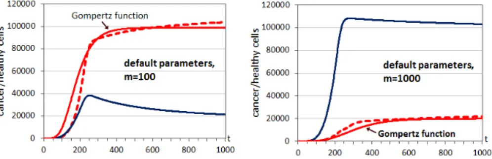
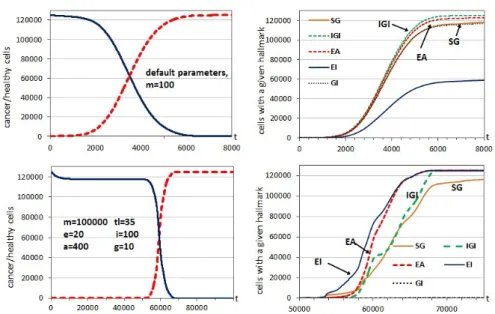
This section illustrates exploratory initial simulations using the event model explained. Figure 2.8 shows the evolution over time of the number of healthy and cancer cells for two different values of the parameter m, which defines the hallmark mutation rate, maintaining the rest of the parameters in their default values and using the same grid size (125000, grid with 50 sites in each dimension) employed in [1]. The number of time iterations was 1000 in the different runs. A cell was considered as cancerous if any of the hallmarks was present. As expected, with increasing hallmark mutation rates (1/m), the increase in cancer cells becomes faster. For lower values of the hallmark mutation rate it is difficult to obtain rapid cancer progression, so we selected those two high values.

(48)

Rodriguez-Brenes et al. [84] analyzed tumor growth patterns and they classified them into five fundamentally different categories:

• The exponential growth is the simplest model used to describe tumor growth. Several leukemias and lymphomas exhibited exponential growth, most notably the L1210 leukemia [90]. Exponential growth has also been documented to describe the growth dynamics of certain non-solid cancers [27], but this law is not applicable to most solid tumors over long time periods.

• The surface growth suggests a linear relation between time and the dia-meter of a tumor. The models that follow this pattern use the basic idea that most of the growth activity is concentrated at the boundary of the tumor (cells near the surface divide more often than the cells in the core).

• The Sigmoidal growth is comprised by three distinct phases: the ini-tial exponenini-tial phase, the linear phase, and the plateau where popula-tion size stabilizes (saturapopula-tion). If the growth rate decays exponentially, we get the Gompertz law [84]. There is empirical evidence that tumor growth follows a Gompertz function in a lot of cancer types. In the 1960s, A.K. Laird [50], for the first time, successfully used the Gompertz curve to fit the growth of 19 tumor lines (ten mice, eight rats, and one rabbit) using the following equation: V(t) = [V0eA/B(1−e

Bt

)_{] where V}

represents the tumor size, in appropriate units, at any time t, V0 is the

initial tumor size, and A and B are constants that vary depending on the type of cancer. Since then, this equation has been extensively used in this context.

• Atypical growth corresponds to other data sets, of solid and non-solid tumors, that do not conform to the growth laws described so far. These data sets show sub-cubic growth for solid tumors and sub-exponential growth for non-solid tumors.

• Multistep growth is an irregular growth pattern based on the idea that the development of cancer is a multistep process in which cells gradually become malignant through a progressive series of alterations (random mutations and epigenetic changes) [62][70]. An irregular pattern of tu-mor growth generally incorporates plateaus or dormant periods separ-ated by Gompertzian growth periods.

In the runs of Figure 2.8, using the standard parameters, the tumor growth follows a Gompertz curve since we have the three distinct phases: exponen-tial phase, the linear phase and the saturation. In this figure a Gompertz growth curve is included for comparison with respect to the growth curve of the simulations (cancer cells). Depending on the parameters of the simulation the different phases are more o less pronounced. The inserted curve with a Gompertz type growth in Figure 2.8 with m=100 has the following constants of the Gompertz function: V0=1, A=0,1845 and B=0,016. For the case of

(49)

(50)

(51)

Chapter 3

Relevance of hallmarks

In this chapter we study the evolution of hallmarks in different representat-ive situations of the first phases of cancer growth, regarding initial conditions and parameters, analyzing the relative importance of the hallmarks for tumor progression. The presence of the cancer hallmarks defines cell states and cell mitotic behaviors. As previously explained, these hallmarks are associated with a series of parameters, and depending on their values and the activation of the hallmarks in each of the cells, the system can evolve to different dynam-ics. Such possible dynamics are analyzed here. Moreover, we study possible behavior transitions in tumor growth dynamics when a treatment is applied in different scenarios defined by the relative predominance of different hallmarks.

3.1 Dependence on hallmark parameters

In this section we show the capability of the simulation tool for obtaining different dynamic behaviors. Figures 3.1, 3.2 and 3.3 (left part) show the evolution over time of the number of healthy and cancer cells for different values of the parameter m, which defines the hallmark mutation rate, maintaining the rest of the parameters in their default values and using the same grid size (125000). As in the previous initial examples in previous chapter, the simulations began with only one healthy cell at the center of the grid. A cell was considered cancerous if any of the hallmarks was present. The graphs are an average of 5 different runs, given the stochastic nature of the problem. The number of time iterations was 1000 in the different runs.

The central graphs of Figures 3.1, 3.2 and 3.3 show the time evolution of the cells with a given hallmark and such standard parameters. With the highest mutation rate (m= 100, Fig. 3.3), despite the rapid and initial cancer cell progression, two hallmarks present an advantage for cancer cell proliferation:

(52)

30 Chapter 3. Relevance of hallmarks

Figure 3.1: Left: Evolution through time iterations of the number of healthy cells (continuous line) and cancer cells (dashed line) withm= 10000 and para-meter default values. Center: Time evolution of the number of cells with a hallmark acquired. All the graphs are an average of 5 independent runs. Right: Example of a 2D cross-section of a final configuration at the end of the tem-poral evolution (att= 1000). Healthy cells are shown in bright gray whereas the other colors correspond to different combinations of hallmarks acquired.

except for those with hallmark IGI acquired (the free space limitation can be ignored by such cells). It should be remembered that these hallmarks, that allow the cells to escape those limits, are acquired by the offspring, so the daughters can continue proliferating. Using a lower hallmark mutation rate (m= 1000, Fig. 3.2), the hallmarkself-growth (SG) is initially more predom-inant than IGI, as cells with hallmark SG acquired proliferate rapidly when the cells have reached the limits of the area filled with growth factor. With the lowest mutation rate (m= 10000, Fig. 3.1), the hallmarkself-growth (SG) is the most predominant since, when the cells have reached the limits with growth factor, the cells with that mutation can proliferate rapidly in the small area without growth factor. In this case, the hallmarkevade apoptosis (EA) is less predominant, as there are fewer mutations in cells, so the apoptosis mechanism is less important as a limit to cell proliferation. Table 3.1 includes statistical information of these simulation runs, with the final information of healthy and cancer cells at the end of the simulation at t= 1000, to know the variability involved in the different runs. We must take into account that the variability depends on the particular iteration at which the simulation is ended. For example, with simulations that end with the whole grid practically full of one type of cells, the variability of the runs is logically lower (m= 10000 in Fig. 3.1).

(53)

di-3.1. Dependence on hallmark parameters 31

Figure 3.2: Left: Evolution through time iterations of the number of healthy cells (continuous line) and cancer cells (dashed line) with m= 1000 and para-meter default values. Center: Time evolution of the number of cells with a hallmark acquired. All the graphs are an average of 5 independent runs. Right: Example of a 2D cross-section of a final configuration at the end of the temporal evolution (at t= 1000).

Figure 3.3: Left: Evolution through time iterations of the number of healthy cells (continuous line) and cancer cells (dashed line) with m= 100 and para-meter default values. Center: Time evolution of the number of cells with a hallmark acquired. All the graphs are an average of 5 independent runs. Right: Example of a 2D cross-section of a final configuration at the end of the temporal evolution (at t= 1000).

vision), so there are clusters of concentrated or localized cells with hallmarks acquired.

TítuloTumor growth analysis using cellular automata based on the cancer hallmarks

Departamento de Computaci´

on

Tumor growth analysis using cellular automata

based on the cancer hallmarks

PhD Thesis

Tese de doutoramento

´

Angel Monteagudo Insua

PHD THESIS

Tumor growth analysis using cellular

automata based on the cancer hallmarks

´

Angel Monteagudo Insua

PhD supervisor:

Dr. Jos´e Santos Reyes

Thesis committee:

Dr. Amparo Alonso Betanzos

Dr. Rafael Lahoz Beltr´

a

D. Jos´

e Santos Reyes

, Profesor Titular de Universidad en el ´

area

de Ciencias de la Computaci´

on e Inteligencia Artificial de la

Uni-versidade da Coru˜

na

CERTIFICA

Que la presente memoria titulada

Tumor growth analysis

us-ing cellular automata based on the cancer hallmarks

fue realizada

bajo su direcci´

on y constituye la Tesis que presenta

D. ´

Angel

Mon-teagudo Insua

para optar al grado de Doctor por la Universidade

da Coru˜

na.

A Coru˜

na, diciembre de 2015

Acknowledgments

Abstract

Table of contents

List of Tables

List of Figures

Chapter 1

Introduction

1.1

Motivation

1.2

Previous works using cellular automata for

tu-mor growth modeling

1.3

The biology of cancer

1.4

The hallmarks of cancer

1.5

Cell cycle

1.6

Cell pathways

1.7

Cancer stem cells

1.8

Organization of the thesis

Chapter 2

Event model for tumor growth

simulation

2.1

Event model

2.1.1

Comments about hallmark parameters

2.1.2

Hallmarks rules in a graphical way

2.2

Examples of simulation runs

Chapter 3

Relevance of hallmarks