Chaos in King's iterative family

Texto completo

(1)Título artículo / Títol article:. Chaos in King's iterative family. Autores / Autors. A. Cordero; Javier Garcia‐Maimó; Juan R. Torregrosa; María P. Vassileva; Pura Vindel. Revista:. Applied Mathematics Letters, v. 26, issue 8 (August 2013). Versión / Versió:. Preprint de l’autor. Cita bibliográfica / Cita bibliogràfica (ISO 690):. Cordero, A.; García-Maimó, Javier; Torregrosa, Juan R; Vassileva, Maria P.; Vindel, Pura. Chaos in King's iterative family. Applied Mathematics Letters, v. 26, issue (2013), p. 842-848. url Repositori UJI:. http://repositori.uji.es/xmlui/handle/10234/90096.

(2) familia_king_aml.tex Click here to view linked References. Chaos in King’s iterative family ✩ Alicia Corderoa,∗, Javier Garcı́a-Maimób, Juan R. Torregrosaa, Maria P. Vassilevab , Pura Vindelc a Instituto. Universitario de Matemática Multidisciplinar Universitat Politècnica de València Camino de Vera s/n, 46022 València, Spain b Instituto Tecnológico de Santo Domingo Santo Domigo, Dominican Republic c Instituto de Matemáticas y Aplicaciones de Castellón Universitat Jaume I Campus de Riu Sec s/n, Castellón, Spain. Abstract In this paper, the dynamics of King’s family of iterative schemes for solving nonlinear equations is studied. The parameter spaces are presented, showing the complexity of the family. The analysis of the parameter space allows us to find elements of the family that have bad convergence properties, and also other ones with stable behavior. Keywords: Nonlinear equations; Iterative methods; Dynamical behavior; Quadratic polynomials; Fatou and Julia sets; King’s family; Non-convergence regions.. 1. Introduction The application of iterative methods for solving nonlinear equations f (z) = 0, with f : C → C, gives rise to rational functions whose dynamics are not well-known. From the numerical point of view, the dynamical behavior of the rational function associated with an iterative method give us important information about its stability and reliability. In these terms, Varona in [1] and Amat et al. in [2] described the dynamical behavior of several well-known iterative methods. More recently, in [3, 4, 5, 6, 7, 8, 9], the authors study the dynamics of different iterative families. In most of these studies, interesting dynamical planes, including some periodical behavior and other anomalies, have been obtained. However, in contrast to dynamical planes, the parameter planes associated to a family of methods allow us to understand the behavior of the different members of the family of methods, helping us in the election of a particular one. The family under study is, in this case, King’s family of iterative methods (see [10]). It is an uniparametric set of fourth-order iterative schemes to estimate simple roots of nonlinear equations f (z) = 0: zk+1 = yk − where yk = zk −. f (zk ) + (2 + β)f (yk ) f (yk ) , k = 0, 1, . . . , f (zk ) + βf (yk ) f " (zk ). (1). f (zk ) and β is a parameter. This family includes the known Ostrowski’s method for β = −2 (see f " (zk ). [11]). In [12], the authors described the conjugacy classes of King’s iterative methods and made an excellent initial analysis of their dynamics when they are applied to generic low-degree polynomials. In this work, we deep in the study of the dynamics of this set of methods when they are applied to quadratic polynomials, characterizing completely the stability of all the fixed points. It is known that the roots of a polynomial can be transformed by an affine map with no qualitative changes on the dynamics of family (1) (see [12]). So, we can use the quadratic polynomial p (z) = z 2 + c. For p(z), the operator of the ✩ This research was supported by Ministerio de Ciencia y Tecnologı́a MTM2011-28636-C02-02 and FONDOCYT 2011-1-B1-33 República Dominicana. ∗ Corresponding author Email addresses: [email protected] (Alicia Cordero ), [email protected] (Javier Garcı́a-Maimó), [email protected] (Juan R. Torregrosa), [email protected] (Maria P. Vassileva), [email protected] (Pura Vindel). Preprint submitted to Elsevier. February 13, 2013.

(3) family corresponds to the rational function: Kp,β (z) =. c3 (2 + β) + 3cz 4 (10 + β) + z 6 (10 + 3β) − c2 z 2 (10 + 7β) , 8z 3 (−cβ + z 2 (4 + β)). depending on the parameters β and c. P. Blanchard, in [13], by considering the conjugacy map √ z−i c √ , h (z) = z+i c. (2). with the following properties: i) h (∞) = 1,. !√ " ii) h i c = 0,. ! √ " iii) h −i c = ∞,. proved that, for quadratic polynomials, the Newton’s operator is always conjugate to the rational map z 2 . In an analogous way, the operator Kp,β on quadratic polynomials is conjugated to the operator Oβ (z), ! " 5 + 4z + z 2 + β(2 + z) Oβ (z) = h ◦ Kp,β ◦ h−1 (z) = z 4 . 1 + (4 + β)z + (5 + 2β)z 2. (3). We observe that the parameter c has been obviated in Oβ (z). We will study the general convergence of methods (1) for quadratic polynomials. To be more precise (see [14, 15]), a given method is generally convergent if the scheme converges to a root for almost every starting point and for almost every polynomial of a given degree. Now, we are going to recall some dynamical concepts of complex dynamics (see [16]) that we use in this work. Given a rational function R : Ĉ → Ĉ, where Ĉ is the Riemann sphere, the orbit of a point z0 ∈ Ĉ is defined as: {z0 , R (z0 ) , R2 (z0 ) , ..., Rn (z0 ) , ...}. We analyze the phase plane of the map R by classifying the starting points from the asymptotic behavior of their orbits. A z0 ∈ Ĉ is called a fixed point if R (z0 ) = z0 . A periodic point z0 of period p > 1 is a point such that Rp (z0 ) = z0 and Rk (z0 ) '= z0 , for k < p. A pre-periodic point is a point z0 that is not periodic but there exists a k > 0 such that Rk (z0 ) is periodic. A critical point z0 is a point where the derivative of the rational function vanishes, R" (z0 ) = 0. Moreover, a fixed point z0 is called attractor if |R" (z0 )| < 1, superattractor if |R" (z0 )| = 0, repulsor if |R" (z0 )| > 1 and parabolic if |R" (z0 )| = 1. The basin of attraction of an attractor α is defined as: A (α) = {z0 ∈ Ĉ : Rn (z0 ) →α, n→∞}. The Fatou set of the rational function R, F (R) , is the set of points z ∈ Ĉ whose orbits tend to an attractor (fixed point, periodic orbit or infinity). Its complement in Ĉ is the Julia set, J (R). That means that the basin of attraction of any fixed point belongs to the Fatou set and the boundaries of these basins of attraction belong to the Julia set. The rest of the paper is organized as follows: in Section 2 we analyze the fixed and critical points of the operator Oβ (z) and in Section 3 we study the stability of the fixed points. The dynamical behavior of the family (1) is analyzed in Section 4, by using one of the associated parameter spaces. We finish the work with some remarks and conclusions. 2. Analysis of the fixed and critical points The fixed points of Oβ (z) are the roots of the equation Oβ (z) = z, that is, z = 0, z = ∞ and the strange fixed points • z = 1 for β '=. −10 3 ,. + β) − 14 B1 −. 1 2. # −12 − 3β + (1/2)(5 + β)2 − B2 , # 1 1 −12 − 3β + (1/2)(5 + β)2 − B2 , • ex2 = −1 4 (5 + β) − 4 B1 + 2 # 1 1 −12 − 3β + (1/2)(5 + β)2 + B2 , • ex3 = −1 4 (5 + β) + 4 B1 − 2 # 1 1 • ex4 = −1 −12 − 3β + (1/2)(5 + β)2 + B2 , 4 (5 + β) + 4 B1 + 2 • ex1 =. −1 4 (5. 2.

(4) # where B1 = β 2 − 2β − 7 and B2 = (−1/2)(5 + β)B1 . Some relations between the strange fixed points are described in the following lemma. Lemma 1. The number of simple strange fixed points of operator Oβ (z) is five, except in cases: i) If β = −2, then ex1 = ex2 = −1. So, there exist 4 strange fixed points, one of them with multiplicity two. ii) If β =. −10 3 ,. there are four simple strange fixed points. √ iii) When β = 1 ± 2 2, ex1 = ex3 and ex2 = ex4 . There are only 3 strange fixed points, two of them double. iv) If β = −22/5, then ex3 = ex4 = 1 and there are two simple strange points and a triple one. v) Moreover, if β = −5, then ex1 = −ex4 and ex2 = −ex3 , and vi) if β = −8/3, then ex3 = −ex4 . In order to determine the critical points, we calculate the first derivative of Oβ (z), Oβ" (z) = 2z 3 (1 + z)2. 10 + 4β + 20z + 14βz + 3β 2 z + 10z 2 + 4βz 2 . (1 + 4z + βz + 5z 2 + 2βz 2 )2. A classical result establishes that there is at least one critical point associated with each invariant Fatou component. It is clear that the roots of the polynomial, z = 0 and z = ∞, are critical points and give rise to their respective Fatou components, but there exist in the family some free critical points, that is, critical points different from the roots, some of them depending on the value of the parameter. Lemma 2. Analyzing the equation Oβ" (z) = 0, we obtain a) If β = −2, there is no free critical points of operator Oβ (z). b) If β = −5/2 or β = 0, then z = −1 is the only free critical point. c) In any other case, (i) z = −1 (ii) cr1 = (iii) cr2 =. −20−14β−3β 2 − −20−14β−3β 2 +. √. 3β(β+2)(β+4)(3β+10) 4(2β+5). √. 3β(β+2)(β+4)(3β+10) 4(2β+5). =. 1 cr1. are free critical points. Some of these properties determine the complexity of the operator, as we can see in the following result. Theorem 1. The only member of King’s family whose operator is always conjugated to the rational map z 4 is Ostrowski’s method. Proof. From (3), we denote p(z) = z 2 + (4 + β)z + (5 + 2β) and q(z) = (5 + 2β)z 2 + (4 + β)z + 1. By factorizing both polynomials, we can observe that the unique value of β verifying p(z) = q(z) is β = −2. From the previous results, let us remark that • At most, there are only two different free critical points. • When β =. −10 3 ,. cr1 = cr2 = 1 that is not a fixed point, and the associated operator is Oβ (z) = z 4 z+5/3 z+3/5 .. 5 z+3/2 • If β = −5 2 , then the associated operator is Oβ (z) = z 3/2z+1 . So, for quadratic polynomials, the corresponding method has order of convergence five.. • if β = −4, then cr1 = cr2 = 1 that is an strange fixed point. As we will see in the following section, not only the number but also the stability of the fixed points depend on the parameter of the family.. 3.

(5) 3. Stability of the fixed points It is clear that the origin and ∞ are always superattractive fixed points, but the stability of the other fixed points changes depending on the values of the parameter β. In the following results we establish the stability of the strange fixed points. Theorem 2. The character of the strange fixed point z = 1 is: $ $ 16 $ i) If $β + 226 55 < 55 , then z = 1 is an attractor and it is a superattractor if β = −4. $ 16 $ $ ii) When $β + 226 55 = 55 , z = 1 is a parabolic point. $ $ 16 $ iii) If $β + 226 55 > 55 , then z = 1 is a repulsor.. Proof. It is easy to proof that. Oβ" (1) = So,. $ $ $ 8(4 + β) $ $ $ $ 10 + 3β $ ≤ 1. 8(4 + β) . 10 + 3β. is equivalent to. 8 |4 + β| ≤ |10 + 3β| .. Let us consider β = a + ib an arbitrary complex number. Then, ! " 82 162 + 8a + a2 + b2 ≤ 100 + 60a + 9a2 + 9b2 . By simplifying. 55a2 + 55b2 + 452a + 924 ≤ 0, that is,. &2 % &2 % 16 226 2 +b ≤ . a+ 55 55. Therefore,. $ $ $ " $ $ $ $Oβ (1)$ ≤ 1 if and only if $β + 226 $ ≤ 16 . $ 55 $ 55 $ $ $ 16 $ $ " $ $ Finally, if β satisfies $β + 226 55 > 55 , then $Oβ (1)$ > 1 and z = 1 is a repulsive point. Similar results can be proved for the rest of strange fixed points. Theorem 3. The real analysis of the stability of strange points ex1 and ex2 shows that: √ √ i) If β ∈] − 1.83917, 1 − 2 2[∪]1 + 2 2, 3.96186[, then both points are attractors and they are superattractors when β ≈ −1.83192 and β ≈ 3.86866. √ ii) If β = 1 ± 2 2, β ≈ −1.83917 or β ≈ 3.96186, then ex1 and ex2 are parabolic. iii) In any other case, both are repulsors. Theorem 4. The stability of ex3 and ex4 for real values of β verify: i) If β ∈] − 4.97983, −22/5[, then ex3 and ex4 are attractors, and superattractors if β ≈ −4.7034. √ ii) When β = 1 ± 2 2, β = −22/5 or β ≈ −4.97983, they are parabolic. iii) In any other case, both are repulsors. In Figure 1, we show the behavior of the strange and critical points for real values of β.. 4.

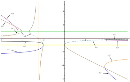
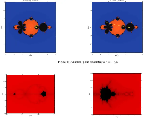
(6) 4 ex4. 2. cr1 ex3. ex2. cr2 !6. !4. 2. !2 ex2. 4. 6. cr2. ex4. ex1 !2 ex3. !4. ex1. !6. Figure 1: Bifurcation diagram of fixed and critical points. 4. The parameter space The dynamical behavior of operator Oβ (z) depends on the values of the parameter β. The parameter space associated with a free critical point of family (1) is obtained by associating each point of the parameter plane with a complex value of β, i.e., with an element of family (1). Every value of β belonging to the same connected component of the parameter space give rise to subsets of schemes of family (1) with similar dynamical behavior. So, it is interesting to find regions of the parameter plane as much stable as possible, because these values of β will give us the best members of the family in terms of numerical stability. As cr1 = cr12 , we have at most two free critical points, so we can obtain different parameter planes, with complementary information. When we consider the free critical point z = −1 as a starting point of the iterative scheme of the family associated to each complex value of β, we paint this point of the complex plane in red if the method converges to any of the roots (zero and infinity) and they are black in other cases. Then, the parameter plane P1 is obtained; it is showed in Figure 2. −3. −0.5 −2. IIm{c}. IIm{c}. −1. 0. 0. 1. 2. 0.5 −5.5. 3. −5. −4.5 IRe{c}. −4. −6. −3.5. −4. −2. 0. 2. 4. IRe{c}. Figure 3: Parameter space P2 associated to z = cri , i = 1, 2. Figure 2: Parameter plane P1 associated to z = −1. A similar procedure can be carried out with the free critical points, z = cri , i = 1, 2, obtaining the same parameter space P2 , showed in Figure 3. In the left of this parameter space we observe a black figure with a certain similarity with the known Mandelbrot set (see [17]) that we call the mask. In the following, we will focus our attention on parameter plane P2 . In the mask, we observe two large disks (the right disk is denoted by D1 and the left one by D2 ): D1 corresponds to values of β for which z = 1 is attractive or superattractive (see Theorem 2) and D2 is the region where strange fixed points ex3 and ex4 are attractive or superattractive (see Theorem 4). In Figure 4, the dynamical plane of the iterative method corresponding to β = −4.5 is presented, showing the existence of four different basins of attraction, two of them of the superattractors 0 and ∞ and the other two corresponding the atractors ex3 and ex4 . Other regions of the parameter plane P2 with stability problems are the right central and outer antennas, where Mandelbrot sets appear, corresponding to the stability regions of ex1 and ex2 (Theorem 3). A detail of these region is presented in Figure 5. 5.

(7) Figure 4: Dynamical plane associated to β = −4.5. −0.3 −0.06. −0.2. −0.04. −0.1. IIm{c}. IIm{c}. −0.02. 0. 0.02. 0.1. 0.04. 0.06 −1.95. 0. 0.2. −1.9. −1.85. −1.8. 0.3. IRe{c}. 3.7. 3.8. 3.9. 4. 4.1. 4.2. 4.3. 4.4. IRe{c}. Figure 5: Details of the right central and outer antennas of P2. A particular value of β in this region is β = 3.9 + 0.1i. It is placed in a bulb around the Mandelbrot set. The corresponding dynamical plane is showed in Figure 6. We can observe the existence of three basin of attraction, two of them associated to the roots and the other to an attracting periodic orbit of period 3, {−4.5579 + i0.37156, −4.4582 + i0.05353, −4.7681 + i0.27481}. Sharkovsky’s Theorem ([17]), states that the existence of orbits of period 3, guaranties orbits of any period. Cases β = −4.5 and β = 3.9 + 0.1i are only two of many situations that highlight the dynamical wealth of this family and also that the analysis of parameter planes are a useful tool for its study. 5. Conclusions The dynamical behavior of King’s family is very rich. It has been proved that there are many regions with no convergence to the roots, and the existence of periodic orbits of arbitrary period has been showed. Nevertheless, there are wide regions in parameter space whose corresponding iterative methods have a a good numerical behavior, in terms of stability and efficiency even in terms of order, as β = −5 2 . These regions are associated to non-black regions in both parameter planes simultaneously. Interesting future studies deal with the interaction between free critical points in black regions of P1 and P2 . 6. References References [1] J.L. Varona, Graphic and numerical comparison between iterative methods, Math. Intelligencer 24(1) (2002) 37-46. [2] S. Amat, S. Busquier, S. Plaza, Review of some iterative root-finding methods from a dynamical point of view, Scientia Series A: Mathematical Sciences 10 (2004) 3-35.. 6.

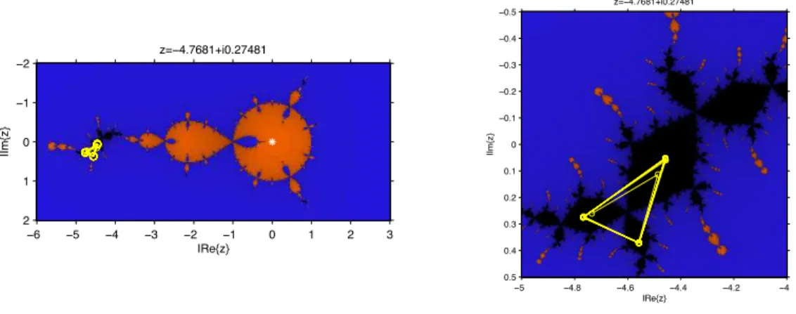
(8) z=−4.7681+i0.27481 −0.5 −0.4. z=−4.7681+i0.27481 −2. −0.3 −0.2. −1 IIm{z}. IIm{z}. −0.1. 0. 0 0.1. 1 0.2. 2 −6. 0.3. −5. −4. −3. −2. −1 IRe{z}. 0. 1. 2. 3 0.4 0.5 −5. −4.8. −4.6. −4.4. −4.2. −4. IRe{z}. Figure 6: Periodic orbit for β = 3.9 + 0.1i. [3] J.M. Gutiérrez, M.A. Hernández and N. Romero, Dynamics of a new family of iterative processes for quadratic polynomials, J. of Computational and Applied Mathematics 233 (2010) 2688-2695. [4] G. Honorato, S. Plaza, N. Romero, Dynamics of a high-order family of iterative methods, Journal of Complexity 27 (2011) 221-229. [5] F. Chicharro, A. Cordero, J.M. Gutiérrez, J.R. Torregrosa, Complex dynamics of derivative-free methods for nonlinear equations, Applied Mathematics and Computation doi: 10.1016/j.amc.2012.12.075. [6] S. Artidiello, F. Chicharro, A. Cordero, J.R. Torregrosa, Local convergence and dynamical analysis of a new family of optimal fourth-order iterative methods, International Journal of Computer Mathematics doi:10.1080/00207160.2012.748900. [7] M. Scott, B. Neta, C. Chun, Basin attractors for various methods, Applied Mathematics and Computation 218 (2011) 2584-2599. [8] C. Chun, M.Y. Lee, B. Neta, J. Džunić, On optimal fourth-order iterative methods free from second derivative and their dynamics, Applied Mathematics and Computation 218 (2012) 6427-6438. [9] B. Neta, M. Scott, C. Chun, Basin attractors for various methods for multiple roots, Applied Mathematics and Computation 218 (2012) 5043-5066. [10] R. F. King, A family of fourth-order methods for nonlinear equations, SIAM J. Numer. Anal. 10 (5) (1973) 876-879. [11] A.M. Ostrowski, Solution of equations and systems of equations, Prentice-Hall, Englewood Cliffs, NJ, USA, 1964. [12] S.Amat, S.Busquier, S. Plaza, Dynamics of the King and Jarratt iterations, Aequationes Math. 69 (2005) 212-223. [13] P. Blanchard, The Dynamics of Newton’s Method, Proc. of Symposia in Applied Math. 49 (1994) 139-154. [14] S. Smale, On the efficiency of algorithms of analysis, Bull. Allahabad Math. Soc. 13 (1985) 87-121. [15] C. McMullen, Family of rational maps and iterative root-finding algorithms, Ann. of Math. 125 (1987) 467-493. [16] P. Blanchard. Complex Analytic Dynamics on the Riemann Sphere, Bull. of the AMS 11(1) (1984) 85-141. [17] R.L. Devaney, The Mandelbrot Set, the Farey Tree and the Fibonacci sequence, Am. Math. Monthly 106(4) (1999) 289-302.. 7.

(9)