Estimating the environmental Kuznets curve for Spain by considering fuel oil prices (1874–2011)

Texto completo

(1)Estimating the environmental Kuznets curve for Spain by considering fuel oil prices (1874-2011) a. Jacint Balaguera and Manuel Cantavellaa Department of Economics and International Economics Institute, UniversitatJaume I, Campus Riu Sec, 12071 Castellón, Spain.. Abstract We perform a structural analysis on an environmental Kuznets curve (EKC) for Spain by exploiting long time series (1874-2011) and by using real oil prices as indicator of variations in fuel energy consumption. This empirical strategy allows us to both, capture the effect of the most pollutant energy on carbon dioxide (CO2) emissions and, at the same time, preclude potential endogeneity problems derived from the direct inclusion of fuel consumption in econometric specification. Knowingthe extent to whichoil prices affect CO2 emissions has a straightforward application for environmental policy. The dynamics estimates of the long and short-term relationships among CO2, economic growth and oil prices, are built through an autoregressive distributed lag (ARDL) model. Our test results support the EKC hypothesis. Moreover, real oil prices are clearly revealed as a valuable indicator of pollutant energy consumption. Keywords Environmental Kuznets curve, CO2; Oil prices; Autoregressive distributed lag model; Time series.. 1. Introduction Over time, humankind has contributed to atmosphere contamination through different processes of production and consumption. From the seventies, when a major concern on the environment’s deterioration took place at international level, some.

(2) economists argued that enhancement in per capita income could eventually reduce the level of environment degradation. We can distinguish at least two arguments widely used to explain this possible phenomenon. That is, on the one hand, the variation towards a new productive structure which uses a lower level of polluting energies. On the other hand, the social willingness to pay for the extra cost associated to the cleaner energies. These underlying ideas were enthusiastically accepted when an early set of papers (e.g., Grossman and Krueger, 1991; Shafik and Bandyopadhyay, 1992; Panayotou, 1993) provided the first formal evidence about an inverted U-shape relationship between per capita income and environmental degradation following, therefore, a Kuznets type curve.1 Nowadays, we can appeal to many studies that show the existence of an environmental Kuznets curve (EKC) for several countries by using different sample periods, econometric modeling and empirical methods. With the aim of contributing to the knowledge on the EKC for CO2 emissions, this paper provides new evidence for Spain by exploiting time series from a large period (1874-2011). We will analyze the possible effect on Spanish CO2 emissions generated not only from economic growth but also from changes in pollutant energy consumption. However, the direct inclusion of pollutant energy consumption in models would introduce endogeneity problems since the available measures of CO2 are contemporaneously correlated with that variable. In fact, the Carbon Dioxide Information Analysis Center (CDIAC) calculates the total CO2 emissions by multiplying different primary energy sources (coal, petroleum, and natural gas) by their respective emission rates. Then, we will consider as an indicator of pollutant energy consumption real oil prices that, in turn, can be conformed as a useful instrument for environmental policy. 1. Kuznets (1955) had originally suggested that a changing relationship between per capita income and income inequality could be represented by an inverted-U-shaped curve..

(3) The level of real oil prices may presumably affects CO2 emissions through two ways regardless of their indirect effect via GDP.2 On the one hand, it is well known that an increase in oil prices could imply a reduction on energy consumption. This might be compensated, in order to sustain GDP levels, by using more units of either labor or capital. On the other hand, we must bear in mind that fuel combustion is, after coal, the most pollutant of all energy alternatives. Thus, higher oil prices may drive towards substitution of fuel combustion by other cleaner and more efficient energy resources.3Taking into account the potential effect of oil prices to reduce CO2 emissions, its introduction in the model specification will allow us to know the degree to which taxation on oil products may be considered as a useful environmental policy. Obtaining more accurate estimates of the per capita income effect is another compelling reason to extent the simplest EKC specification. That is, if oil price is a relevant variable and it is correlated with GDP, introduction of oil prices will avoid the estimation bias on the per capita income effect. The existing empirical literature gives us light on the consideration of oil prices in the EKC framework (i.e., Agras and Chapman, 1999; Heil and Selden, 2001; and Richmond and Kaufmann, 2006). These authors claim the importance of oil prices and indicate that measures oriented to increase domestic prices on the most polluting energies constitute a valuable tool to reduce the level of CO2 emissions. Moreover, the results obtained by Richmond and Kaufmann (2006) from the US data suggested that including energy prices in the model could have a considerable impact on the estimated. 2. The effect of oil prices on GDP is widely recognized, and has been received notable attention in the empirical literature (e.g., Lardic and Mignon, 2006; Bachmeier, et al. 2008; Kilian and Vigfusson, 2013). 3 Shahbaz et al. (2014), for example, show that more electricity consumption has been declining CO2 emissions in the United Arab Emirates. According to authors, more electricity consumption is linked with the adoption of more efficient technology and cleaner energy in this country..

(4) income coefficients. In fact, in the analyzed context, the inclusion of energy prices removed statistical support for typical turning points. The estimation process that we use is the autoregressive distributed lag (ARDL) bounds testing procedure of Pesaran and Shin (1999) and Pesaran et al. (2001). A major advantage of this method is that allows us to make valid inferences on both parameters and functional forms regardless of whether the time series are I(1) or I(0), or a combination of both. This advantage makes the method particularly suitable to our purpose. The reason is that different historical stages included in our long-time series imply presumable presence of structural breaks, which introduces uncertainty as to the true order of integration of the variables. This means that, it is possible that any of the variables used here are stationary around some probable structural breaks,4 but can be erroneously classified as I(1) from conventional tests. Another noteworthy advantage is that the ARLD bounds testing approach is superior to that of the traditional Johansen’s cointegration methodology, which in general, requires a very large sample size. In particular, Pesaran and Shin (1999) demonstrate that the ARDL procedure has better properties in a sample size as the used here (i.e., less than 150 observations).. 2. Empirical background Since the initial empirical studies of the aforementioned economists in the early nineties, a large number of papers have tested the existence of a U-shape relationship between pollution level and per capita income. There are several recent surveys on this topic offering a fairly comprehensive overview of the state of the question (e.g., Kijima,. 4. Moreover, the ARDL will allow us conveniently test whether or not there is underlying structural breaks that affect the long-run stability of estimated coefficients..

(5) et al. 2010; Bo, 2011; Pasten and Figueroa, 2012). The papers surveyed can be classified by those referred to pollutants that would have only local effects (such as sulfur and nitrous oxides) and those associated to pollutants that would have global effects. A key factor that determines if a pollutant is either local or global is mostly based on the kind of combustion system that an industry uses. For example, sulfur oxide (local pollutant) stems basically from coal combustion whereas CO2 (global pollutant) is derived more from oil combustion. Since our research is addressed to CO2 emissions, the present paper is confined to the latter group in which there is less of a consensus about the existence of an EKC (Meers and Leekley, 2000). This result should not be very surprising giving that social costs go beyond across time and places where emissions are generated. Therefore, it is more likely that there is a free-rider behavior that makes countries to keep polluting to a larger extent regardless the level of per capita income that can be reached. Next, we will focus on those papers that are related, in some way, to either the context and/or the type of model specification that are object of our research. The paper by Roca et al. (2001) is the first research that estimates a long-run relationship between income and CO2 emissions for the Spanish case by using time series analysis. The empirical results, from a sample period that ranges from 1973 to 1996, do not reveal the existence of an EKC since the estimated elasticity between (per capita) income and (per capita) CO2 emissions is positive and greater than one (1.24). This outcome has been recently questioned by Esteve and Tamarit (2012a) because the long-run relationship is assumed to be stable over time. They introduced potential breaks in a bivariate model and considerably extended the data sample used by Roca et al. (2001). From a sample that goes from 1858 to 2007, the authors found that the long-run elasticity between (per capita) income and (per capita) CO2 is defined by three regimes where estimates.

(6) decreased over time. This outcome has been interpreted as the existence of a declining growth path pointing to a prospective turning point even though the EKC does not follow an inverted-U-shaped curve. Two additional papers are found in the literature using alternative functional forms. Those reexamined the relationship between (per capita) income and (per capita) CO2 emissions for Spain through the same data sample utilized by Esteve and Tamarit (2012a). More specifically, Esteve and Tamarit (2012b) employ a bivariate model with two threshold regimes in order to combine the idea of cointegration with nonlinearity (in the adjustment) between income and CO2 variables. The paper does not provide information about a possible turning point as the standard EKC approach points out. However, their results suggested, once more, that economic development is compatible with pollution reduction. By adopting a more complex functional form, where the cointegration relationship between (per capita) income and (per capita) CO2 is assumed non-linear, such outcome is also obtained by Septhon and Mann (2013). All the papers described above pay no attention to the potential contribution of energy consumption with respect to the level of CO2 emissions. It is obvious that the utilization of energy, especially combustion of fossil fuels, is, at the same time, a large source of pollution. Furthermore, disregarding the role of energy use in models may generate estimation bias if energy use and income are related.5 Thus, the inclusion of an energy variable, which collects the possible effect of the energy consumption, seems to be a reasonable empirical strategy. There are some recent studies which analyse income effects on CO2 emissions by incorporating an energy variable in countries such as. 5. Nowadays, a large number of studies reveal causality between energy consumption and economic growth for a large set of countries as can be seen from a review of the literature. See, for example, Payne (2010)..

(7) Pakistan (Shahbaz et al. 2012), Indonesia (Shahbaz et al. 2013), and India (Tiwari et al. 2013; Shahbaz et al. 2015). Due to the standard build procedure of CO2 variable, energy consumption is contemporaneously correlated with CO2 emissions. Stemming from it, we can see as some authors have instrumented the energy consumption variable through either the evolution of energy prices (Agras and Chapman, 1999; Heil and Selden, 2001; Richmond and Kaufman, 2006) or a set of indicators to proxy the use of pollutant energies (Apergis and Ozturk, 2015).6 In the first paper, research is done for a large set of high, middle and low-income countries between 1971 and 1989. The authors used gasoline prices given that combustion of fossil fuels is the main source of CO2 pollution in the analyzed countries. Results derived from a partial adjustment model indicated that oil price is an essential variable to explain the level of CO2 emissions. Moreover, it is revealed that their inclusion (together with other no relevant variables)7 removes the empirical evidence in favor of a turning point for income. Therefore, it is highlighted that economic growth per se will not reduce carbon emissions. Thus, the omission of oil prices can lead to recommend wrong environmental policies. Similar conclusion is obtained by Heil and Selden (2001), and Richmond and Kaufman (2006). The former use panel data information related to a large set of countries for the period 1951-1992. They forecast the cumulative emissions for the period 1991 to 2001 and compare them with the period between 1881 and 1990. The cumulative emissions would be a seven-fold the preceding period without new active environmental policies. This indicates that it may have very adverse effects on climate change. The authors point out that the common oil price used in their analysis should be 6. In this latter case, the lack of institutional concern about the use of clean energy is then controlled for Asian countries. 7 Trade variables are also included but they are not revealed as significant..

(8) considered as a proxy of domestic energy prices. It obviously varies across the countries due to taxes, subsidies, and others idiosyncratic distortions of each region. A small magnitude of the coefficient associated to oil prices is found. However, the authors empathize that this should not be interpreted as evidence that energy price increases would have little impact on CO2 emissions. Richmond and Kaufman (2006) use panel data information for several OECD countries related to 1978-1997 period. Once again, it is shown that there is no turning point when oil prices are included in the econometric model. Oil prices reveal to be quite effective for reducing energy use and CO2 emissions. The authors explicitly claim that raising real energy prices may be considered an effective policy measure for environmental improvement. The three studies discussed above employ relatively short time series. Nevertheless, they use a wide range of cross-sectional data. Although the results are restricted to be common to a set of countries, they give an interesting overview about the phenomenon we are concerned to. The economic arguments as well as the relevant omission bias suggested by the empirical results encouraged us to reexamine, through longer time series, the EKC for specific countries. The availability of a reasonable time span data for the Spanish case is an advantage. This case is particularly interesting given the different results and approaches showed by existing papers (e.g. Roca et al., 2001; Esteve and Tamarit, 2012a, 2012b; Mann, 2013). However, the role of energy prices and in particular real oil prices is not taken into account. By using the same context, our analysis may enrich the knowledge on the EKC. Furthermore, the use of oil prices as indicator of consumption of pollutant energy may avoid endogeneity problems as well as some potential biasness in the final results..

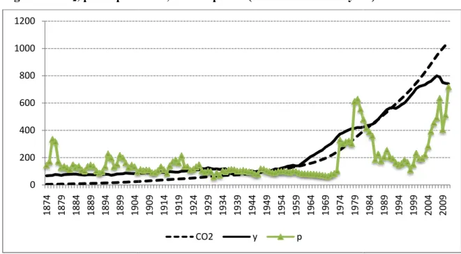
(9) 3. Sample period We focus on a sample period between 1874 and 2011 for which annual time series for CO2, GDP, population, and international oil prices are available. They are collected from different data sources. Thus, CO2 emissions measured in metric tons were obtained from the Carbon Dioxide Information Analysis Center (CDIAC) of the US Department of Energy (available at the websitehttp://cdiac.ornl.gov/). The GDP, in US dollars (1990 base year), and the population were compiled by the Maddison Historical Statistics (http://www.ggdc.net/maddison/maddison-project/home.htm) and the Instituto Nacional de Estadística (http://www.ine.es/). Finally, crude oil prices measured in real dollars (2010 base year) were gathered from the Statistical Review of World Energy 2013 provided by the British Petroleum company (http://www.bp.com/). As we can see in Figure 1, the overall evolution of CO2 emissions seems a priori a bit worrying. Indeed, the emissions in 1950 were twenty four times those generated in 1874. Whereas in 2011, they have been about two hundred and fifty times higher than those emitted at the beginning of the shown period. Regardless of the concerns caused by the emissions trend, Spain may have reached a certain level of the per capita income from which some reducing effect on emissions would have been taken place. In fact, it should be noted that the Spanish per capita income has also experienced a rather significant growth. Although in 1950 the per capita income was only about fifty percent greater than in 1874, the increase achieved in 2011 is more than eleven times that on the corresponding starting year. [Please insert Figure 1 about here] The moderate economic growth at the beginning of the sample and the extraordinary development in the past five decades respond to certain historical facts.

(10) that it is worth of briefly mentioning. In broad terms, this moderate growth sub-period in Spain came associated to a predominantly agricultural economy, with low utilization of energy resources, and scarce external relations.8 This economic growth was transitory interrupted by the Spanish Civil War (1936-1939). Under the following dictatorship government with the implementation of an autarky system, the development was somewhat conditioned by the access to limited domestic energy sources. With the aim to boost economic growth, some technocrats advocated implementing a package of deep policy reforms introduced in 1959 and following years. This change encouraged trade in general and imports of petroleum products in particular. As we can also see in Figure 1, international oil prices display some generalized growth and turbulences, which are especially relevant in the last decades. More specifically, oil prices rebounded from 1973 mainly due to the Yom Kippur War. Later on in 1978 they extraordinarily increased once more as a consequence of Iran revolution. The return to social stability in the next decade was accompanied by a falling in oil prices. They rose again but moderately this time when Iraq invaded Kuwait in 1990. After the Asian financial crisis of 1997, and mainly after Iraq’s conflict and their invasion in 2003, the oil prices greatly augmented again. Later on, the renowned Arab spring in 2010 ended a new stage of falling prices. Due to the fact that Spain is highly dependent on fuel oil imports (Sudrià, 2010), it seems quite reasonable to think that variations in international oil prices may have had. an impact on the historical evolution of Spanish CO2 emissions. Then, data on. 8. The reasonable performance of the economy in Spain during this first stage is described, for example, in Molinas and Prados de la Escosura (1989), and in Fernández Navarrete (2005)..

(11) international oil prices will be taken as a useful proxy of the (unknown) local prices for fuel oil products.. 4. Model specification and methodology. The econometric specification that explains a country’s emissions of global pollutants such as CO2 differs somewhat from those that intend to explain emissions from other pollutants. Thus, since CO2 emissions are mainly generated in industries by using oil fuel, then, an indicator of oil prices would be a reasonable variable to be introduced in the model.9 The rest of our proposed model will involve, as in the case of other pollutants, per capita real income following the standard EKC. Thus, we finally specify the next econometric model, in natural logarithms, to explain the Spanish emissions of global CO2 pollutant:. ln CO2 t = β 0 + β1 ln yt + β 2 (ln yt ) 2 + β 3 ln pt + ε t. (1). where lnyt represents per capita real income proxied by per capita GDP, and lnpt captures the evolution of real crude oil prices to which Spanish agents faced in the local market. Lastly, ε t is the error term which is assumed to be independent and normally distributed. According to the typical EKC form, we would expect that the elasticity of CO2 with respect to per capita income be positive (β1>0) and the income elasticity of its square would become negative (β2<0). Oil price elasticity for CO2 emissions would be expected to be negative (β3<0), meaning that higher prices would discourage the use of energy and therefore emissions would be lower.. 9. For the analysis of pollutants largely based on different combustion systems other energy prices should be taken into consideration. This would be the case of local pollutants such as sulfur oxide or nitrous oxide emissions, where and indicator of coal prices would be advisable to be introduced..

(12) The empirical methodology that we use in this paper is the autoregressive distributive lag (ARDL) bounds test proposed by Pesaran et al. (1997, 2001). Then, the error correction model (ECM) can be easily derived from the ARDL framework making also possible to estimate the long-run adjustment process towards equilibrium. One of the advantages of this method is that the time series regression can be carried out regardless of the nature of variables, that is, whether or not they are either I(1) or I(0). Given that most of the macroeconomic variables are proved to be either one of those two orders, then this methodology is convenient with the aim of examining long-run relationships. As Pesaran and Shin (1999) demonstrated, another great advantage is that serial correlation and endogeneity problems are removed when long-run and short-run components are simultaneously taken with appropriate lags. The relationship among per capita CO2, per capita income, and oil prices postulated in Eq. (1) follows a time path before a long-term nexus is achieved. Thus, the Eq. (1) would be written as an unrestricted error correction representation: p. p. ∆ ln CO 2t = α 0 +. ∑ i =1. α i ∆ ln CO2t −i +. ∑ i =1. p. ϕ i ∆ ln y t −i +. ∑ i =1. p. γ i ∆ (ln y t −i ) 2 +. ∑δ ∆ ln p i. i =1. t −i. +. (2). 2. + λ1 ln CO2t −1 + λ2 ln y t −1 + λ3 (ln y t −1 ) + λ4 ln pt −1 + et. where et are the new serially independent errors. The estimation procedure used here involves two stages. In a first stage we will analyze, through the ARDL bounds test, whether or not there is evidence of a cointegrating relationship. With this purpose, the null hypothesis of no cointegration among the variables ( H 0 : λ1 = λ 2 = λ3 = λ 4 = 0 ) should be tested against the alternative hypothesis ( H 1 : λ1 ≠ λ 2 ≠ λ3 ≠ λ 4 ≠ 0 ). Ordinary least squares report F-statistics, which are compared to the critical values given in Pesaran and Shin (1996), and Pesaran et al. (2001). If they go beyond the upper bound then the null hypothesis will be rejected and there will be a cointegrating relationship among the.

(13) variables. On the contrary, if the F-statistics are below the lower bound, the null hypothesis will not be rejected. In the case that the F-statistics are in between the upper and lower critical values, then the test result should be considered inconclusive. The second stage, then, is to estimate the long-run coefficients of the cointegrating relation and make inferences about their values. Finally, the empirical methodology involves the modeling of a restricted error correction representation, which takes a similar form of Eq. (2) but now including the long-run terms in the error correction variable lagged one period: p. ∆ ln CO2t = α 0 +. ∑ i =1. ∑ i =1. p. p. p. β i ∆ ln CO2t −i +. ϕ i ∆ ln y t −i +. ∑ i =1. γ i ∆ (ln y t −i ) 2 +. ∑δ ∆ ln p i. t −i. + λ ect t −1 + ε t. (3). i =1. where ectt-1 is the error correction term represented by the OLS residuals series from the long-run cointegration relationship, and the λ coefficient indicates the speed of adjustment towards this long-run equilibrium. Diagnostic and stability tests will reveal the soundness of the model.. 5. Results and discussion Since the ARDL approach does not contemplate an order higher than I(1), unit root tests will still be performed. We are aware that any structural break in the variables would reduce the power of this type of tests. If that were the case, then I(1) could not be rejected but anyhow, the aforementioned method admits both degrees I(1) and I(0) or even if it is an I(0) plus trend (TSP). The Augmented Dickey Fuller (ADF) unit root tests presented in Table 1 indicates that the four variables turned out to be of order one. [Please insert Table 1 about here].

(14) We now estimate (p+1)k number of regressions, where p is the maximum number of lags and k is the number of variables in the model, to determine the model lag selection. In order to select the optimum lag order for the model we focus on the Akaike Information Criterion (AIC) as well as the Schwarz Bayesian Criterion (BSC). We use a high enough order to ensure that the optimal one is not exceeded. As we can see in Table 2 the optimum lag order is (2, 3, 0, 2) according to the AIC, but it is (2, 2, 0, 1) according to the SBC. Based on the minimum value of the standard error of regression, we finally choose the order selected by the SBC. [Please insert Table 2 about here] When working with long time series it is advisable to pay special attention to structural changes. Thus, in order to provide stability to the model, we consider the possibility that a break or more than a break exist for intercept and trend. Since we do not know a pre-specified date for possible breaks, we will look for endogenous ones. Thus, using a trimming of 10% of the observations in each of two subsamples we check a break recursively. The one-by-one-break method based on that of Banerjee et al. (1998) keeps the analysis simple and at the same time provides easily interpretable results based on the critical values tabulated in Andrews and Ploberger (1994). For each time point, the F-statistics for testing the null hypothesis of no break is computed. Then, a break point is defined at point for which the F-statistics attains its maximum. Empirical results indicate the presence of two structural breaks, which refer to years 1917 and 1973.10 The first break coincides with World War I, which is not surprising given that Spain was benefitted from its neutrality basically through increased production in textile and metallurgical sectors. The second break point matches with the first oil shock, time when Spain enters into a deep recession given that it heavily 10. Results of including breaks one by one are available from the authors upon request..

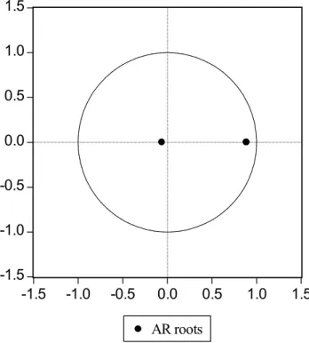
(15) depended on oil imports. The possibility of a structural change in the composition of output that might have lowered the elasticity of CO2 emissions was not found provided that the two structural breaks (1917 and 1973) of the CO2 emissions function were significant as to the intercept differentials and not to their slope ones. Next, we carry out another test to be sure that the selected model with both breaks is dynamically stable. Thus, we check that all the inverse roots of the characteristic equation associated with our ARDL model lie strictly inside the unit circle. Since this is a two-lag model (according to the selection test shown in Table 2), the number of inverse roots will also be two. The chart in form of Argand diagram in Figure 2 indicates that the two roots are real roots (they are in the X-axis) and lie inside the unit circle. Therefore, it can be confirmed that our dynamic model is stable. [Please insert Figure 2 about here] Once the properties of time series have been analyzed, the optimum lag order was determined, and different stability tests were done, we have to check whether or not a cointegrating relationship (long-run nexus) exists in the ARDL context and estimate the long run coefficients. Thus, after estimating by ordinary least squares (OLS) an Eq. (2) type (with two structural breaks in the intercept and trend), a bounds test is carried out. As we can see in Table 3, the computed F-statistics indicates that there is a cointegrating relationship among lnCO2, lny, (lny)2, and lnp at 1% level. [Please insert Table 3 about here] In order to check for the existence of an EKC we have to observe the signs of the coefficients associated to lny and (lny)2. Both coefficients have the expected signs, that is, positive for per capita income and negative for its quadratic form. The two of them.

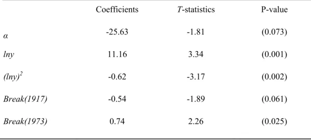
(16) are statistically significant. Now, we can obtain the estimated turning point regarding per capita income ( yˆ = exp (− λˆ. 2. / 2 λˆ3 ) ).. It is reached at 9,236 US$ (1990 base), which. approximately corresponds to per capita income in year 1980. Then, we could interpret this result by saying that from that date on, CO2 starts decreasing as per capita income grows. The specification of a cubic expression of income that would explain a likely Nshape relationship with CO2 emissions was also tested. However, the parameter associated to the cubic income variable was negative and non-significant. We also checked Dasgupta et al.‘s (2002) argument about the possibility that the environmental Kuznets curve may have begun to flatten downward under some economic changes such as technological effectiveness against pollution. The comparison of two models with technological change and without it did not help us to determine that the Spanish EKC really shifted downward during the sample period. Regarding the oil price long-run parameter, we can see that it is quite significant. Its inelasticity explains a less than proportional effect on emissions each time that there is a variation in real crude oil prices. More specifically, its magnitude is -0.39 and should be interpreted as a 1% increase in real oil prices causes a 0.39% reduction of CO2 emissions. Moreover, in order to know the importance of considering real oil price as an indicator of variations in fuel energy consumption, we have estimated a second specification model without including this variable. As we can see in Table 4, the estimated coefficients associated to lny and (lny)2 change noticeably if that indicator is excluded. In this case, the EKC would reach an earlier turning point at 8,103 US$ (1990 base), which corresponds to per capita income in year 1974. [Please insert Table 4 about here].

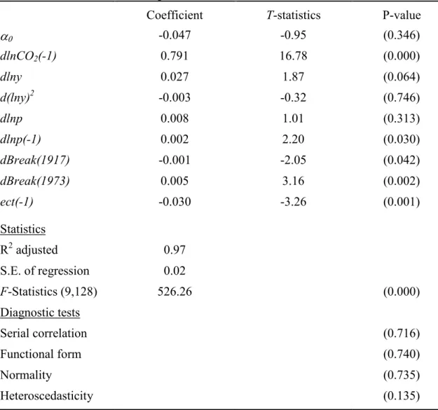
(17) Lastly, in Table 5 we can see the error correction representation for the selected model. The underlying regression passes all diagnostic tests (such as Lagrange Multiplier test for serial correlation, and heteroscedasticity, Jarque-Bera normality test of residuals, Reset test on functional form, or model specification). Furthermore, the sensitivity analysis makes the model econometrically robust. The estimated coefficients have expected signs and values. Thus, past values of CO2 (in differences) explain the evolution of CO2. The remaining short-run elasticities are (in absolute terms) lower than the long-run elasticities, which is something expected. That is, income elasticity and its quadratic form show the same signs as in the long term but now, the absolute magnitude is clearly lower. The oil price elasticity has a positive sign, but the coefficient is practically marginal and not significant. Moreover, its lagged value is significant but again close to zero. The error correction coefficient is statistically highly significant and has the correct sign (negative), which confirms the established long run relationship among the variables. This last coefficient value entails that the rate of adjustment toward the long-run equilibrium is about 3% over each year. [Please insert Table 5 about here]. 6. Conclusions The aim of this paper has been the estimation of an EKC dynamic structure for the Spanish emissions of global CO2 pollutant. The analysis carried out through the ARDL procedure considered a time period between 1874 and 2011. The fact that Spain has been traditionally highly dependent on energy consumption from fuel oil constituted a good reason not to disregard it in the EKC model specification. Failure to do so, we might have fallen into an estimation bias derived from the correlation between energy.

(18) consumption and GDP. Thus, unlike previous papers, we took into account real oil prices as a useful indicator of global pollutant energy consumption for Spain. The use of oil prices as an indicator, instead of that one related to the energy consumption, ruled out potential endogeneity problems. Even though local oil prices were unknown for the whole analyzed period, we checked the fact that Spain imported most of oil products that it consumed. Therefore, in the estimation process we included the oil prices from international markets as a reliable proxy for the variation of local oil prices. Empirical results support the idea that changes in real oil prices are relevant in order to explain the evolution of CO2 emissions. The estimated coefficients associated to per capita income and to its quadratic form have opposite signs, suggesting the presence of a turning point. This is obtained for some years later than in the case where the oil price variable was omitted. Specifically, we can infer that from 1980 the economic growth has experienced an environmental improvement through the reduction of CO2 emissions. Lastly, it is also interesting to highlight that estimated impact of real oil prices on the Spanish CO2 emissions is quite relevant from a long-run perspective. We can infer that a rise of a 1% in real oil prices causes about a 0.4% reduction of global CO2 pollutant. This outcome suggests that, in addition to the effects of per capita income, there is margin for implementing specific policy measures in order to improve the environmental quality. The knowledge about the effect of the oil price variation on the CO2 emissions provides possibilities for environmental policy decision making. Thus, the design of a new carefully energy tax structure to reduce consumption of fossil fuels and to promote other cleaner and more efficient energy resources should be seriously taken into consideration..

(19) Acknowledgements We thank two anonymous reviewers for their helpful comments. Financial support from the European Union FEDER founds and the Spanish Ministry of Economy and Competitiveness (ECO2014-58975-P) is also gratefully acknowledged.. References Agras J., Chapman D., 1999. A dynamic approach to the environmental Kuznets curve hypothesis. Ecological Economics. 28, 267-277. Andrews D.W.K., Ploberger W., 1994. Optimal tests when a nuisance parameter is present only under the alternative. Econometrica. 62, 1383-1414. Apergis, N., Ozturk, I., 2015. Testing Environmental Kuznets Curve hypothesis in Asian countries. Ecological Indicators. 52, 16-22. Bachmeier, L., Li, Q., Liu, D., 2008. Should oil prices receive so much attention? An evaluation of the predictive power of oil prices for the US economy. Economic Inquiry. 46, 528-539. Baldwin, R., 1995. Does sustainability require growth? in: Goldin, I., Winters, L.A. (Eds.), The Economics of Sustainable Development. Beacon Press, Boston, MA, pp. 19-47. Banerjee, A., Lazarova S., Urga G., 1988. Bootstrapping sequential tests for multiple structural breaks. Discussion Paper N. 17-98..

(20) Bo, S., 2011. A literature survey on environmental Kuznets curve. Energy Procedia. 5, 1322-1325. Dasgupta, S., Laplante, B., Wang, H., Wheeler, D., 2002.Confronting the environmental Kuznets curve.The Journal of Economic Perspectives. 16, 1, 147-168 Engle, R., Granger, C. 1987. Co-integration and error correction: representation, estimation, and testing. Econometrica. 55, 251-276. Esteve, V., Tamarit, C., 2012a. Is there an environmental Kuznets curve for Spain? Fresh evidence from old data. Economic Modelling. 29, 2696-2703. Esteve, V., Tamarit, C., 2012b. Threshold cointegration and nonlinear adjustment between CO2 and income: the environmental Kuznets curve in Spain, 1857–2007. Energy Economics. 34, 2148-2156. Fernández Navarrete, D., 2005. La política económica exterior del franquismo: del aislamiento a la apertura. Historia Contemporánea. 30, 49-78. Grossman, G., Krueger, A., 1991. Environmental impacts of North American free trade agreement. National Bureau of Economic Analysis. Technical report. Heil, M.T., Selden T.M., 2001. Carbon emissions and economic development: future trajectories based on historical experience. Environment and Development Economics. 6, 63-83. Kilian, L.,Vigfusson, R.J., 2013. Do oil prices help forecast us real GDP? The role of nonlinearities and asymmetries. Journal of Business and Economic Statistics. 31, 78-93..

(21) Kijima, M., Nishide, K., Ohyama, A., 2010. Economic models for the environmental Kuznets curve: A survey. Journal of Economic Dynamics and Control. 34, 11871201. Kuznets, S., 1955. Economic growth and income inequality. American Economic Review. 45, 1-28. Lardic, S., Mignon, V., 2006. The impact of oil prices on GDP in European countries: An empirical investigation based on asymmetric cointegration. Energy Policy. 34, 3910-3915. Meers, R., Leekley, R., 2000. A test of the environmental Kuznets curve for local and global pollutants. Honors projects, paper, 76. Ministerio de Industria, Energía y Turismo, 2011. Libro de la energía en España 2011. Molinas, C., Prados de la Escosura, L., 1989. Was Spain different? Spanish historical backwardness revisited. Explorations in Economic History. 26, 385-402. Panayotou, T., 1993. Empirical tests and policy analysis of environmental degradation at different stages of economic development. Working Paper WP-238, Technology and Employment Programme, ILO, Geneva. Pasten, R., Figueroa B.E., 2012. The environmental Kuznets curve: a survey of the theoretical literature. International Review of Environmental and Resource Economics. 6, 195-224. Payne, J.E., 2010. Survey of the international evidence on the causal relationship between energy consumption and growth. Journal of Economic Studies. 37, 53-95..

(22) Pesaran, M.H., Shin, Y., 1996. Cointegration and the speed of convergence to equilibrium. Journal of Econometrics. 71, 117-43. Pesaran, M.H., Pesaran, B., 1997. Working with Microfit 4.0: Interactive econometric analysis. Oxford University Press, Oxford. Pesaran, M.H., Shin, Y., 1999. An autoregressive distributed lag modelling approach to cointegration analysis, in: Strom, S. (Eds.), Econometrics and Economic Theory, in 20th Century: The Ragnar Frisch Centennial Symposium. Cambridge University Press, Cambridge. Pesaran, M.H., Shin, Y., Smith, R. J., 2001. Bounds testing approaches to the analysis of level relationships. Journal of Applied Econometrics. 16, 289-326. Richmond A.K., Kaufman R. K., 2006. Energy prices and turning points: The relationship between income and energy use/carbon emissions. Energy Journal. 7, 157-180. Roca J., Padilla E., Farre M., Galletto V., 2001. Economic growth and atmospheric pollution in Spain: Discussing the environmental Kuznets curve hypothesis. Ecological Economics. 39, 85-99. Shafik, N., Bandyopadhyay, S., 1992. Economic growth and environmental quality: time series and cross-country evidence. Background Paper for World Development Report 1992. World Bank, Washington, DC. Sephton P., Mann J., 2013. Further evidence of an environmental Kuznets curve in Spain. Energy Economics. 36, 177-181..

(23) Shahbaz, M., Hye, Q. M. A., Tiwari, A. K., Leitão, N. C., 2013. Economic growth, energy consumption, financial development, international trade and CO 2 emissions in Indonesia. Renewable and Sustainable Energy Reviews, 25, 109-121. Shahbaz, M., Lean, H. H., Shabbir, M. S., 2012. Environmental Kuznets curve hypothesis in Pakistan: cointegration and Granger causality. Renewable and Sustainable Energy Reviews, 16, 2947-2953. Shahbaz, M., Mallick, H., Mahalik, M. K., Loganathan, N., 2015. Does globalization impede environmental quality in India?. Ecological Indicators, 52, 379-393. Shahbaz, M., Sbia, R., Hamdi, H., Ozturk, I., 2014. Economic growth, electricity consumption, urbanization and environmental degradation relationship in United Arab Emirates. Ecological Indicators. 45, 622-631. Sudrià C., 1995. Energy as a limiting factor to growth, in Martín Aceña, Pablo y Simpson, James, The Economic Development of Spain since 1870, Edward Elgar, Aldershot. Tiwari, A. K., Shahbaz, M., Hye, Q. M. A., 2013. The environmental Kuznets curve and the role of coal consumption in India: Cointegration and causality analysis in an open economy. Renewable and Sustainable Energy Reviews, 18, 519-527..

(24) Figure 1. CO2, per capita pita GDP, G and oil prices (100 for 1950 basee year) year 1200 1000 800 600 400 200. 1874 1879 1884 1889 1894 1899 1904 1909 1914 1919 1924 1929 1934 1939 1944 1949 1954 1959 1964 1969 1974 1979 1984 1989 1994 1999 2004 2009. 0. CO2. y. p. The CO2 emissions series were ere obtained ob from Carbon Dioxide Information Analysis ysis C Center (CDIAC) of the US Department of Energy. The he pe per capita income (noted as y) is expressed as the ratio of o GDP to population. GDP is in real terms of 1990 US ddollars. Both variables are compiled by Maddisonn “Historical “His Statistics” and the Spanish National Institute ute of Statistics (INE). The oil prices (labeled as p) were we gathered from the Statistical Review of World Energ Energy 2013 provided by the British Petroleum..

(25) Figure 2. Inverted AR Roots from the ARDL Model 1.5 1.0 0.5 0.0 -0.5 -1.0 -1.5 -1.5. -1.0. -0.5. 0.0. 0.5. AR roots. 1.0. 1.5.

(26) Table 1. Augmented Dickey Fuller Tests ADF statistics I(1) versus I(0) lnCO2 -1.15(1). ADF statistics I(2) versus I(1) -3.12(2). ADF statistics DSP versus TSP -1.91(1). 0.70(1). -7.40(1). -1.21(1). (lny). 0.87(3). -4.95(3). -1.13(3). lnp. -2.71(1). -7.23(3). -2.93(1). -2.88. -2.88. -3.44. lny 2. Critical values. The numbers in brackets are the lags used in the ADF test in order to remove serial correlation in the residuals. DSP stands for difference stationary process and TSP means trend stationary process..

(27) Table 2. Optimum Lag Order for Model Selection AIC Order for lnCO2, lny, (lny)2, lnp (2, 3, 0, 2) Standard error of regression. 0.00219. The regressions are run based on the autoregressive distributed lag method.. SBC (2, 2, 0, 1) 0.00216.

(28) Table 3. Cointegration Results and Long Run Estimates of the ARDL Model Lower bounds Upper bounds F-statistics 10% 5% 1% 10% 5% 1% 2.45 2.86 3.74 3.52 4.01 5.06 F(4,122)= 6.3399 Coefficients. T-statistics. P-value. -10.31. -0.77. (0.444). lny. 7.67. 2.53. (0.012). (lny)2. -0.42. -2.40. (0.018). lnp. -0.39. -2.24. (0.027). Breack(1917). -0.48. -2.27. (0.025). Breack(1973). 0.65. 2.61. (0.010). α. Sensitivity analysis and other statistics are provided in the error correction model..

(29) Table 4. Long Run Estimates of the ARDL Model Without Oil Prices Coefficients. T-statistics. P-value. α. -25.63. -1.81. (0.073). lny. 11.16. 3.34. (0.001). (lny)2. -0.62. -3.17. (0.002). Break(1917). -0.54. -1.89. (0.061). Break(1973). 0.74. 2.26. (0.025).

(30) Table 5. Error Correction Representation for the Selected Model Coefficient. T-statistics. P-value. α0. -0.047. -0.95. (0.346). dlnCO2(-1). 0.791. 16.78. (0.000). dlny. 0.027. 1.87. (0.064). d(lny). -0.003. -0.32. (0.746). dlnp. 0.008. 1.01. (0.313). dlnp(-1). 0.002. 2.20. (0.030). dBreak(1917). -0.001. -2.05. (0.042). dBreak(1973). 0.005. 3.16. (0.002). ect(-1). -0.030. -3.26. (0.001). 2. Statistics R2 adjusted. 0.97. S.E. of regression. 0.02. F-Statistics (9,128). 526.26. (0.000). Diagnostic tests Serial correlation. (0.716). Functional form. (0.740). Normality. (0.735). Heteroscedasticity. (0.135). Variables starting with a d means differenced once; variables lagged one period are expressed as (-1); ect is the error correction term..

(31)