TítuloHighway travel time information system based on cumulative count curves and new tracking technologies

Texto completo

(1)CIT2016 – XII Congreso de Ingeniería del Transporte València, Universitat Politècnica de València, 2016. DOI: http://dx.doi.org/10.4995/CIT2016.2016.3209 .. 1336. Highway travel time information system based on cumulative count curves and new tracking technologies Francesc Soriguera Martí Associate Professor, CENIT - UPC-BarcelonaTech, Spain Margarita Martínez-Díaz Assistant Professor, Universidade da Coruña, Spain Ignacio Pérez Pérez Associate Professor, Universidade da Coruña, Spain. ABSTRACT Travel time is probably the most important indicator of highway level of service, and it is also the most appreciated information for highway users. Administrations and private companies make increasing efforts to improve its real time estimation. The appearance of new technologies makes the precise measurement of travel times easier than never before. However, direct measurements of travel time are, by nature, outdated for real time applications, and lack of the desired forecasting capabilities. This paper introduces a new methodology to improve the real time estimation of travel times by using the equipment usually present in most highways, i.e., loop detectors, in combination with the newer Automatic Vehicle Identification or Tracking Technologies. One of the most important features of the method is the usage of cumulative counts at detectors as an input, avoiding the drawbacks of common spot-speed methodologies. Cumulative count curves have great potential for freeway travel time information systems, as they provide spatial measurements, allowing the calculation of instantaneous travel times. In addition, vehicle accumulation exhibits predictive capabilities. Nevertheless, they have not been extensively used mainly because of the error introduced by the accumulation of the detector drift. The proposed methodology solves this problem by correcting the deviations using direct travel time measurements. The method results highly beneficial for its accuracy as well as for its low implementation cost. 1. INTRODUCTION Travel time is undoubtedly a valuable information both for drivers and traffic management centers. Modern technologies have brought a renewed interest in the improvement of current estimation procedures. Nowadays, several techniques allow the direct measurement of travel time, either based on Automated Vehicle Identification (AVI) or on tracking technologies. License plates (using video recognition) or the Bluetooth signature of on-board devices are used to identify vehicles, while GPS is usually used for tracking. These methods supply accurate measurements of vehicles' travel time. However, they lack predictive capabilities,. This work is licensed under a Creative Commons Attribution-NonCommercial-NoDerivatives 4.0 International License (CC BY-NC-ND 4.0)..

(2) 1337. CIT2016 – XII Congreso de Ingeniería del Transporte València, Universitat Politècnica de València, 2016. DOI: http://dx.doi.org/10.4995/CIT2016.2016.3209 .. meaning that the measurement is obtained when the trip has ended, and provides very little information on its future evolution. Thus, their applicability in real time information systems is limited. Indirect travel time estimation from fundamental traffic variables appears as an alternative. Traditionally, spot-speed methods based on loop detectors data have been used. Nevertheless, several research studies point out their inaccuracy in case of congestion or with low detector density (Soriguera and Robusté, 2010; Martínez-Díaz and Pérez, 2015) and they do not help in predicting travel times either. Methods based on cumulative count curves have not seen great success. Mainly, this is due to the systematic detector drift phenomenon. The count drift between input and output detectors is accumulated in these methods, leading to large errors in the results (Coifman and Cassidy, 2002; Nam and Drew, 1996; Oh et al., 2003). However, input-output methods have two important advantages: first, there is no need for a big density of detectors; and second and most importantly, these methods exhibit forecasting capabilities because the accumulation of vehicles to be served in the near future is known (Soriguera and Robusté, 2010). The main goal of this paper is the introduction of a new methodology for travel time estimation in real time that takes advantage of the predictive ability of cumulative count methods and that uses direct measurements of travel time to correct the detector drift. The method is especially suited for being applied in congested conditions, when travel time information is more relevant and when all other methods are less accurate. Its implementation turns to be easy and cheap. The paper is organized as follows: Section 2 contains an overview of the methodology. Section 3 presents the test site and the data that are being used for the implementation of the algorithm. Finally, in Section 4, the current state of development of the research and some additional issues planned for a near future are explained. 2. METHODOLOGY 2.1 Input – output diagrams revisited Figure 1 shows a typical cumulative count input - output diagram. (A) is the "arrivals" count curve measured at the upstream detector (xu) and accumulated in time. (D) is the "departures" cumulative count curve measured at the downstream detector (xd). (V) is a "virtual" curve, representing the departures curve that would have been measured in the absence of delay. (V) is obtained by simply shifting forward in time the (A) curve a magnitude equal to the free flow travel time. In case the free flow travel time is significantly smaller than the loop detector aggregation period (Δt), the construction of (V) is simpler, as the free flow travel. This work is licensed under a Creative Commons Attribution-NonCommercial-NoDerivatives 4.0 International License (CC BY-NC-ND 4.0)..

(3) CIT2016 – XII Congreso de Ingeniería del Transporte València, Universitat Politècnica de València, 2016. DOI: http://dx.doi.org/10.4995/CIT2016.2016.3209 .. 1338. time and the initial accumulation m(0) can be neglected. Sections between loops of 2 Km or less, increasingly common in freeways, ensure this condition. See Daganzo (1997) for a review on these concepts and their application. Working with the (V) and (D) curves allows easily obtaining delays while eliminating the need for keeping track of the accumulation. By definition, the excess accumulation is zero until congestion appears. Or equivalently, (V) and (D) curves coincide while free-flow prevails. This by itself limits to a large extend the problems of the detector drift (Soriguera, 2016). Figure 5 assumes FIFO traffic (First in - First out, i.e. no significant passing). Freeway traffic can be considered a FIFO system in congested conditions, when multilane behavior is very limited and its effects on travel times are negligible (Muñoz and Daganzo, 2002). In addition, because the interest is not in individual vehicle travel times, but on the average, one can assume that vehicle switch labels when passing, so that FIFO holds (Daganzo, 1997). N. A(Xu_i,t) V(Xd_i,t) 𝑎𝑐𝑐𝑢𝑚𝑢𝑙𝑎𝑡𝑖𝑜𝑛. D(Xd_i,t). 𝑡𝑟𝑎𝑣𝑒𝑙 𝑡𝑖𝑚𝑒 𝑒𝑥𝑐𝑒𝑠𝑠 𝑎𝑐𝑐𝑢𝑚𝑢𝑙𝑎𝑡𝑖𝑜𝑛 free flow 𝑡𝑟𝑎𝑣𝑒𝑙 time. 𝑑𝑒𝑙𝑎𝑦. m(0). Fig. 1 – Graphical interpretation of cumulative curves. t. The algorithm turns on when congestion is detected. This happens on a section either if the speed at the upstream or downstream detector is lower than the free flow speed or if the slope of the virtual arrivals curve is bigger than that of the departures curve. All these comparisons take into account statistical variations. The algorithm turns off as soon as both curves, (V) and (D) coincide at some point in time. 2.2 Drift correction from direct travel time measurements Figure 2 shows the simplest situation that the methodology will face. This is a freeway stretch defined by the upstream (Xus) and downstream (Xds) positions of the direct measurement devices. The stretch contains several sections defined by the location of loop detectors. In case that the direct measurements are obtained using tracking technologies. This work is licensed under a Creative Commons Attribution-NonCommercial-NoDerivatives 4.0 International License (CC BY-NC-ND 4.0)..

(4) CIT2016 – XII Congreso de Ingeniería del Transporte València, Universitat Politècnica de València, 2016. DOI: http://dx.doi.org/10.4995/CIT2016.2016.3209 .. 1339. every stretch would correspond to a single section. Because the methodology is based on vehicle conservation, a closed measurement system is required. This means that, although the number of detectors does not need to be large, on/off ramps need to be monitored, in addition to the main trunk.. Fig. 2 – Typical detection configuration on a simple freeway stretch The updating time interval of loop detectors (Δt) is generally shorter than that of the direct measurement devices (ΔT), as direct measurements need a significant amount of time to obtain a sample big enough to compute reliable averages. This means that, in addition to the spatial alignment of measurements, temporal alignment will also be necessary. ̂𝑠 (𝑡)). This Direct measurements provide the average travel time on the stretch at time t (𝑡𝑡 ̂𝑠 (𝑡)), as in can be expressed as the sum of the free flow travel time (𝑡𝑓𝑠 ) plus the delay (𝑤 Equation 1: ̂𝑠 (𝑡) = 𝑡𝑓𝑠 + 𝑤 ̂𝑠 (𝑡) 𝑡𝑡. (1). Delay on the stretch (𝑤 ̂ 𝑠 (𝑡)), is the sum of the delays encountered by the drivers on the component sections (𝑤 ̂𝑖 (𝑡 ′ )) (see Equation 2). (𝑡 ′ ) stands for the fact that the reference time is trajectory based, and therefore temporal alignment is necessary. 𝑤 ̂ 𝑠 (𝑡) = ∑𝑛𝑖=1 𝑤 ̂𝑖 (𝑡 ′ ). (2). Component delays (𝑤 ̂𝑖 (𝑡 ′ )) on each section are not available from direct measurements. However, loops can provide this information. From every pair of input-output curves the current average delay on each section (𝑤𝑖 (𝑡 ′ )) can be obtained, although affected by the cumulative curve drift errors. Despite the long term drift of each pair of detectors (Section (i)) is addressed by multiplying the raw counts by a correction factor (β) (see Equations 3 and 4), this is not enough to provide accurate real time information, as short-term drift is also significant and not systematic. ∑24ℎ 𝑛𝑑_𝑖,𝑡. 𝑡=0 𝛽𝑖 = ∑24ℎ. 𝑡=0 𝑛𝑢_𝑖,𝑡. (3). This work is licensed under a Creative Commons Attribution-NonCommercial-NoDerivatives 4.0 International License (CC BY-NC-ND 4.0)..

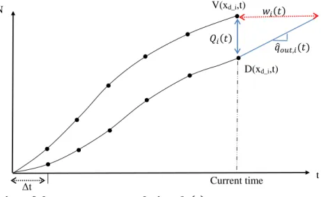
(5) CIT2016 – XII Congreso de Ingeniería del Transporte València, Universitat Politècnica de València, 2016. DOI: http://dx.doi.org/10.4995/CIT2016.2016.3209 .. 1340. 𝑛𝑒𝑤 𝑛𝑢_𝑖,𝑡 = 𝛽𝑖 · 𝑛𝑢_𝑖,𝑡. (4). Where (𝑛𝑢_𝑖,𝑡 ) and (𝑛𝑑_𝑖,𝑡 ) are the traffic counts at the upstream and downstream detectors of Section (i) at time interval (t). From now on, the long-term drift will be assumed to be corrected, although not explicitly stated in the equations. The aim of the methodology is to correct the short term drift errors in cumulative count curves by using direct measurements. To that end it is necessary to divide the total directly measured delay (𝑤 ̂ 𝑠 (𝑡)) among the component sections (𝑤 ̂𝑖 (𝑡 ′ )). It is assumed that the proportion of the delay in a particular section with respect to the total of the stretch is the same despite working with direct or indirect measurements (see Equation 5). This assumption is acceptable even though the indirect values have not been corrected yet. 𝑤𝑖 (𝑡 ′ ). 𝑤 ̂𝑖 (𝑡 ′ ) = ∑𝑛. 𝑖=1 𝑤𝑖 (𝑡. ′). ∙𝑤 ̂ 𝑠 (𝑡). (5). If there were no drift, (𝑤 ̂𝑖 (𝑡 ′ )) estimated from direct measurement, and 𝑤𝑖 (𝑡 ′ ) measured from input-output curves, would be equal. This property allows computing a short term drift correction factor (𝛼𝑖 ) (Equation 6 and 7): 𝑛𝑒𝑤 𝑛𝑢_𝑖,𝑡 = 𝛼𝑖 · 𝛽𝑖 · 𝑛𝑢_𝑖,𝑡. (6). 𝛼𝑖 obtained so that 𝑤 ̂𝑖 (𝑡 ′ ) = 𝑤𝑖 (𝑡 ′ ). (7). Care must be taken when computing the average delay (𝑤𝑖 (𝑡 ′ )) from input-output curves Different estimation processes must be applied depending on the nature of the direct measurements for the comparison. For example, AVI technologies deliver arrival-based travel times (i.e. they are only known once the vehicle has finished its route in the link). Accordingly, (𝑤𝑖 (𝑡 ′ )) needs to represent an arrival based travel time. Therefore, (𝑤𝑖 (𝑡 ′ )) should be computed as the area enclosed between (V) and (D) curves and only for the vehicles crossing the downstream detector (xd) during the time interval (t), divided by this number of vehicles. In contrast, tracking technologies supply instantaneous travel times. Then, (𝑤𝑖 (𝑡 ′ )) should be computed as the area enclosed between (V) and (D) curves between times (t–Δt) and (t) and divided by the number of vehicles crossing the downstream detector during the time interval. These different travel time definitions are overlooked in previous studies (Nam and Drew, 1996; Oh et al., 2003, van Arem et al., 1997). 𝑛𝑒𝑤 With the corrected (V) curve (i.e. constructed from (𝑛𝑢_𝑖,𝑡 ), it is possible to calculate the current accumulation 𝑄𝑖 (𝑡) as the difference between the current values of (V) and (D) curves. 𝑄𝑖 (𝑡) is the key spatial value that allows computing predicted travel times, as Equation 8 and Figure 3 show:. This work is licensed under a Creative Commons Attribution-NonCommercial-NoDerivatives 4.0 International License (CC BY-NC-ND 4.0)..

(6) CIT2016 – XII Congreso de Ingeniería del Transporte València, Universitat Politècnica de València, 2016. DOI: http://dx.doi.org/10.4995/CIT2016.2016.3209 .. 1341. 𝑤𝑖 (𝑡) =. 𝑄𝑖 (𝑡). (8). 𝑞̂𝑜𝑢𝑡,𝑖 (𝑡). Where 𝑤𝑖 (𝑡) is the predicted delay in Section (i) and (𝑞̂𝑜𝑢𝑡,𝑖 (𝑡)) is the last statistical significant estimation of the average outflow at downstream detector. Finally, the predicted travel time on the stretch (𝑡𝑡 𝑠 (𝑡)) is obtained by adding up all predicted section delays (𝑤 𝑠 (𝑡)) plus the free flow travel time. V(xd_i,t). N. 𝑤𝑖 (𝑡). 𝑄𝑖 (𝑡). 𝑞̂𝑜𝑢𝑡,𝑖 (𝑡) D(xd_i,t). Δt. Current time. t. Fig. 3 – Estimation of the current accumulation 𝑸𝒊 (𝒕) 2.3 Merging and diverging flows (V) and (D) curves must account for mergings and divergings when they exist. The issue here is that count measurements at on/off ramps need to be “shifted” to the location of upstream or downstream detectors. Newell (1993) proposes a methodology to shift cumulative count curves consistent with LWR theory of traffic flow (Lighthill and Whitham, 1955; Richards, 1956). However, the method requires the capacity of the section as an input. For real time applications, because capacity changes and depends on the particular incidents for a given day, the method results overcomplicated. A simpler solution is proposed here. The net flows at the junction (i.e. the difference between inflows and outflows with the appropriate sign) are transferred to the nearest trunk detector. This procedure assumes that through vehicles experience the same delay than those entering or exiting the section by the junction. Although this might not be true in some contexts, the over or underestimations of individual travel times do not imply a big error in the average final results, as long as the number of through vehicles is big in comparison to the rest. 3. IMPLEMENTATION Preliminary results achieved to date are promising. A pilot test is being carried out on the AP-7 highway, which runs along the Spanish Mediterranean cost. Specifically, the available. This work is licensed under a Creative Commons Attribution-NonCommercial-NoDerivatives 4.0 International License (CC BY-NC-ND 4.0)..

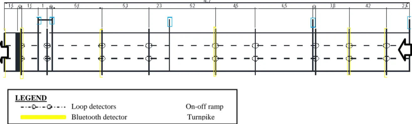
(7) CIT2016 – XII Congreso de Ingeniería del Transporte València, Universitat Politècnica de València, 2016. DOI: http://dx.doi.org/10.4995/CIT2016.2016.3209 .. 1342. data belong to its northeast part, with a length of 45.7 Km, from the Maçanet-Blanes junction to the turnpike at La Roca del Vallès, near Barcelona. Available data include traffic counts and spot speeds from double loop detectors (Δt = 3 min), Bluetooth vehicle identifications (ID and time stamp and average, ΔT = 6 min), and the entrance / exit times of every vehicle from toll tickets. Five different stretches are defined by the position of the Bluetooth detectors (see Figure 4). Each one has different characteristics: number of loop detectors (i.e. sections) within the stretch, number of lanes, and existence of junctions (or not). This diversity will add robustness to the final results.. LEGEND Loop detectors Bluetooth detector. On-off ramp Turnpike. Fig. 4 - Test site layout 4. ONGOING WORK AND FUTURE RESEARCH The methodology is currently being tested under different boundary conditions. The results achieved so far match the expectations. Nevertheless, its robustness and its exact degree of accuracy still need to be proved. Ongoing research will allow drawing quantitative conclusions. Additionally, some future research lines have been already outlined. For example, the sensitivity of the method on factors such as the detector density, the geometry of the freeway (e.g. number of lanes or junctions) or the frequency of overtaking will be investigated. Further research will also include the integration of the method together with the most relevant tools for real time traffic management, in order to assess their potential improvement.. 5. REFERENCES. This work is licensed under a Creative Commons Attribution-NonCommercial-NoDerivatives 4.0 International License (CC BY-NC-ND 4.0)..

(8) 1343. CIT2016 – XII Congreso de Ingeniería del Transporte València, Universitat Politècnica de València, 2016. DOI: http://dx.doi.org/10.4995/CIT2016.2016.3209 .. COIFMAN, B., and CASSIDY, M. (2002). Vehicle reidentification and travel time measurement on congested freeways. Transportation Research Part A 36(10), pp. 899917. DAGANZO, C. (1997). Fundamentals of Transportation and Traffic Operations. Pergamon, Oxford. ISBN: 0080427855. LIGHTHILL M.J. and G.B. WHITHAM, G.B. (1955). On kinematic waves-II. A theory of traffic flow on long crowded roads. Proceedings of the Royal Society of London. Series A, Mathematical and Physical Sciences 229(1178), pp. 317-345. MARTÍNEZ-DÍAZ, M. and PÉREZ, I. (2015). A simple algorithm for the estimation of road traffic space mean speeds from data available to most management centres. Transportation Research Part B 75, pp. 19-35. MUÑOZ, J. C. and DAGANZO. C.F. (2002). The bottleneck mechanism of a freeway diverge. Transportation Research Part A 36(6), pp. 483-505. NAM, D.H. and DREW, D.R. (1996). Traffic dynamics: Method for estimating freeway travel times in real time from flow measurements. ASCE Journal of Transportation Engineering 122(3), pp. 185-191. NEWELL, G. F. (1993). A simplified theory of kinematic waves in highway traffic. Part I: General Theory; Part II: Queuing at freeway bottlenecks. Part III: Multi-destination flows. Transportation Research Part B 27(4), 281-313. OH, J.S.; JAYAKRISHNAN, R. and RECKER, W. (2003). Section travel time information from point detection data. Proceedings of the 82nd Transportation Research Board Annual Meeting. Washington D.C. RICHARDS, P.I. (1956). Shockwaves on the highway. Oper. Res. 4, pp. 42-51. SORIGUERA, F. and ROBUSTÉ, F. (2010). Highway travel time accurate measurement and short-term prediction using multiple data sources. Transportmetrica 7(1), pp. 85-109. SORIGUERA, F. and ROBUSTÉ, F. (2013). Freeway travel-time information: design and real time performance using spot-speed methods. IEEE Transactions on Intelligent Transportation Systems 14(2), pp. 731-742. SORIGUERA, F. (2016). Highway travel time estimation with data fusion. Springer, Berlín. ISBN: 978-3-662-48856-0. VAN AREM, E.; VAN DER VLIST, M.J.M.; MUSTE, R.M. and SMULDERS, S.A. (1997). Travel Time estimation in the GERIDIEN project. International Journal of Forecasting 13, pp. 73-85.. This work is licensed under a Creative Commons Attribution-NonCommercial-NoDerivatives 4.0 International License (CC BY-NC-ND 4.0)..

(9)