Identification of optimal strategies in tennis using broadcast video sequences and machine learning
131
0
0
Texto completo
(2) 2.
(3) A mi mujer Maria y mis tres hijos, Carla, Nina y Jamie.. i.
(4) ii.
(5) Acknowledgements I would like to thank my supervisors Dr. Javier Varona and Dra. Margarita Miró, for their guidance throughout the course of this work, which has been especially challenging at times due to its long-distance nature. I would also like to thank Dr. Walter Kosters for his help on the data mining articles and for the always stimulating technical discussions on this work. Special thanks also go to Dr. Bill Christmas for supporting me at the initial stages of this thesis and letting me use their computer vision framework and libraries. I would also like to thank Dr. Jean-Bernard Hayet for his support during the implementation of the Fast-Projection algorithm and for being so accessible when needed. Many thanks also go to Dr. David Sanz who has reviewed all the tennis-specific aspects of this thesis and has introduced me to several professional tennis coaches who were able to provide invaluable input into this work. Finally, and most importantly, I would like to express my deepest gratitude to my wife Maria for the love and support she has shown to me during this long, and sometimes complicated journey.. iii.
(6) iv.
(7) Abstract The analysis of tennis sequences from broadcast videos has been studied before with an aim to automatically annotate the score or to classify the content for later retrieval, but seldom with a tactical aim. This work focuses therefore in designing a system able to perform tactical analysis in tennis games. The main objectives of such a system include the identification of the most frequent patterns displayed by a player in a game, and the discovery of optimal sequences of strokes that maximize the probability for a player to beat the opponent. The proposed system must also be able to translate the results into a high-level and user-friendly language. To do so, it is fundamental to start off with an accurate notational representation of a tennis game. This representation must incorporate the majority of variables that intervene in the game, such as the players positions, the ball bouncing positions, the strokes performed, the ball effects, the distances run, the score, etc. In order to obtain this information, a semi-automatic system is proposed and implemented. Once this accurate data has been gathered, and with a view to achieve the objectives aforementioned, this thesis explores this information from two different angles. A first one, based on multivariate sequential data mining, in an attempt to discover game patterns and player characterization; and a second one, based on reinforcement learning and artificial intelligence with an aim to identify optimal potential sequences of strokes that would improve the chances of winning. In this way, the system is able to suggest the most appropriate strategy for each of the players. To showcase the tactical conclusions and the overall process, this work analyzes several real tennis matches and displays graphically the results obtained. Key words: Sports Broadcast Video Analysis; Tennis; Markov Decision Processes; Monte Carlo Simulations; Optimal Policies; Sequential Data Mining. v.
(8) vi.
(9) Resumen La anotación automática de secuencias de videos deportivos partiendo de retransmisiones televisivas ha sido estudiada con anterioridad con el fin de conseguir sistemas capaces de detectar y clasificar las secuencias, pero pocas veces con una finalidad táctica. Este trabajo se centra por tanto en conseguir un sistema capaz de realizar análisis tácticos de partidos de tenis. Los objetivos de dicho sistema incluyen la identificación de las secuencias de golpes más utilizadas por los jugadores, ası́ como el descubrimiento de las secuencias óptimas de golpes que maximicen las probabilidades de un jugador de ganar a su contrincante. Por último, el sistema debe ser capaz de trasladar estos resultados a un lenguaje sencillo y fácilmente visualizable. Para ello, y como condición sine qua non, es preciso partir de una representación notacional muy aproximada y completa de un partido de tenis. Una representación que incorpore con exactitud la mayorı́a de las variables que intervienen en el desarrollo del juego (posiciones de los jugadores, posición del bote de la pelota, golpe efectuado, efectos sobre la pelota, distancias recorridas, marcador, etc.). Para conseguir esto, ha sido necesario en primer lugar desarrollar un sistema semi-automatico de visión por ordenador que capture la información relevante. Una vez obtenida dicha representación, y para poder conseguir los objetivos señalados anteriormente, esta tesis explora dichos datos desde dos perspectivas distintas. Una primera, basada en la minerı́a de datos secuencial, cuyo objetivo es el descubrimiento de patrones de juego y la caracterización de los jugadores. Y una segunda, basada en el aprendizaje por refuerzo y en la inteligencia artificial, centrada en identificar potenciales secuencias óptimas de golpes. De esta forma, el sistema es capaz de sugerir la estrategia más apropiada para cada uno de los jugadores. Para comprobar las conclusiones tácticas, ası́ como el procedimiento seguido, este trabajo analiza varios partidos reales de tenis y muestra gráficamente los resultados obtenidos. vii.
(10) viii Palabras Claves: Procesado de Videos Deportivos; Tenis; Procesos de Decisión de Markov; Simulaciones de Monte Carlo; Polı́ticas Óptimas; Minerı́a de Datos Secuencial..
(11) Contents 1 Introduction. 1. 1.1. Related Work . . . . . . . . . . . . . . . . . . . . . . . . . . . . . . . . . . .. 3. 1.2. Motivation. . . . . . . . . . . . . . . . . . . . . . . . . . . . . . . . . . . . .. 5. 1.3. Scientific Contribution . . . . . . . . . . . . . . . . . . . . . . . . . . . . . .. 5. 1.4. Overview of this Thesis . . . . . . . . . . . . . . . . . . . . . . . . . . . . .. 6. 1.5. Overview of Publications . . . . . . . . . . . . . . . . . . . . . . . . . . . . .. 7. 2 Annotation System 2.1. 2.2. 2.3. 9. System Description . . . . . . . . . . . . . . . . . . . . . . . . . . . . . . . .. 10. 2.1.1. Introduction . . . . . . . . . . . . . . . . . . . . . . . . . . . . . . .. 10. 2.1.2. System Design . . . . . . . . . . . . . . . . . . . . . . . . . . . . . .. 10. 2.1.3. High Level Overview . . . . . . . . . . . . . . . . . . . . . . . . . . .. 15. Pre-Processing . . . . . . . . . . . . . . . . . . . . . . . . . . . . . . . . . .. 15. 2.2.1. Luminance Filter . . . . . . . . . . . . . . . . . . . . . . . . . . . . .. 17. 2.2.2. Texture Filter . . . . . . . . . . . . . . . . . . . . . . . . . . . . . . .. 19. 2.2.3. Linearity Filter . . . . . . . . . . . . . . . . . . . . . . . . . . . . . .. 20. 2.2.4. Probabilistic Hough Filter . . . . . . . . . . . . . . . . . . . . . . . .. 21. 2.2.5. Selection of the Main Lines . . . . . . . . . . . . . . . . . . . . . . .. 22. Automatic Calibration of Broadcast Images . . . . . . . . . . . . . . . . . .. 25. 2.3.1. Previous Work . . . . . . . . . . . . . . . . . . . . . . . . . . . . . .. 25. 2.3.2. Homography . . . . . . . . . . . . . . . . . . . . . . . . . . . . . . .. 26. 2.3.3. Fast Projection Algorithm . . . . . . . . . . . . . . . . . . . . . . . .. 28. 2.3.4. Hypothesis Generation . . . . . . . . . . . . . . . . . . . . . . . . . .. 32. 2.3.5. Hypothesis Evaluation . . . . . . . . . . . . . . . . . . . . . . . . . .. 33. 2.3.6. Homography Matrix Calculation . . . . . . . . . . . . . . . . . . . .. 35. ix.
(12) x. CONTENTS 2.3.7. Results . . . . . . . . . . . . . . . . . . . . . . . . . . . . . . . . . .. 36. 2.4. Court Tracking . . . . . . . . . . . . . . . . . . . . . . . . . . . . . . . . . .. 37. 2.5. Conclusions . . . . . . . . . . . . . . . . . . . . . . . . . . . . . . . . . . . .. 42. 3 Data Mining and Pattern Discovery 3.1. 45. Formalization . . . . . . . . . . . . . . . . . . . . . . . . . . . . . . . . . . .. 46. 3.1.1. Definitions . . . . . . . . . . . . . . . . . . . . . . . . . . . . . . . .. 47. 3.1.2. Reference Model . . . . . . . . . . . . . . . . . . . . . . . . . . . . .. 48. 3.1.3. Attributes Considered . . . . . . . . . . . . . . . . . . . . . . . . . .. 49. Multi-variate similarity-based sequential pattern mining . . . . . . . . . . .. 50. 3.2.1. Similarity measure . . . . . . . . . . . . . . . . . . . . . . . . . . . .. 50. 3.2.2. Visualization . . . . . . . . . . . . . . . . . . . . . . . . . . . . . . .. 52. 3.2.3. Similarity thresholds . . . . . . . . . . . . . . . . . . . . . . . . . . .. 52. 3.2.4. Mining Problems . . . . . . . . . . . . . . . . . . . . . . . . . . . . .. 54. Mining Problem 1 . . . . . . . . . . . . . . . . . . . . . . . . . . . . . . . .. 55. 3.3.1. Sequential Pattern Mining . . . . . . . . . . . . . . . . . . . . . . . .. 55. 3.3.2. Clustering . . . . . . . . . . . . . . . . . . . . . . . . . . . . . . . . .. 58. 3.3.3. Weighted centroids . . . . . . . . . . . . . . . . . . . . . . . . . . . .. 60. Mining Problem 2 . . . . . . . . . . . . . . . . . . . . . . . . . . . . . . . .. 61. 3.4.1. Identification of unbalancing events . . . . . . . . . . . . . . . . . . .. 61. 3.4.2. Winning patterns . . . . . . . . . . . . . . . . . . . . . . . . . . . . .. 62. 3.4.3. Completion of attack patterns . . . . . . . . . . . . . . . . . . . . . .. 63. 3.4.4. Pattern prequel and sequel . . . . . . . . . . . . . . . . . . . . . . .. 64. 3.5. Mining Problem 3 . . . . . . . . . . . . . . . . . . . . . . . . . . . . . . . .. 67. 3.6. Results . . . . . . . . . . . . . . . . . . . . . . . . . . . . . . . . . . . . . . .. 68. 3.6.1. Mining Problems 1 and 2 . . . . . . . . . . . . . . . . . . . . . . . .. 68. 3.6.2. Mining Problem 3 . . . . . . . . . . . . . . . . . . . . . . . . . . . .. 71. Conclusions . . . . . . . . . . . . . . . . . . . . . . . . . . . . . . . . . . . .. 72. 3.2. 3.3. 3.4. 3.7. 4 Identification of optimal strategies. 73. 4.1. Change of paradigm . . . . . . . . . . . . . . . . . . . . . . . . . . . . . . .. 74. 4.2. Tennis as a Markov Process . . . . . . . . . . . . . . . . . . . . . . . . . . .. 75. 4.2.1. Initial Model . . . . . . . . . . . . . . . . . . . . . . . . . . . . . . .. 76. 4.2.2. Full Tennis Model . . . . . . . . . . . . . . . . . . . . . . . . . . . .. 81.
(13) CONTENTS 4.3. 4.4. 4.5. xi. Monte Carlo Tree Search (MCTS) . . . . . . . . . . . . . . . . . . . . . . .. 86. 4.3.1. Algorithm structure . . . . . . . . . . . . . . . . . . . . . . . . . . .. 87. 4.3.2. Simulation . . . . . . . . . . . . . . . . . . . . . . . . . . . . . . . .. 88. 4.3.3. Back-propagation . . . . . . . . . . . . . . . . . . . . . . . . . . . . .. 88. 4.3.4. Selection. . . . . . . . . . . . . . . . . . . . . . . . . . . . . . . . . .. 90. 4.3.5. Expansion . . . . . . . . . . . . . . . . . . . . . . . . . . . . . . . . .. 90. 4.3.6. Algorithm . . . . . . . . . . . . . . . . . . . . . . . . . . . . . . . . .. 90. Experiments . . . . . . . . . . . . . . . . . . . . . . . . . . . . . . . . . . . .. 91. 4.4.1. Initial Model . . . . . . . . . . . . . . . . . . . . . . . . . . . . . . .. 91. 4.4.2. Full Tennis Model . . . . . . . . . . . . . . . . . . . . . . . . . . . .. 93. Conclusions and further research . . . . . . . . . . . . . . . . . . . . . . . .. 98. 5 Conclusions. 101. Bibliography . . . . . . . . . . . . . . . . . . . . . . . . . . . . . . . . . . . . . . 103.
(14) xii. CONTENTS.
(15) List of Figures 1.1. Screenshot of Dartfish software . . . . . . . . . . . . . . . . . . . . . . . . .. 2. 2.1. Data Capture and Annotation System . . . . . . . . . . . . . . . . . . . . .. 11. 2.2. Ball position in broadcast image and in reference court . . . . . . . . . . . .. 12. 2.3. Annotation system overview . . . . . . . . . . . . . . . . . . . . . . . . . . .. 15. 2.4. High level flowchart for the homography calculation and tracking . . . . . .. 16. 2.5. Histograms of the images’ central area for a clay court (left) and a one-color hard court (right) . . . . . . . . . . . . . . . . . . . . . . . . . . . . . . . . .. 2.6. 18. Histograms of the images’ central area for a two-color hard court (left) and a grass court (right) . . . . . . . . . . . . . . . . . . . . . . . . . . . . . . .. 18. 2.7. Luminance threshold calculation . . . . . . . . . . . . . . . . . . . . . . . .. 18. 2.8. Image after applying luminance filter (left) and the result after applying a texture filter with sp = 7 × 7 (right) . . . . . . . . . . . . . . . . . . . . . .. 2.9. 20. Image after applying a texture filter with sp = 3 × 3 (left) and image after applying the Canny filter (right) . . . . . . . . . . . . . . . . . . . . . . . .. 20. 2.10 Image after applying the linearity filter. τ = 1 (left) τ = 3 (center) and τ = 5 (right) . . . . . . . . . . . . . . . . . . . . . . . . . . . . . . . . . . .. 21. 2.11 Lines detected by the probabilistic Hough transform . . . . . . . . . . . . .. 22. 2.12 Detected segments along the lines . . . . . . . . . . . . . . . . . . . . . . . .. 23. 2.13 Main line selection after applying different methods . . . . . . . . . . . . . .. 25. 2.14 Transformation between the image plane and the reference plane . . . . . .. 27. 2.15 Vanishing points for a typical broadcast perspective . . . . . . . . . . . . .. 28. 2.16 Cross Ratio definition . . . . . . . . . . . . . . . . . . . . . . . . . . . . . .. 29. 2.17 Terminology used in fast projection . . . . . . . . . . . . . . . . . . . . . . .. 30. 2.18 Line (p, pv ) on the projected image . . . . . . . . . . . . . . . . . . . . . . .. 31. xiii.
(16) xiv. LIST OF FIGURES 2.19 Terminology used to denote the intersections on the reference model . . . .. 32. 2.20 Shapes allowed to classsify an intersections as type “A” . . . . . . . . . . .. 32. 2.21 Hypothesis evaluation algorithm . . . . . . . . . . . . . . . . . . . . . . . .. 34. 2.22 Algorithm to find the optimum four correspondences . . . . . . . . . . . . .. 36. 2.23 Reference model projected back onto the broadcast image . . . . . . . . . .. 37. 2.24 Court detection: grass court with shades . . . . . . . . . . . . . . . . . . . .. 38. 2.25 Court detection: clay court with different lighting conditions . . . . . . . .. 38. 2.26 Court detection: indoors hard court . . . . . . . . . . . . . . . . . . . . . .. 39. 2.27 Court detection: outdoors hard court . . . . . . . . . . . . . . . . . . . . . .. 39. 2.28 Pyramidal Lucas-Kanade optical flow. Taken from [5] . . . . . . . . . . . .. 41. 2.29 Original frame n and frame n + m . . . . . . . . . . . . . . . . . . . . . . .. 41. 2.30 Displaying the vector flows . . . . . . . . . . . . . . . . . . . . . . . . . . .. 42. 2.31 Algorithm to find the homography matrix in frame n + m . . . . . . . . . .. 43. 2.32 Final result of the tracked court . . . . . . . . . . . . . . . . . . . . . . . . .. 44. 3.1. Structured Information . . . . . . . . . . . . . . . . . . . . . . . . . . . . . .. 46. 3.2. Tennis court reference model . . . . . . . . . . . . . . . . . . . . . . . . . .. 48. 3.3. Sequence similarity visualization . . . . . . . . . . . . . . . . . . . . . . . .. 53. 3.4. Virtual rallies identification . . . . . . . . . . . . . . . . . . . . . . . . . . .. 55. 3.5. PrefixSpan Algorithm . . . . . . . . . . . . . . . . . . . . . . . . . . . . .. 56. 3.6. Pattern diagrams . . . . . . . . . . . . . . . . . . . . . . . . . . . . . . . . .. 57. 3.7. Event similarity representation of events shown in Figure 3.6 . . . . . . . .. 58. 3.8. Similarity-based DBSCAN Algorithm . . . . . . . . . . . . . . . . . . . . .. 59. 3.9. DBSCAN. Core points and border points. Taken from [18] . . . . . . . . . .. 60. 3.10 NFA for the winning pattern sequel. . . . . . . . . . . . . . . . . . . . . . .. 65. 3.11 Winning pattern similarity. . . . . . . . . . . . . . . . . . . . . . . . . . . .. 66. 3.12 Algorithm — Winning patterns identification. . . . . . . . . . . . . . . . . .. 68. 3.13 Service winning patterns . . . . . . . . . . . . . . . . . . . . . . . . . . . . .. 70. 3.14 Groundstroke attacking winning patterns . . . . . . . . . . . . . . . . . . .. 71. 3.15 Four subrallies from the Roland Garros 2009 match . . . . . . . . . . . . . .. 72. 4.1. Simple tennis model . . . . . . . . . . . . . . . . . . . . . . . . . . . . . . .. 77. 4.3. Simulation results. . . . . . . . . . . . . . . . . . . . . . . . . . . . . . . . .. 80. 4.4. Tactical model . . . . . . . . . . . . . . . . . . . . . . . . . . . . . . . . . .. 81.
(17) LIST OF FIGURES 4.5. Tennis court grid . . . . . . . . . . . . . . . . . . . . . . . . . . . . . . . . .. 4.6. Some possible trajectories: (left) serving to the deuce court, (right) hitting. xv 82. from the baseline . . . . . . . . . . . . . . . . . . . . . . . . . . . . . . . . .. 84. 4.7. Example of a rally with three strokes . . . . . . . . . . . . . . . . . . . . . .. 85. 4.8. Phases of the Monte Carlo Tree Search . . . . . . . . . . . . . . . . . . . . .. 88. 4.9. PNFA and Shortest Path . . . . . . . . . . . . . . . . . . . . . . . . . . . .. 89. 4.10 Shortest-path MCTS Algorithm. . . . . . . . . . . . . . . . . . . . . . . . .. 91. 4.11 Comparison of algorithms tested . . . . . . . . . . . . . . . . . . . . . . . .. 92. 4.12 Points won profile comparison between original match results, Q-Learning and MCTS . . . . . . . . . . . . . . . . . . . . . . . . . . . . . . . . . . . .. 94. 4.13 Successful strategies displayed by Soderling against Nadal . . . . . . . . . .. 96. 4.14 Successful strategies displayed by Djokovic against Nadal . . . . . . . . . .. 97. 4.2. 99. Algorithm — Unbalancing model. . . . . . . . . . . . . . . . . . . . . . . . ..
(18) xvi. LIST OF FIGURES.
(19) List of Tables 2.1. Types of strokes annotated . . . . . . . . . . . . . . . . . . . . . . . . . . .. 13. 2.2. Ball status . . . . . . . . . . . . . . . . . . . . . . . . . . . . . . . . . . . . .. 13. 2.3. Different cases when calculating the cross ratio . . . . . . . . . . . . . . . .. 31. 2.4. Classification of intersections according to their shape on the reference model 33. 3.1. Data evaluated . . . . . . . . . . . . . . . . . . . . . . . . . . . . . . . . . .. 69. 3.2. NaLi Service winning patterns . . . . . . . . . . . . . . . . . . . . . . . . . .. 69. 3.3. Serena Williams Service winning patterns . . . . . . . . . . . . . . . . . . .. 69. 4.1. Policy for Player P1 . . . . . . . . . . . . . . . . . . . . . . . . . . . . . . .. 79. 4.2. Policy for Player P2 . . . . . . . . . . . . . . . . . . . . . . . . . . . . . . .. 80. 4.3. Actions for the service. . . . . . . . . . . . . . . . . . . . . . . . . . . . . . .. 84. 4.4. Actions for the rest of strokes. . . . . . . . . . . . . . . . . . . . . . . . . . .. 84. 4.5. State-action sequence for Figure 4.7 . . . . . . . . . . . . . . . . . . . . . .. 85. 4.6. Best strategies after 10,000 episodes . . . . . . . . . . . . . . . . . . . . . .. 93. 4.7. Best strategies after 10,000 episodes . . . . . . . . . . . . . . . . . . . . . .. 95. 4.8. Best strategies after 10,000 episodes for Soderling . . . . . . . . . . . . . . .. 96. 4.9. Best strategies after 10,000 episodes for Djokovic . . . . . . . . . . . . . . .. 97. xvii.
(20) xviii. LIST OF TABLES.
(21) Chapter 1. Introduction Do not fear going forward slowly; fear only to stand still. Chinese Proverb. The use of video analysis in sports is an emerging area of research. It allows both coaches and athletes to identify and correct the athlete’s technique and improve the biomechanics of the movements. Specialized video capturing software packages, which usually include drawing and measuring tools, can highlight key movements on the video and compare them with reference clips. This helps improve athletic performance by providing corrections and adjustments as needed, thanks to its instant visual feedback. Although most of these packages are geared towards biomechanical excellence and injury rehabilitation, they now allow to label different match situations, and in this way, they have also begun to contribute to tactical analysis that can help identify behavior patterns from those video sequences. Given the difficulty to apply labels automatically, most of the software packages need an operator to organize those entries manually. This is the case of Dartf ish 1 , a software used in many tennis academies that not only studies the mechanical aspect of the stroke but also permits to label sequences for further study. This way, at the end of a match, the player can see those sequences that he is interested in, without having to watch the whole match, whilst also combining qualitative and quantitative analysis of the number of repetitions of certain important actions. Over time, more and more computer programs are emerging in the market that will help coaches create these records for further analysis 2 . 1 2. http://www.dartfish.com See for example, InterplaySports, GPSports, NACSport, Sportscode Gamebreaker, among others. 1.
(22) 2. CHAPTER 1. INTRODUCTION. Figure 1.1: Screenshot of Dartfish software However, after conversations with professional tennis coaches3 , they indicate that players or coaches seldom use these tools due to their lack of familiarity with the technology and the need for an expert manual supervision of the sequences to be able to label them correctly. These professional coaches also indicated that the only two tools used to prepare the tactics for an upcoming match are the following: • The viewing of recorded past matches, where the coach would comment with the player the strengths and weaknesses observed and would analyze movement and behavior in specific situations. • The review of the official statistics provided by the ATP (Association of Tennis Professionals) or WTA (Women’s Tennis Association) during the competitions. These two tools are far from ideal. In the first place, they imply long hours watching recorded games, only to manually identify a few tactical insights, and secondly, the interpretation of the official statistics is harsh since they do not provide context information and are difficult to use in order to prepare tactically for the following match. This thesis addresses, therefore, the problem of creating a computer vision system that will facilitate high-level, user-friendly interpretation of an observed scene, providing a set of optimal strategies based on a real match under analysis. To achieve this goal, a semi-automatic computer vision system is proposed. The system is intended for use with low-quality, off-air video from a single camera (unlike, for 3. Davis Cup captains, Albert Costa and Jordi Arrese, as well as Fed Cup captains, Mico Margets and Pancho Alvariño.
(23) 1.1. RELATED WORK. 3. example[51]) and employs a number of low-level image processing tasks to extract relevant information. The extracted set of data enables, in turn, the creation of a cognitive framework where patterns can be identified. This framework is initially exposed to data mining techniques in order to obtain knowledge on the most frequent patterns employed by either of the players under analysis. Following this knowledge discovery, our work builds on it to identify the optimal strategies that would allow the players improve their game and beat the opponent. This is done by exposing the framework to states, actions and rewards and transforming the tennis game into a Markov Decision Process (MDP), which is able to successfully describe the dynamic interaction between the players. This approach allows to apply the concepts of game theory, reinforcement learning or artificial networks in order to find optimal policies. This thesis, therefore, presents a combination of ad-hoc computer vision modules that feed off real video sequences along with data mining and machine learning algorithms in an attempt to gain tennis tactical insights that could be used by tennis players or coaches alike.. 1.1. Related Work. The research community has tackled the analysis of tennis tactics from two angles. The first one is by using an observational methodology in order to record and statistically analyze certain aspects of a tennis game, providing measurable, objective and quantifiable information. Under this perspective, we can find that various authors have investigated elite tennis strategy using timing factors[24, 61], shot details[30, 4, 47], positional play, distance covered[31], surface of game[30, 49] and point profiles[49, 46, 53, 48]. These studies help determine whether the variables considered have an effect on the strategies of elite tennis players. It is interesting to mention the work done by Barnett et al.[3, 4] where he develops a tennis model based on a Markov chain model to predict outcomes of tennis matches. This model allows for players that are ahead on sets, to increase their probability of winning the set, compared to their probabilities of winning the first set. This is then followed by a revised model for games in a match that has an additive effect on the probability of the server winning a point. The other perspective employed when tackling tennis tactics has been undertaken by the computer vision research community, feeding off in many cases from broadcast video sequences. In this case, inherent limitations such us the use of a single camera position.
(24) 4. CHAPTER 1. INTRODUCTION. and standard speed/resolution characteristics impose many restrictions for an accurate analysis. In this way, broadcast tennis sequences have also been studied before with an aim to either automatically annotate the score or to classify the content for later retrieval, see Refs. [59, 6, 11, 78]. Wang et al.[68] use data mining techniques to discover patterns and playing styles in tennis videos, but they only consider relative player movements for this analysis, so other variables such as actions or absolute player positions are not taken into consideration. Wang et al.[67] take into account 58 possible patterns and try to find them in the footage using Bayesian networks. However, this pattern classification method is very error prone due to the difficulty to accurately track the tennis ball in standard broadcast images. Lames[38] focuses on relative phases of lateral displacements, but it neither includes vertical movements nor represents the reality of a professional tennis game where players do not move back to the center of the court every time. Schroeder et al.[57] use a framework based on short term and long term memory layers that allows an incremental processing of data streams. However, the tennis model described only includes one variable: the ball landing position with essentially only two different locations (right or left). Therefore the strategic conclusions are rather simplistic. Chu et al.[12] use symbolic sequences to tackle tactics analysis. They use four locations for the players’ position, five players movement directions (up, down, left, right, still) and three player’s speed indicators (fast, medium, still) to find frequent moving patterns. However, their main objective consists of identifying match situations (passing shots, volleys and unforced errors) for the purpose of game abstraction. Player actions are not taken into consideration and there is no indication about successful or winning strategies. Jager et al.[33] analyze the players movements in volleyball using self-organizing artificial neural networks that allow them to cluster and visualize configurations and trajectories. Terroba et al.[63] apply the concepts of pattern masks and unbalancing events to multivariate data mining in order to discover successful strategies in tennis. Vis et al.[66] apply data mining to find frequent sequences between individual players and across matches. Nevertheless, the need to obtain accurate ball landing positions for the analysis of these two latter papers makes this methodology rather impractical. Zhu et al.[78] propose a system that is able to recognize the player’s actions such as forehand and backhand, as well as tracking the player’s position. Nevertheless the reported results only show statistics with no tactical conclusions. Recently, research on decision strategy has been applied to table tennis[43, 69, 70] covering both opponent modeling and.
(25) 1.2. MOTIVATION. 5. learning anticipation policies by means of reinforcement learning. Although there is certain similarity between this work and ours, theirs do not show any model or framework for table tennis and their results are only applied to the case of learning a policy to improve the response to the opponent’s serves, not a full game. Other interesting applications of broadcast tennis video analysis have been proposed recently. Chang et al.[8] implement a system to insert advertising messages and logos projecting them back onto the court in an effective and non intrusive manner, whereas Han et al.[25] propose a system able to generate a mixed-reality presentation of tennis videos on mobile devices by transmitting camera parameters.. 1.2. Motivation. The previous section highlights the lack of research centered around tactical discovery in tennis. The few papers that cover the subject compromise the accuracy of the data in order to fully automate the system, resulting in very simple tennis models and conclusions. The main objectives pursued on this thesis are the following: 1. Improve upon the current way of preparing a match by tennis coaches. 2. Identify the most frequent patterns displayed by a player in a game. 3. Identify optimal sequences of strokes that will improve the chances of winning. 4. Translate the results into high-level, user-friendly interpretation. Therefore, our final goal is to be able to characterize a player by means of his most frequent patterns and also to obtain a number of successful strategies for a real tennis game, that would highlight why player 1 is beating player 2, and ultimately, identify what player 2 needs to do to reverse the situation.. 1.3. Scientific Contribution. In this work, a number of techniques for effectively capturing relevant information and extracting strategic knowledge are going to be discussed and evaluated, leading to some scientific contributions in the areas of computer vision, data mining and machine learning. The major contributions achieved in this work are summarized below:.
(26) 6. CHAPTER 1. INTRODUCTION • A robust computer vision system able to record relevant information directly from the broadcast video and transform it into a notational stream of data that is incorporated into the framework. Previous work compromises the accuracy of the data and the set of recognized actions in lieu of fully automating the system, resulting in very simple tennis models. In this work, we propose a semi-automatic system that complements the computer vision automatically extracted information with a manual supervision of a rich set of actions that cover up to 168 possible strokes. We believe that this set represents the majority of actions displayed by a player in any match allowing valid strategic conclusions. • We establish a framework for multivariate data mining based on distances and thresholds where data mining algorithms can be explored. We examine several mining problems and introduce the concept of pattern masks as a means to mine regular patterns. By splitting patterns into a prequel and a sequel, we propose an efficient algorithm to mine winning patterns, anchored on so-called unbalancing events. For the prequel we consider a distance notion based on event similarities, whereas the sequel has to comply with a Probabilistic Non-deterministic Finite Automata (PNFA). • We create a separate framework for the game of tennis based on states, actions and rewards that provides a strategic insight into the game. Previous work focuses on event classification or simple tactical analysis based on coarse players positions. Instead, we applied the concepts of game theory and reinforcement learning to establish a comprehensive framework where optimal policies can be found. • The Monte Carlo Tree Search (MCTS) method is adapted to the Probabilistic Nondeterministic Finite Automata (PNFA) case and we introduce a back-propagation mechanism based on the shortest path. This modification is evaluated against other algorithms and leads to a higher rate of points won.. 1.4. Overview of this Thesis. The rest of the thesis is organized as follows. Chapter 2 describes the multimedia system implemented to collect tennis data from broadcast images. We present all the computer vision and camera calibration algorithms used to obtain accurate positions and actions. This system, which entails the following steps: pre-processing, court detection, court tracking,.
(27) 1.5. OVERVIEW OF PUBLICATIONS. 7. player tracking and event annotation, is used throughout this thesis as an input to the pattern discovery algorithms. Chapter 3 explores the use of multivariate sequential data mining techniques along with a comprehensive set of tennis-specific spatiotemporal attributes. This proves to be an effective approach in order to discover successful tennis strategies within a tennis match. To this purpose, we introduce the concepts of event thresholds, rally similarities and pattern masks and define several data mining problems. The results demonstrate that this analysis can help tennis professionals focus on the successful sequences of strokes that led to winning points during the match, as well as the discovery of frequent rallies. Chapter 4 focuses on the identification of optimal strategies by means of artificial intelligence, artificial networks and reinforcement learning. In this chapter, we develop a Markov Decision Process-based framework where machine learning algorithms can be executed in order to identify optimal policies. In this sense, we also present a novel modification to the Monte Carlo Tree Search algorithm that proves to behave better than other popular Temporal Difference algorithms. We apply this model to several real life matches and identify the most successful policies using Monte Carlo simulations. The results show that the identified policies do allow for an increase in the percentage of points won during simulations, offering a new insight into tennis tactical analysis. The examples include recent famous tennis matches with clear tactical conclusions.. 1.5. Overview of Publications. Parts of this thesis are published in the form of papers. Following we provide a list of the papers on which the different chapters are based. Chapter 3. Data Mining and Pattern Discovery • Tactical Analysis Modeling through Data Mining: Pattern Discovery in Racket Sports, International Conference on Knowledge Discovery and Information Retrieval (KDIR 2010), Valencia, Spain, 25-28 October 2010. [63] • Tennis Patterns: Player, Match and Beyond, 22nd Benelux Conference on Artificial Intelligence (BNAIC 2010), Luxembourg, 25-26 October 2010. [66].
(28) 8. CHAPTER 1. INTRODUCTION Chapter 4. Identification of optimal strategies • Using Monte-Carlo methods to identify optimal strategies in tennis. To appear in the International Journal of Pattern Recognition and Artificial Intelligence (IJPRAI)..
(29) Chapter 2. Annotation System It isn’t the mountain ahead that wears you out; it’s the grain of sand in your shoe. Robert W. Service. Existing notational tennis analysis usually consists of coarse measurements that summarize point outcomes: forced or unforced errors, aces, break points won, length of rallies, and so on. However, a finer analysis is needed in order to identify game patterns and successful strategies. This detailed analysis must include information such as ball trajectories, positions of the players and the particular strokes used. In order to obtain and use this information, a transformation between the broadcast image coordinates and a reference court is needed. In this chapter, we present the system developed and the algorithms used to capture and annotate all needed variables during a tennis game. However, the detection algorithms could be easily adapted to a number of sports such as football, badminton or volleyball. Once all the data is captured, further analysis based on reinforcement learning, data mining or artificial networks is applied in order to identify tactical information and game patterns, as described in Chapters 3 and 4. 9.
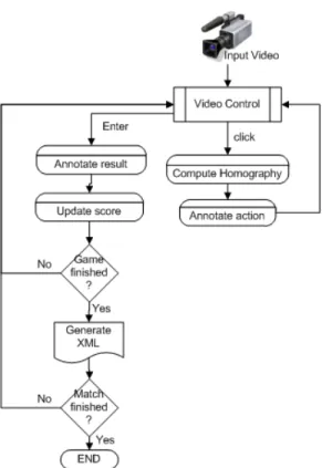
(30) 10. CHAPTER 2. ANNOTATION SYSTEM. 2.1. System Description. 2.1.1. Introduction. The initial approach was to design and develop a system able to capture automatically all needed variables. The University of Surrey had developed a similar system [11]. However, after using it for a short while, it was concluded that in order to obtain reliable and robust data, we would need to implement purpose-built system. The reasons for this are listed below: • Even though the University of Surrey’s system was able to recognize and classify the forehand and backhand strokes [50, 54], the results were only correct less than 60% of the time. Also, the granularity offered was not enough for a serious tactical analysis, which would need at least ten categories. • The ball trajectory results [74, 75] were better than the stroke detection ones, although it wasn’t 100% accurate due to the fact that only one camera was used and some occlusions were unavoidable. • The processing speed was very slow, taking more than one hour to analyze a few points. For these reasons and in order to ensure almost 100% data accuracy, that would enable us to identify correct strategic patterns, it was decided to implement our own system.. 2.1.2. System Design. The system has been designed to work with normal speed, low resolution cameras and broadcast sequences, as opposed to other systems that employ several high speed cameras[51]. On an average, the video sequences to analyze show the following characteristics: • Image: 640 x 480 pixels • Frame Rate: 25 frames per second The following figure depicts the main modules of the annotation system: A brief description of these modules can be found below. The Compute Homography module, however, will be further explained in the following sections..
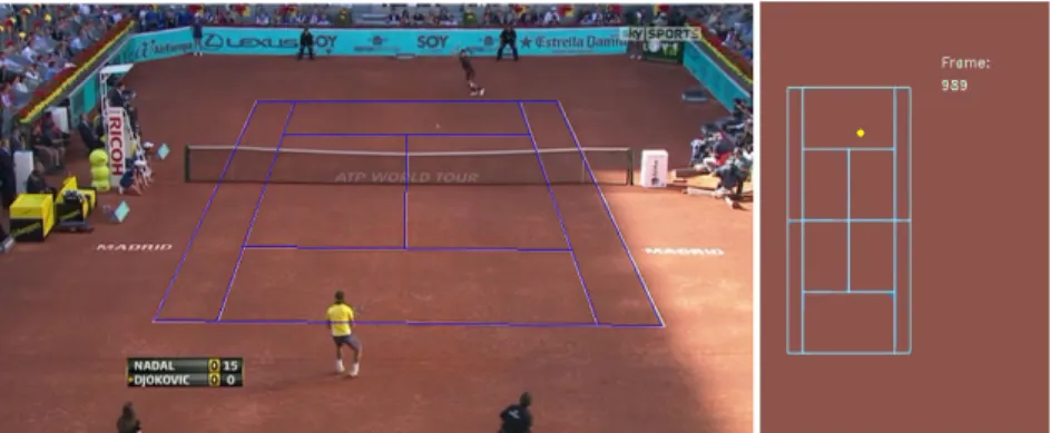
(31) 2.1. SYSTEM DESCRIPTION. 11. Figure 2.1: Data Capture and Annotation System. Video Control This module is in charge of playing the recorded broadcast video as well as offering an interactive interface with the user. This interface enables the user to play frame by frame, to fast-forward, to play backwards, control the playing speed and pause the recording. This module is also responsible for sending the selected frame to the Compute Homography module, which will process it and will return the real coordinates on the reference court model of the mouse position clicked on the broadcast image. This position is also visualized on the computer screen in a small representation of the tennis court for a quick correctness check.. Annotate Result This module assigns a winner to the point just played and registers the reason for its completion. The system allows the following options:.
(32) 12. CHAPTER 2. ANNOTATION SYSTEM. Figure 2.2: Ball position in broadcast image and in reference court • Winner. Shot that is not reached by the opponent and wins the point. • Forced error. Error caused by the opponent’s good play or attack. • Attacking Error. Error caused when the player attempts to attack the opponent. • Unforced error. Error that cannot be attributed to any factor other than poor execution by the player.. Annotate Action This module assigns a label or tag to the annotated position. Depending on the situation, different tags have been created. Table 2.1 shows the tags allowed by the system for the different types of strokes, and Table 2.2 shows the tags used to describe the status of the ball.. Update Score On of the most important variables to characterize the behavior of a player at a specific point in time is the score at that very moment. The implemented system uses this module to keep track of the score and automatically updates it after each point. The only information passed to this module is whether the match will be played to a maximum of 3 sets or 5 sets, and whether a tie-break will be permitted in the last set..
(33) 2.1. SYSTEM DESCRIPTION Tag FS SS FH FHS BH BHS VOL SM LOB DSH. 13. Description First Serve Second Serve Forehand (top spin or flat) Forehand sliced Backhand (top spin or flat) Backhand sliced Volley (forehand or backhand) Smash Lob (forehand or backhand) Dropshot (forehand or backhand). Table 2.1: Types of strokes annotated Tag NET BIN BOUT HBIN ME. Description Ball hits the net Ball bounces inside the court Ball bounces outside the court Hypothetical position where the ball would bounce Ball has not been hit correctly Table 2.2: Ball status. Generate XML At the end of each game, the system generates an XML file with all the captured information. The reason to generate a file for each game is because it allows easily to resume the annotation where we stopped it and avoids a possible loss of data in case of an unexpected error. On the other hand, we decided to separate the capture and annotation functionality from the analysis and data mining function. This way, one team could focus on the data gathering function on relatively standard PCs, where another team can explore the pattern identification in more powerful servers. The XML structure is as follows: <game> <sets_won_by_1></sets_won_by_1> <sets_won_by_2></sets_won_by_2>.
(34) 14. CHAPTER 2. ANNOTATION SYSTEM. <set5_p1></set5_p1> <set5_p2></set5_p2> <set4_p1></set4_p1> <set4_p2></set4_p2> <set3_p1></set3_p1> <set3_p2></set3_p2> <set2_p1></set2_p1> <set2_p2></set2_p2> <set1_p1></set1_p1> <set1_p2></set1_p2> <games_p1></games_p1> <games_p2></games_p2> <point> <server></server> <points_p1></points_p1> <points_p2></points_p2> <rally> <frame></frame> <action></action> <x></x> <y></y> </rally> (...more rallies...) <point2></point2> <outcome></outcome> </point> (...more points...) </game>. Compute Homography. This module is responsible for calculating the reference court coordinates of any location selected on the broadcast image. It also performs the player and court tracking. Its functioning will be described in detail in the following section..
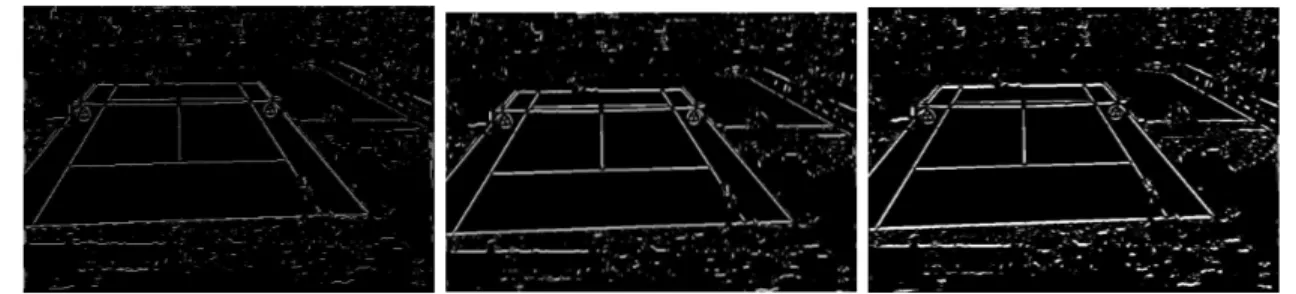
(35) 2.2. PRE-PROCESSING. 15. Figure 2.3: Annotation system overview. 2.1.3. High Level Overview. As mentioned above regarding the analysis of sports videos, the players’ positions as well as the ball bouncing positions have a great semantic importance, since these positions and their tracked movements provide information about the actions displayed on the court. For this analysis, it is necessary to calculate these positions on a reference model. In the next sections, we present a number of algorithms to achieve automatic calibration and tracking. These algorithms could apply to several sports providing a sufficient number of lines or references are present on the image. Figure 2.3 shows the main stages of the annotation system implemented. Figure 2.4 shows some of the logic and module dependencies from a high level point of view.. 2.2. Pre-Processing. The main purpose of this step is to extract a number of straight lines from the input frame, resulting in a set of court line candidates. The International Tennis Federation (ITF) dictates1 that all lines of the court shall be of the same color clearly contrasting with the color of the surface. In our analysis, all court lines studied were white. However, since they were not the only white objects in the images, a set of additional filters was needed. These filters will be described in the following sections and include a luminance filter to identify the white pixels on the image and discard the rest, a texture filter to remove white textured areas not belonging to court lines, i.e. white logos or white t-shirts, a linearity filter that ensures that all court lines candidates are nor wider that certain threshold and finally, we apply the probabilistic Hough transform due to its smaller computational cost and robustness on low quality images to find all the lines and intersections present in the image. 1. http://www.itftennis.com/technical/rules/index.asp.
(36) 16. CHAPTER 2. ANNOTATION SYSTEM. Figure 2.4: High level flowchart for the homography calculation and tracking.
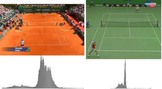
(37) 2.2. PRE-PROCESSING. 2.2.1. 17. Luminance Filter. Since the tennis court lines are white or light color, we apply an initial filter to remove the image pixels that do not hold this property. For this, as suggested by [23], we classify each image pixel as a possible line candidate based on its luminance, which is defined as: Y = 0.299 ∗ R + 0.587 ∗ G + 0.114 ∗ B. (2.1). In this way, if the value of the luminance on a pixel, Y (x , y) is greater than a specific threshold σy , then this pixel is considered a line candidate l (x , y) = 1 , otherwise the pixel is discarded: ( l (x , y) =. 1. if Y (x , y) ≥ σy. 0. otherwise. (2.2). Farin et al.[19, 20] propose a fixed threshold σy = 128 for all types of images. However, our tests have proved that an adaptive threshold value was fundamental in order for this filter to work properly on different light conditions, surface types of court colors. To this end, we first calculate the histogram of the image on a gray scale, but to avoid that the public or the stadium contaminates the result, we crop the image and only use a central section over which we calculate the histogram. The following Figures 2.5, 2.6 show several histograms for different surfaces and different lighting conditions. These histograms, which are calculated using 256 bins, show the presence of one or more peaks (the presence of two peaks is always a signature of grass courts) that indicate the most frequent luminance colors on the image processed. Therefore, the identification of an appropriate luminance threshold cannot be fixed for all frames in order to obtain good results. Our tests indicate that the following threshold definition allows for a luminance filter that works correctly under any lighting condition or court surface, making in turn, the calculation of the adaptive threshold an automatic process: σy := arg max {y | h(y) ≤ 0.7 ∗ hmax (ymax ) ∧ y ≥ ymax } y. (2.3). where h(y) is the histogram value for the bin y and ymax is the value of y for the maximum histogram value. See Figure 2.7..
(38) 18. CHAPTER 2. ANNOTATION SYSTEM. Figure 2.5: Histograms of the images’ central area for a clay court (left) and a one-color hard court (right). Figure 2.6: Histograms of the images’ central area for a two-color hard court (left) and a grass court (right). Figure 2.7: Luminance threshold calculation.
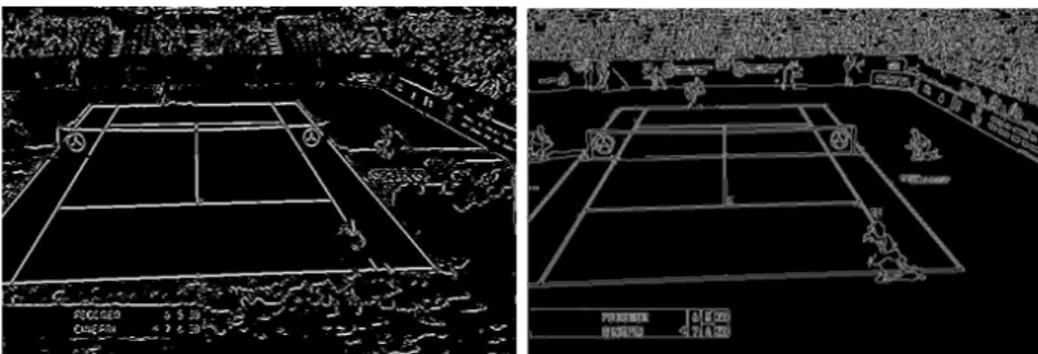
(39) 2.2. PRE-PROCESSING. 2.2.2. 19. Texture Filter. The previous luminance filter successfully removes the majority of the colors that compose the tennis court surface. However, the pixels that belong to the players’ light colored tshirts, or the white areas of the stadium or the sponsors logos are still considered to be line candidates. An initial attempt to detect tennis court lines through the Canny filter [42] resulted in a number of false positives (see Figure 2.9 right). To avoid this, we had to remove the white pixels in all textured regions, and this was done by means of the structure tensor. The structure tensor is a tool that encodes the structure information around a point and provides information about the maximum signal variation direction and its orthogonal direction [7]. The tool has been used in all kind of applications, such as: edge detection, corner detection, structure analysis, optical flow estimation and especially texture analysis. In the 2D case, the structure tensor S , also known as autocorrelation matrix, calculated for each pixel candidate around a window of pixels of dimension sp is defined as follows: P ∂I 2 P ∂I ∂I ( ∂x ) ∂x ∂y sp sp S = P P ∂I 2 ∂I ∂I ( ) ∂x ∂y ∂y sp. (2.4). sp. In our case, we have calculated the structure tensor for each pixel candidate around a window of pixels of dimension sp = 7 × 7 . The calculation of the derivatives is done through a Sobel operator of size 3 × 3 pixels which combines a Gaussian filter to smooth out the result and make it more robust against noise. Other methods exist to estimate the structure tensor based on a set of quadratic filters along with an analysis in the frequency domain, or more recently, non-linear versions of gradient based methods [7]. The calculation of the eigenvalues and eigenvectors of this matrix provides information about the local structure of the image. Specifically, if both eigenvalues λ1 , λ2 (λ1 ≥ λ2 ) are big, this means a textured area. If one eigenvalue is big and the other one small, it means that an edge with a certain orientation exists [20, 72]. We will use these properties as the criteria to remove textured areas and allow only the pixels that belong to straight lines. Our tests have shown that the next condition satisfies all requirements: λ1 > 5 · λ2. (2.5).
(40) 20. CHAPTER 2. ANNOTATION SYSTEM. Figure 2.8: Image after applying luminance filter (left) and the result after applying a texture filter with sp = 7 × 7 (right). Figure 2.9: Image after applying a texture filter with sp = 3 × 3 (left) and image after applying the Canny filter (right). Figures 2.8, 2.9 shows the result after applying this filter.. 2.2.3. Linearity Filter. After the previous filters have been processed, we apply a further constraint. We exploit the property of court lines not measuring more than τ pixels wide. This way, we check if there are pixels at a distance of τ pixels around the candidate pixel whose luminance is darker than the pixel under analysis. As suggested by Farin et al. [20], the threshold value for the luminance difference was set as σd = 20. Therefore, following Equation 2.2, we further consider a pixel as a line candidate l (x , y) = 1 or not l (x , y) = 0 , according to the.
(41) 2.2. PRE-PROCESSING. 21. Figure 2.10: Image after applying the linearity filter. τ = 1 (left) τ = 3 (center) and τ = 5 (right) following condition: 1 l (x , y) = 1 0. if Y (x , y) − Y (x − τ, y) > σd. ∧. Y (x , y) − Y (x + τ, y) > σd. if Y (x , y) − Y (x , y − τ ) > σd. ∧. Y (x , y) − Y (x , y + τ ) > σd (2.6). otherwise. Although Farin et al. suggests a value of τ = 8 pixels, our tests showed that the optimum value was τ = 3 pixels. Smaller values resulted in the removal of the top court lines (due to the camera perspective) and larger values brought about wider lines that would be treated by the Hough filter as multiple lines. Figure 2.10 shows the results for various values of τ .. 2.2.4. Probabilistic Hough Filter. The last pre-processing step involves parametrizing the lines identified on the image so they can be further analyzed. Since this analysis is based on line segments, it was decided to use the probabilistic Hough transform [36]. Other advantages of this method over the standard Hough transform include a smaller computational cost, more robustness on low quality images and a more control parameters [36, 5, 41]. The control parameters chosen for the probabilistic Hough transform for our particular scenario are the following: • Segment length ≥ 37 pixels • Space between segments of the same line so they can be considered as one line ≤ 10 pixels.
(42) 22. CHAPTER 2. ANNOTATION SYSTEM. Figure 2.11: Lines detected by the probabilistic Hough transform These parameters cover the requirements for tennis court lines, although they could be easily tuned to detect the lines in other sports such as soccer or volleyball. Figure 2.11 shows the result of applying the probabilistic Hough transform to Figure 2.8 on the right. Note. each segment has been displayed with a different color.. 2.2.5. Selection of the Main Lines. Usually, the result of applying the Hough transform is not going to be as clean as Figure 2.11. Most of times, specially in clay courts, the result obtained will consist of a number of segments with different lengths along the direction of the lines that define the tennis court (see Figure 2.12). However, it is necessary to extract the main lines from these segments for further analysis. A first step to obtain the main lines is to find groups of similar segments. To do so, we loop through all segments returned by the Hough filter and find groups of segments that verify the following condition: • The angle between the segments is < 3◦ • The distance between segments is ≤ 10 pixels This way, all the segments that belong to the same line are grouped together. The next step is to extract a single line from each group of segments. To do so, we have considered two options and both have been implemented. A first approach consists of locating the.
(43) 2.2. PRE-PROCESSING. 23. Figure 2.12: Detected segments along the lines. farthest points of the segments of a group and then join them together to produce a single line. The main advantage of this method, which was the first one to implement, is its speed. However, it has a weakness, since it needs the farthest points to be part of the main line and this was not always the case. Therefore, the second approach uses all the segments of the group in order to finding the main line. We do so by means of least squares linear regression analysis as described below.. Ordinary Least Squares Linear Regression In this method, we try to find a line that minimizes the distance from each of the segment’s farthest points. We do this by resolving a system of linear equations for each of the segments of each group: n X. Xij βj = yi ,. (i = 1, 2, . . . , m). (2.7). j=1. where Xij and yi represent the m coordinates of each of the segment’s farthest points, and m = 2 × ns , being ns the number of segments found for each group. βj represent the parameters of the approximation function and since we are trying to find a line, then n = 2..
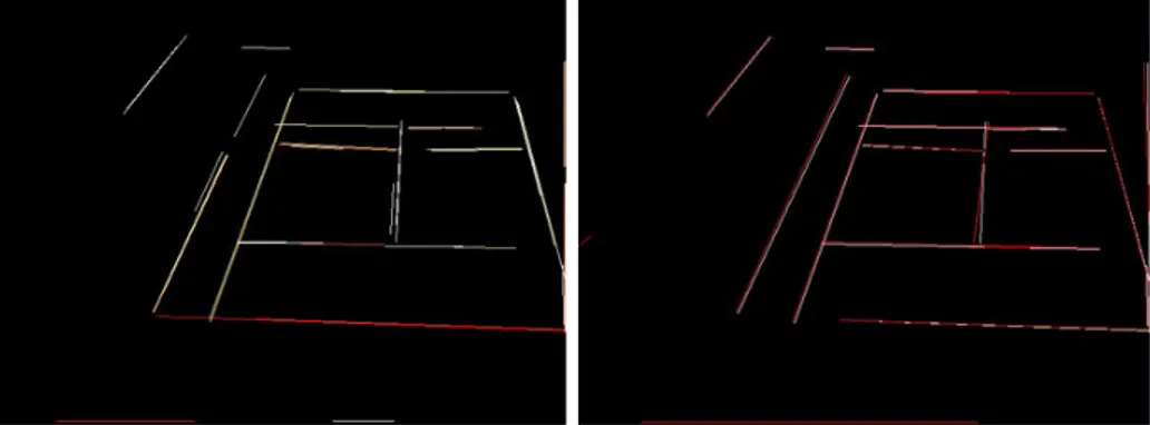
(44) 24. CHAPTER 2. ANNOTATION SYSTEM The previous equation can be written in matrix notation as: Xβ = y. (2.8). The result of solving this equation system by singular value decomposition is a line that takes into account all segments’ farthest points and minimizes their distance to it. Nevertheless, it became apparent that not all segments should contribute equally to the definition of the line. Usually, the longest segments are the most representative and the ones that should have a larger weight when identifying the resulting line.. Weighted Least Squares Linear Regression The previous method assumes that all residuals resulting from each of the equations that define the segments have the same variance and they are uncorrelated [45]. However, as mentioned above, the longest segments should contribute more towards the definition of the main line. To achieve this, we use weights adjusted depending on the length of each segment. There are two possible options: • To use a weighted matrix and then solving the system of equations. In this case, the diagonal matrix W is defined using the length of each segment: (X T W X)β̂ = X T W y. (2.9). • Alternatively, we could use equidistant points in each segment depending on its length, so that longer segments contribute with more points to the definition of the line. In our tests, a sampling of 30% of the total length of a segment provided good results without penalizing the process. As a summary for all these approaches, Figure 2.13 shows the results of applying the previous methods. The figure on the left shows the segments obtained after applying the Hough filter. The figure on the right shows the outcome of the main line selection process: lines in red were obtained joining directly the segment’s farthest points, whereas white lines were obtained after applying weighted least squares. It is noticeable on the vertical line in the center that the regression method outperforms the first initial approach..
(45) 2.3. AUTOMATIC CALIBRATION OF BROADCAST IMAGES. 25. Figure 2.13: Main line selection after applying different methods Line Classification Once all the main lines on the broadcast image have been identified, they are sorted into two sets. One set contains all the horizontal lines, while the other set consists of the vertical lines. Candidate lines are classified as vertical if their angle is less than 25◦ and horizontal otherwise.. 2.3. Automatic Calibration of Broadcast Images. The main purpose of this stage is to implement the appropriate algorithms to: a) relate the main lines detected during the preprocessing step to the court lines of a reference model, and b) find the geometric transform that converts the broadcast image under analysis into a projected one so that any point on the original image can be referenced back to a court model.. 2.3.1. Previous Work. The initial proposed systems [59] needed to manually select four lines in order for the process to identify the rest. Also, the geometric transform were based on a simplified camera model that only considered the tilt, the distance from the camera to the court and the focal distance. Calvo et al. [6] used the Hough transform to detect the court lines but they employed heuristics to assign the detected lines to reference model based on several assumptions. Recently Farin et al. [20] proposed a system more robust to occlusions also based on the Hough transform. His method used a combinatorial search to establish the.
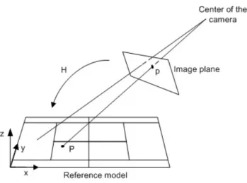
(46) 26. CHAPTER 2. ANNOTATION SYSTEM. correspondence between the image lines and the reference model. However, both the Hough transform and the combinatorial search were computationally expensive. For this reason, Farin proposed later a modification to his system [19], where he substituted the Hough transform by RANSAC-based line detector and he tried to establish the correspondences between the image lines and the reference model using two line segments instead of the four segments used originally. Finally, Hayet et al. [29] suggested an interesting improvement on the correspondence mapping based on geometric invariants. This allowed first to calculate the homography matrix using only two points (instead of four) and secondly, to provide more robustness to large occlusions. The system implemented in this thesis is mostly based on the projective geometry system proposed by Hayet et al.. 2.3.2. Homography. The camera model for perspective images of planes has been studied in detail before[16, 27]. Points on a reference plane are mapped to the points on the image by a plane projective transformation or homography. If we denote the coordinates of the points on the reference plane as homogeneous vectors P = (X, Y, 1)T , and the coordinates of the points on the image plane as homogeneous vectors p = (x, y, 1)T , then this homography relationship can be described as: P = Hp. (2.10). where H is a 3 × 3 homogeneous matrix which includes a scale factor. X h11 h12 h13 x Y = h21 h22 h23 y 1 1 h31 h32 h33. (2.11). In order to resolve 2.11, a system of equations with eight variables2 , it is sufficient to find four correspondences between the image and the reference model with the condition that three of them cannot be collinear points. 2. Since this is a scale invariant homogeneous matrix, and only ratios are important, the number of variables can be reduced from nine to eight..
(47) 2.3. AUTOMATIC CALIBRATION OF BROADCAST IMAGES. 27. Figure 2.14: Transformation between the image plane and the reference plane However, those correspondences are not known a-priori. Therefore, a list of hypothesis will have to be generated and evaluated by the system. Unfortunately, this process of generation/evaluation has two major weaknesses: • If only one of the four correspondences is wrong, the system will have to re-calculate the matrix H. Also, the system will not know which them is the wrong one, allowing this correspondence in further hypothesis evaluations. • The solution to the system of equations to obtain H is computationally expensive (it is done by singular value decomposition), especially if we need to make this calculation for each hypothesis evaluation. Hayet et al. [28, 29] proposal avoids the calculation of H as an evaluation method if we know the vanishing points. In this way, only two correspondences are needed instead of four, increasing the speed and the efficiency of the algorithm. We will describe this algorithm in the next section. Radial Distortion Although the matrix H does take into account both the internal parameters of the camera (such as the focal length, the position of the camera’s principal point, the aspect ratio and the skew) and the external ones (such as rotation and translation) [13], it does not compensate the nonlinear radial distortion which becomes apparent when the focal length.
(48) 28. CHAPTER 2. ANNOTATION SYSTEM. decreases [27]. The following equation shows an approximation function that corrects this problem when we assume a two-parameter radial distortion model and we ignore tangential distortion [51, 65]: f (r) = r + k1 r3 + k2 r5. (2.12). where ki are the radial distortion coefficients and r is the distance of the image coordinates to the center r2 = x2 + y 2 . Therefore, an estimation of the ki coefficients is enough to compensate camera lens distortions for the majority of practical applications. Moreover, in cases where narrow-angle cameras capture scenes far from the camera (which is our case), an approximation of the radial distortion can be obtained by simply calculating the k1 parameter. Previous work on tennis broadcast videos [11] suggest a value for k1 as: k1 = 2 × 10⁻⁷. (2.13). This value has been used for all sequence frames giving satisfactory results.. 2.3.3. Fast Projection Algorithm. Since we are working with a set of orthogonal lines, all lines on the tennis court converge either on the horizontal vanishing point or the vertical vanishing point. However, usual tennis broadcast videos place the camera at the end of one of the sides. This makes that the service and base lines are almost horizontal (see Figure 2.15).. Figure 2.15: Vanishing points for a typical broadcast perspective Therefore, the vertical lines identified at the end of the pre-processing phase (side lines and center lines) converge on a vertical vanishing point pv , whereas the horizontal lines.
(49) 2.3. AUTOMATIC CALIBRATION OF BROADCAST IMAGES. 29. Figure 2.16: Cross Ratio definition (base lines and service lines) converge ad infinitum, ph ∼ ∞. Calculation of pv The calculation of the vertical vanishing point is a RANSAC-based algorithm [21] which finds all vertical lines that converge “near” a possible vertical vanishing point. After that, an overdetermined system of equations is resolved using least squares. Because not many vertical lines are usually detected in our application, rather than choosing random vertical lines for a number of times (generic RANSAC algorithm), we iterate all possible combinations of vertical lines3 . The result of this algorithm is a set of vertical lines whose intersections are within a range of 3 pixels. All vertical lines that do not comply with this condition are removed from the final consensus (this eliminates all the vertical lines detected by the Hough algorithm which are not court lines). Once we have selected the set of vertical lines which do converge within 3 pixels, we use least squares to determine the most accurate vanishing point. The system of equations includes the linear equations of each of the lines that are part of the final consensus. The method used to resolve the linear system Ax = B was through singular value decomposition (SVD). The Cross Ratio Projective transformations do not maintain distances or distance ratios, however, a ratio of ratios or cross ratio of lengths on a line is maintained. This is the most important invariant in projective transformations [27]. 3. Even if we had 20 vertical lines, the number of possible combinations would be just 190. However, usually, no more than 6 vertical lines are detected after the pre-processing step..
(50) 30. CHAPTER 2. ANNOTATION SYSTEM The cross ratio can be defined for four collinear points or four concurrent lines. For the. points displayed in Figure 2.16, the cross ratio is defined as: XRatio =. |AB||CD| |A0 B 0 ||C 0 D0 | = 0 0 0 0 |AC||BD| |A C ||B D |. (2.14). As mentioned above, it is advisable not to compute the homography matrix H to evaluate each hypothesis because of its performance implications. Now, and once pv and ph are known, we can use the invariance property of the cross ratio to calculate the projection of any point on the reference model on to the image projective perspective.. Figure 2.17: Terminology used in fast projection Let us consider Figure 2.17, let us assume we want to evaluate hypothesis h = (p1 , P 1; p2, P 2), which includes two correspondences between the image plane and the reference model. The objective is to find the position of point p on the image plane, knowing its position P on the reference model. To do so, we calculate the cross ratio of the line which includes the four points (Y, Y2 , Y1 , Pv ) and its projection (y, v2 , v1 , pv ), where Y is the ordinate of point P on the y-axis, Y2 is the ordinate of point V2 on the y-axis, Y1 is the ordinate of point V1 on the y-axis. We obtain: XRatioA (p, v2 , v1 , pv ) =. pv2 v1 pv pv1 v2 pv. (2.15). Y − Y2 Y − Y1. (2.16). XRatioB (Y, Y2 , Y1 , Pvy ) =. XRatioA = XRatioB. (2.17). On the other hand, Figure 2.18 shows the points (p, v2 , v1 , pv ) on the projected image:.
(51) 2.3. AUTOMATIC CALIBRATION OF BROADCAST IMAGES. 31. Figure 2.18: Line (p, pv ) on the projected image If we apply the Thales theorem, we obtain: py − v2y pv2 v2x − px = = pv1 py − v1y v1x − px. (2.18). By solving these equations, we obtain the value of p = (px , py ) for the initial hypothesis h = (p1 , P 1; p2, P 2). Finally, it is worth mentioning that even though we have taken the cross ratio of four points as a single vale, it varies depending on the order in which we take the points. There exist 4! = 24 possible permutations, although due to symmetries, there are only six unique values of the cross ratio. Table 2.3 shows the different possibilities. Case A Pv V1 V2 P. Case B Pv V1 P V2. Case C Pv V2 V1 P. Case D Pv V2 P V1. Case E Pv P V1 V2. Case F Pv P V2 V1. Table 2.3: Different cases when calculating the cross ratio Therefore, the calculation of the cross ratio for each of these cases allows to obtain the value of p = (px , py ) for each couple of points taken as a hypothesis h. We can denote this relationship as: p = Πh (P ) The next section will detail how the system generates these hypothesis.. (2.19).
(52) 32. CHAPTER 2. ANNOTATION SYSTEM. 2.3.4. Hypothesis Generation. Once we have the main line segments parametrized from the pre-processing phase and classified as vertical or horizontal, the first step to generate a list of hypotheses is to calculate all possible intersections between the vertical and the horizontal segments. Figure 2.19 shows the terminology used to denote each of the intersections on a tennis court.. Figure 2.19: Terminology used to denote the intersections on the reference model However, looking at each of these intersections on Figure 2.19, it is noticeable that some of them share the same shape. We can, therefore, classify them accordingly as per Table 2.4. Table 2.4 shows that there are only eight unique shapes or categories. The next step is to associate these eight shapes with each of the intersections found on the image, allowing for a small error margin. For instance, to find the corner “A”, we allow for the following possibilities:. Figure 2.20: Shapes allowed to classsify an intersections as type “A” Let us denote a correspondence as (pi , Pi ), where pi represents a point on the image, and Pi its correspondent point on the reference model. After the classification process, we can generate two lists of correspondences. The first one will include the correspondences gener-.
(53) 2.3. AUTOMATIC CALIBRATION OF BROADCAST IMAGES Intersection A B C D E F G H I J K L M N. Shape p q x y > > ⊥ ⊥ ` ⊥ a ` > a. 33. Category A B C D Tt Tt Tb Tb Tl Tb Tr Tl Tt Tr. Table 2.4: Classification of intersections according to their shape on the reference model ated by the actual intersections detected on the image, in other words, those intersections to which we could assign a shape or category. To generate the list of correspondences, we just need to take into account the different possibilities between intersections and categories shown in Table 2.4. On the other hand, and in order to make the system more robust, when none of the correspondences of the first list yields adequate results, a second list of correspondences is generated. This second list includes all possible intersections between all horizontal and vertical segments from the image. Note that this second list in only used in case of error since its evaluation is a lot more costly. Finally, we construct a list of hypotheses, where each hypothesis hk = (pi , Pi ; pj , Pj ) is made of each of the possible combinations between two correspondences: H = {hk }. 2.3.5. (2.20). Hypothesis Evaluation. The hypothesis evaluation consists of checking its ability to justify the results observed, i.e., the detected lines and intersections on the image. In this way, if {pi } is the set of intersections on the image and {Pj } is the set of intersections on the reference model, each.
(54) 34. CHAPTER 2. ANNOTATION SYSTEM. hypothesis hk = (pi , Pi ; pj , Pj ) is evaluated comparing the set {pi } with the set {Πh (Pj )}. Since the number of hypotheses to evaluate can be considerable, a RANSAC-based algorithm has been implemented. See Figure 2.21. input H, set of hypotheses; {pi }, set of intersections on the image; {Πh (Pj )}, set of projections of the model’s intersections {Pj } on the image under hypothesis h; output hk , hypothesis that better supports the results observed (larger number of coincidences found) {pi , Pj }, set of correspondences that hold under hypothesis hk begin coincidences := 0 iterations := 0 best number of coincidences := 0 while iterations < max iterations and coincidences < min coincidences Choose randomly a hypothesis h with two non-collinear correspondences foreach intersection {Pj } on the reference model Calculate its projection {Πh (Pj )} on the image foreach intersection {pi } if projection is within margin allowance error from any of the intersections {pi } and their categories coincide 1. coincidences + + 2. keep the correspondence if coincidences > best number of coincidences 1. best number of coincidences = coincidences 2. keep this hypothesis h 3. keep the correspondences iterations + + coincidences = 0 reset correspondences found return hk {pi , Pj } end Figure 2.21: Hypothesis evaluation algorithm. Our experimental tests have shown than the following values yield a good trade-.
(55) 2.3. AUTOMATIC CALIBRATION OF BROADCAST IMAGES. 35. off between speed and efficiency: max iterations = 200, min coincidences = 8 and margin allowance = 3 pixels. Therefore, the output of the algorithm would be the best two correspondences-hypothesis that produces the largest number of coincidences between the reference model and the intersections detected on the broadcast image. The output of the algorithm also provides a list with all the coincidences found under this hypothesis, i.e., all the correspondences {pi , Pj } verified. This way, if the number of verified coincidences is n, then we will obtain n + 2 verified correspondences (n < 12).. 2.3.6. Homography Matrix Calculation. As explained in section 2.3.2, the calculation of the homography matrix H will allow us to obtain the position on the reference model of any point selected on the broadcast image in a single operation. This is needed for the notational analysis introduced at the beginning of this chapter. Additionally, the matrix H also allows to obtain the projection of the reference model on the broadcast image, and therefore, enabling the system to be able track the court throughout a sequence of frames. Once the best hypothesis and the list of verified correspondences have been found as detailed in the previous section, we can now calculate the homography matrix. As mentioned in section 2.3.2, only four correspondences are needed in order to resolve the resulting system of equations, providing that three of them are not collinear. Thus, we need to select the four correspondences to be used out of the list of all possible correspondences found. These four points shall be chosen in a way that maximize the resulting polygon area to compensate for distortion errors. The method used to maximize the area and find the four correspondences which will be used to calculate the matrix H can be seen in Figure 2.22, which uses Jarvis’ algorithm [34] to compute the convex hull of a given set of points. Once the homography matrix has been calculated, we can use the projective transform P = Hp to find out the position on the reference model of any point selected on the broadcast image during the video playback. The resulting point, P = (X, Y, 1)T will be passed over to the video control module for its annotation and further analysis. We will also use the homography matrix to calculate the projection of the reference model intersections on the image frame. This will be used by the court tracking module to quickly calculate the new homography matrix in later frames. This projection calculation.
(56) 36. CHAPTER 2. ANNOTATION SYSTEM. input {pi , Pj }, set of verified correspondences under hypothesis hk ; output {pk , Pl } ∈ {pi , Pj }, set of four correspondences for which {pk } produces a max area; begin max area := 0 foreach possible combination of four correspondences 1. Find the convex hull of the four points chosen, numbering the vertices 2. Find the area by calculating its cross product P area = 12 3i=0 (xi yi+1 − xi+1 yi ) if area > max area 1. max area = area 2. Keep this combination of correspondences return {pk , Pl } end Figure 2.22: Algorithm to find the optimum four correspondences. is also direct: p = H −1 P. (2.21). Figure 2.23 shows the result of the identifying all court points (in green) and projecting them along with the court lines back onto the broadcast image using the homography matrix.. 2.3.7. Results. The detection algorithms have been applied to a total of 2,143 frames from several TV DVB broadcast tennis games converted to avi format using the MPEG-4-based XviD codec. The analyzed games cover all surface courts (hard court, grass court and clay court) and under several lighting conditions. Figures 2.24, 2.25, 2.26, 2.27 show several specially difficult frames. These figures show the use of the homography matrix to project (warp) the image on the reference model. Figure 2.24 shows a large shade that darkens most of the court line pixels, thus making difficult to detect the lines. In this case, the system calculates all possible intersections and successfully identifies a correct hypothesis. Figure 2.25 shows.
Figure
+7


Documento similar
To carry out this project successfully, the workflow has been divided into 4 categories: Data, Deep Learning, Machine Learning and Handcrafted Features. For the input of these
Another notable work in the identification of Academic Rising Stars using machine learning came in Scientometric Indicators and Machine Learning-Based Models for Predict- ing
En este sentido, tras mas de dos décadas compitiendo con nuevas reglas y materiales de juego, en esta investigación se plantea como objetivo describir la
The Health Belief Model (HBM) [3], the Theory of Reasoned Action (TRA) [4] or Planned Behavior (TPB) [5], the Information- Motivation-Behavioral Skills Model (IMB) [6], and
The data for learning self-regulation (higher values in this variable mean that the students used more strategies oriented to learning goals) is coming from the
In this work we address this issue and present a fundamental theoretical analysis of the dynamics and steady-state characteristics of lasing action in plasmonic crystals consisting
Tuning high-harmonic generation by controlled deposition of ultrathin ionic layers on metal surfaces
Under the action of the strong laser field, electrons can be extracted either from the topmost layers of Cu(111) and then injected into the NaCl bands (initial Cu-surface state) or
Figure 4 shows changes in the friction coefficient of the substrate and the coatings, according to the sliding distance, where the steady state is clearly seen. During this state
