Toward a climate-dependent paradigm of ammonia emission & deposition.

(1)

rstb.royalsocietypublishing.org

Research

Cite this article:

Sutton MA

et al

. 2013

Towards a climate-dependent paradigm of

ammonia emission and deposition. Phil

Trans R Soc B 368: 20130166.

http://dx.doi.org/10.1098/rstb.2013.0166

One contribution of 15 to a Discussion Meeting

Issue ‘The global nitrogen cycle in the

twenty-first century’.

Subject Areas:

environmental science

Keywords:

ammonia, emission, deposition, atmospheric

modelling

Author for correspondence:

Mark A. Sutton

e-mail: [email protected]

Electronic supplementary material is available

at http://dx.doi.org/10.1098/rstb.2013.0166 or

via http://rstb.royalsocietypublishing.org.

Towards a climate-dependent paradigm

of ammonia emission and deposition

Mark A. Sutton

1

_{, Stefan Reis}

1

_{, Stuart N. Riddick}

1,2

_{, Ulrike Dragosits}

1

_,

Eiko Nemitz

1

_{, Mark R. Theobald}

3

_{, Y. Sim Tang}

1

_{, Christine F. Braban}

1

_,

Massimo Vieno

1

_{, Anthony J. Dore}

1

_{, Robert F. Mitchell}

1

_{, Sarah Wanless}

1

_,

Francis Daunt

1

_{, David Fowler}

1

_{, Trevor D. Blackall}

2

_{, Celia Milford}

4,5

_,

Chris R. Flechard

6

_{, Benjamin Loubet}

7

_{, Raia Massad}

7

_{, Pierre Cellier}

7

_,

Erwan Personne

7

_{, Pierre F. Coheur}

8

_{, Lieven Clarisse}

8

_{, Martin Van Damme}

8

_,

Yasmine Ngadi

8

_{, Cathy Clerbaux}

8,9

_{, Carsten Ambelas Skjøth}

10,11

_,

Camilla Geels

10

_{, Ole Hertel}

10

_{, Roy J. Wichink Kruit}

12

_{, Robert W. Pinder}

13

_,

Jesse O. Bash

13

_{, John T. Walker}

13

_{, David Simpson}

14,15

_{, La´szlo´ Horva´th}

16

_,

Tom H. Misselbrook

17

_{, Albert Bleeker}

18

_{, Frank Dentener}

19

_{and Wim de Vries}

20

1_{NERC Centre for Ecology & Hydrology Edinburgh, Bush Estate, Penicuik EH26 0QB, UK} 2_{Department of Geography, Strand Campus, Kings College London, London WC2R 2LS, UK}

3_{Higher Technical School of Agricultural Engineering, Technical University of Madrid, Ciudad Universitaria s/n,} 28040 Madrid, Spain

4_{Izan˜a Atmospheric Research Center, Meteorological State Agency of Spain (AEMET), Santa Cruz de Tenerife 38071, Spain} 5_{University of Huelva, Huelva, Spain}

6_{INRA, Agrocampus Ouest, UMR 1069 SAS, 65 rue de St. Brieuc, 35042 Rennes Cedex, France} 7_{UMR INRA-AgroParisTech Environnement et Grandes Cultures, 78850 Thiverval-Grignon, France} 8_{Spectroscopie de l’atmosphe`re, Chimie Quantique et Photophysique, Universite´ Libre de Bruxelles (ULB),} 50 avenue F. D. Roosevelt, 1050 Brussels, Belgium

9_{Universite´ Paris 06, Universite´ Versailles-St. Quentin, UMR8190, CNRS/INSU, LATMOS-IPSL, Paris, France} 10_{Department of Environmental Science, Aarhus University, P.O. Box 358, Frederiksborgvej 399, 4000 Roskilde, Denmark} 11_{National Pollen and Aerobiology Research Unit, University of Worcester, Henwick Grove, Worcester WR2 6AJ, UK} 12_{TNO, Climate, Air & Sustainability, P.O. Box 80015, 3508 TA Utrecht, The Netherlands}

13_{US Environmental Protection Agency, Office of Research and Development, Research Triangle Park, 109 T.W.} Alexander Drive, Durham, NC 27711, US

14_{Norwegian Meteorological Institute, EMEP MSC-W, P.O. Box 43-Blindern, 0313 Oslo, Norway}

15_{Chalmers University of Technology, Department of Earth and Space Science, 412 96 Gothenburg, Sweden} 16_{Plant Ecology Research Group of Hungarian Academy of Sciences, Institute of Botany and Ecophysiology, Szent} Istva´n University, Pa´ter K. utca 1, 2100 Go¨do¨llo´´, Hungary

17_{Rothamsted Research, Sustainable Soils and Grassland Systems, North Wyke, Okehampton EX20 2SB, UK} 18_{Energy Research Centre of the Netherlands (ECN), P.O. Box 1, 1755 ZG Petten, The Netherlands} 19_{European Commission, DG Joint Research Centre, via Enrico Fermi 2749, 21027 Ispra, Italy}

20_{Alterra, Wageningen University and Research Centre, Droevendaalsesteeg 4, 6708 PB Wageningen, The Netherlands}

Existing descriptions of bi-directional ammonia (NH3) land–atmosphere exchange incorporate temperature and moisture controls, and are beginning to be used in regional chemical transport models. However, such models have typically applied simpler emission factors to upscale the main NH3 emis-sion terms. While this approach has successfully simulated the main spatial patterns on local to global scales, it fails to address the environment- and cli-mate-dependence of emissions. To handle these issues, we outline the basis for a new modelling paradigm where both NH3 emissions and deposition are calculated online according to diurnal, seasonal and spatial differences in meteorology. We show how measurements reveal a strong, but complex pattern of climatic dependence, which is increasingly being characterized using ground-based NH3 monitoring and satellite observations, while advances in process-based modelling are illustrated for agricultural and natu-ral sources, including a global application for seabird colonies. A future architecture for NH3 emission–deposition modelling is proposed that inte-grates the spatio-temporal interactions, and provides the necessary

(2)

foundation to assess the consequences of climate change. Based on available measurements, a first empirical estimate suggests that 58C warming would increase emissions by 42 per cent (28–67%). Together with increased anthropogenic activity, global NH3 emissions may increase from 65 (45–85) Tg N in 2008 to reach 132 (89–179) Tg by 2100.

1. Introduction

Ammonia (NH3) can be considered as representing the primary form of reactive nitrogen (Nr) input to the environment. In the human endeavour to produce Nrfor fertilizers, munitions and other products, NH3is the key manufactured compound, pro-duced through the Haber–Bosch process [1]. Synthesis of NH3is also the central step in the biological fixation of N2to pro-duce organic repro-duced nitrogen compounds (R-NH2), such as amino acids and proteins. When it comes to the decomposition of these organic compounds, ammonia and ammonium (NH4þ), collectively NHx, are again among the first compounds pro-duced. These changes lead to a cascade of transformations into different Nrforms, with multiple effects on water, air, soil quality, climate and biodiversity, until Nris eventually denitri-fied back to N2.

Although the behaviour of ammonia has long been of inter-est at both micro and macro scales [2], recent scientific efforts and policies have given it much less attention than other Nr forms. For example, under revision of the UNECE Gothenburg Protocol in 2012, the controls for NH3were the least ambitious of all pollutants considered, with a projected decrease in NH3 emission for the EU (between 2010 and 2020) of only 2 per cent, compared with reductions of 30 per cent for SO2 and 29 per cent for NOx(based on CEIP [3] and UNECE [4]).

In North America, India and China the expected trends are even more challenging. Figure 1 shows the relative changes in atmospheric Nrdeposition across the east of North America pro-jected for 2001–2020 [5]. Despite increases in traffic volume, the implementation of technical measures to reduce NOxemission from vehicles contributes an approximately 40 per cent reduction in oxidized nitrogen (NOy) deposition. By comparison, the mini-mal adoption of technical measures to reduce NH3 emission from agriculture is being offset by increased meat and dairy con-sumption, requiring more livestock and fertilizers, increasing NHxdeposition in some areas by greater than 40 per cent.

The combination of weak international commitments to miti-gate NH3and increasingper capitaconsumption represents one of the greatest challenges for future management of the nitrogen cycle [6,7]. The reality is that, rather than needing more Nrto sus-tain ‘food security’, in developed parts of the world high levels of Nrconsumption are being used to sustain ‘food luxurity’—the security of our food luxury. Ammonia must be a key part of the societal debate on these issues, where scientific advances in understanding and quantification are essential, especially as NH3emission is one of the largest Nrlosses.

Most NH3emissions result from agricultural production, and are strongly influenced by climatic interactions. In principle, according to solubility and dissociation thermodynamics, NH3 volatilization potential nearly doubles every 58C, equivalent to aQ10(the relative increase over a range of 108C) of 3–4. At the same time, NH3emission is controlled by water availability, which allows NHxto dissolve, be taken up by organisms and be released through decomposition. Considering these

interactions, NH3emission and deposition are expected to be extremely climate-sensitive. For example, will climate warming increase NH3emissions and their environmental effects, and to what extent will this hinder NH3mitigation efforts?

While substantial advances have been made in process-level understanding of NH3land–atmosphere exchange [8–14], these advances have not been fully upscaled at national, continental and global levels. Bi-directional models using the ‘canopy com-pensation point’ approach [10,15] have only been included to a limited extent in a few chemistry and transport models (CTMs) [5,16–18].

In addition, CTMs are still largely based on precalculated emission inventories. Under this approach, activity statistics are combined with emission factors to estimate annual emissions, which are mapped typically with relatively simple temporal dis-aggregation. The resulting fixed emission estimates are attractive to policy users in relation to reporting national emissions com-mitments. However, the approach fails to recognize that a warm-dry year would tend to give larger NH3emissions than a cold-wet year. At the same time, it does not address the short-term interactions relevant for risk assessment of NHx impacts [5,19,20].

To address these issues, this paper examines the relation-ships between climatic drivers and ammonia exchange processes. We first consider the magnitude of global NH3 emis-sions. Following consideration of the process relationships controlling NH3exchange, we show how studies of a natural NH3source (seabird colonies) can be used to demonstrate the climatic dependence of emissions and verify a global model. Finally, we outline a new architecture that sets the challenge for a new paradigm for regional modelling of atmospheric NHx as the basis for incorporating the effects of climate differences and climate change.

2. Ammonia emission inventories

The main reasons for constructing NH3emissions inventories have been to meet national-scale policy requirements and provide input to CTMs. Among the best studied national NH3inventories are those of the Netherlands [21], Denmark [22], the UK [23,24], Europe [25] and the US [5].

Although there is frequent debate on the absolute mag-nitude of national emissions and their consistency with atmospheric measurements [26], such inventories have allowed high-resolution CTMs to show a close spatial correlation with annual atmospheric NH3and NH4þconcentrations. In Europe, the inventories have focused especially on livestock housing and grazing, storage and spreading of manures, and from mineral fertilizers [27]. Less attention has been given to non-agricultural emissions including sewage, vehicles, pets, fish ponds, wild animals and combustion, which can contribute 15 per cent to national totals [28,29].

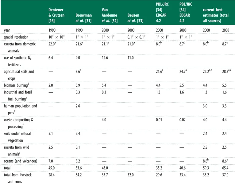
By comparison with the best national estimates, global NH3 emission inventories are much less certain. This reflects the wider diversity of sources and fewer underpinning data, com-bined with a paucity of activity statistics (e.g. animal numbers, bodyweights, diets, etc.). The contrast is illustrated between Den-mark, where 1 km resolution data on livestock numbers account for species sub-classes and abatement techniques [30], and other parts of the world, where such statistics often do not even exist. Recent global estimates of annual NH3emission are sum-marized in table 1. Dentener & Crutzen [16] were the first to

rs

tb.r

oy

alsocietypublishing.org

Phil

Trans

R

Soc

B

368:

20130166

(3)

1.4

(a) (b) (c)

N_r NH_x

NO_y

1.3 1.2 1.1 1.0 0.9 0.8 0.7 0.6 0.5 0.4

Figure 1.

Simulated changes in N deposition in eastern USA, showing the ratios for 2020/2001 (adapted from Pinder

et al

. [5]). (

a

) Oxidized N deposition,

(

b

) reduced N deposition and (

c

) total N deposition.

Table 1.

Comparison of global ammonia emission estimates (Tg N yr

21

).

Dentener

& Crutzen

[16]

Bouwman

et al.

[31]

Van

Aardenne

et al.

[32]

Beusen

et al.

[33]

PBL/JRC

[34]

EDGAR

4.2 PBL/JRC

[34]

EDGAR

4.2 current best

estimates (total

all sources)

year

1990

2000

2008

2000

2008

spatial resolution

10

8

10

8

1

8

1

8

1

8

1

8

0.1

8

0.1

8

1

8

1

8

1

8

1

8 excreta from domestic

animals

22.0

a

21.6

a

21.1

a

21.0

a

8.0

b

8.7

b

8.0

b

8.7

b

use of synthetic N

r

fertilizers

6.4

9.0

12.6

11.0 agricultural soils and

crops

—

3.6

c

—

21.6

a

24.7

a

25.2

a,c

28.3

a,c

biomass burning

d

2.0

5.9

5.4 —

4.4

5.5

4.4

5.5 industrial and fossil

fuel burning

e

—

0.3

0.3 —

1.3

1.6

1.3

1.6 human population and

pets

f

—

2.6 —

—

3.0

3.3 waste composting &

processing

f

—

4.0 —

0.01

0.02

4.0

4.4 soils under natural

vegetation

5.1

2.4 —

—

2.4

2.4 excreta from wild

animals

g

2.5

0.1 —

—

2.5

2.5 oceans (and volcanoes)

7.0

8.2 —

—

8.6

h

8.6

h

total

45.0

53.6

43.0 —

35.2

40.6

59.3

65.4 total from livestock

and crops

28.4

34.2

33.7

32.0

29.6

33.4

33.2

37.0

a

_{Includes emissions from grazing and land application of animal manure.}

b

_{Excludes emissions from land application of animal manure.}

c

_{Includes estimated direct crop emissions from foliage and leaf litter.}

d

_{Including savannah, agricultural waste, forest, grassland and peatland burning/ﬁres.}

e

_{Not including potentially high emissions from low-efﬁciency domestic coal burning [2].}

f

_{Rescaled by global population increase.}

g

_{The estimate of Bouwman}

_{et al.}

_{[31] is considered low given NH}

3

emissions from seabird colonies alone of 0.3 Tg N yr

21

[35].

h

_{Includes an upper estimate of 0.4 Tg N yr}

21

_{as NH}

x

from volcanoes based on an emission ratio of 15% NH

x

: SO

2

[2] and volcanic SO

2

emissions of

6.7 Tg S yr

21

[36].

rs

tb.r

oy

alsocietypublishing.org

Phil

Trans

R

Soc

B

368:

20130166

(4)

derive a global 108108NH3emission inventory for input to global CTMs. Bouwmanet al.[31] made a global NH3 inven-tory for the main sources at 1818 for 1990, while Beusen et al.[33] extended this for livestock and fertilizers.

One of the first points to note in the global comparison is that the source nomenclature is not well harmonized. Current standardization of inventory reporting by EDGAR (Emission Database for Global Atmospheric Research [34]) and the UNFCCC (United Nations Framework Convention on Cli-mate Change) focuses strongly on combustion sources and is less suited for sector analysis of agricultural emissions. It is, therefore, not easy to distinguish the main livestock sec-tors in the most recent inventories. According to Dentener & Crutzen [16], of 22 Tg NH3–N yr21 emitted from livestock, 65 per cent was from cattle and buffalo, with 13 per cent, 11 per cent, 6 per cent and 5 per cent, from pigs, sheep/ goats, poultry and horses/mules/asses, respectively.

The degree of agreement shown in table 1 (35–54 Tg N yr21₎ results partly from dependence on common datasets (e.g. Food and Agriculture Organization) and partly because of including different emission terms in each inventory. If all sources listed among the inventories are combined, this gives a total of 59 and 65 Tg N yr21for 2000 and 2008, respectively. These values are based on the recent estimates of EDGAR, combined with approximately 8 Tg yr21 _{from oceans and}

approximately 12 Tg yr21 _{from humans, waste, pets, wild} animals and natural soils.

These estimates should be considered uncertain by at least

+30% (based on propagation of likely ranges for input data, [33]), indicating an emission range of 46– 85 Tg N for 2008, although a formal uncertainty analysis on the full inventory has never been conducted. Apart from the uncertainties related to emission factors and climatic dependence, inaccur-ate activity data may introduce regional bias. For example, comparison of NH3 satellite observations (see §4) with a global CTM showed substantial underestimation by the CTM in central Asia [37], suggesting an under-reporting of animal numbers and fertilizer use in these countries.

Figure 2 shows that the regions of the world with highest emissions are mostly associated with livestock and crops. Because the available sector categorization does not distinguish arable and livestock sectors, the orange-shaded areas represent locations with a very strong livestock dominance. Biomass burn-ing is the main NH3source across much of central Africa, where estimated NH3emissions reach levels similar to peak agricultural values of India and China. Inclusion of the recent estimates of Riddicket al.[35] shows how seabird colonies are a significant NH3 source for many subpolar locations. These global maps hide substantial local variability, as illustrated for the UK in the electronic supplementary material, figure S1.

60°N

annual ammonia emissions kg Nha–1

<1 >1.0–2.5 >2.5–5.0 >5–10 >10–25 >25

dominant NH₃ source background seabirds agricultural soils

biomass and agriculture waste burning other non-agricultural

manure management no dominant source

60°N

40°N

20°N

0°

20°S

60°N

40°N

20°N

0°

20°S

40°S

80°S 60°S 60°N

60°S 40°S

60°S

120°E

30°W 0° 60°E 180°

90°W 150°W

120°E

30°W 0° 60°E 180°

90°W 150°W 80°S 60°S

80°N 150°W 90°W 30°W0° 60°E 120°E 180°

Figure 2.

Spatial variability in global ammonia emissions based on JRC/PBL [34] (livestock, fertilizers, biomass burning, fuel consumption) and Riddick

et al.

[35]

(seabirds). Emissions from oceans, humans, pets, natural soils and other wild animals (table 1) are not mapped. High-resolution maps for the UK are given in the

electronic supplementary material, figure S1.

rs

tb.r

oy

alsocietypublishing.org

Phil

Trans

R

Soc

B

368:

20130166

(5)

It must be emphasized, however, that these global esti-mates only take climate factors into account in a limited way. For emissions from fertilizer and manure application, climate has been partly considered by grouping datasets into major temperature regions [38], whereas Riddicket al.[35] applied a simple temperature function. However, the published global inventories do not model NH3 at a process level in relation to changing meteorological conditions. In addition, bi-directional NH3 fluxes from crops, sparsely grazed land and natural vegetation provide a particular challenge, because both the magnitude and direction of the flux varies according to ecosystem, management and environmental variables.

3. Concepts for modelling ammonia land –

atmosphere exchange

Current conceptual frameworks on NH3exchange show how fluxes respond to short-term variation in environmental con-ditions, and hence to long-term climate differences. This can be illustrated by the case of bi-directional exchange between plant, soil and atmosphere.

Ammonia fluxes are often considered as representing a potential difference between two gas-phase concentrations constrained by a set of resistances. At its simplest, the concen-tration at the surfacex(zo0), wherez_o0is the notional height of

NH3exchange, is contrasted with the concentrationx(z) at a reference heightzabove the canopy, with the total flux (Ft):

Ft¼

½xðzo0Þ xðzÞ

½RaðzÞ þRb

; ð3:1Þ

whereRa(z) andRbare the turbulent atmospheric and quasi-laminar boundary layer resistances, respectively [10,15]. A well-known variant of this approach, applicable only for deposition, assumes that the concentration at the absorbing surface is zero, so that any limitation to uptake can be assigned to a canopy resistance (Rc):

Ft¼

½0xðzÞ

½RaðzÞ þRbþRc

; ð3:2Þ

where an associated term, the deposition velocity, is defined as

VdðzÞ ¼ ðRaðzÞ þRbþRcÞ1¼ Ft=xðzÞ:It is possible to

inter-pret NH3flux measurements according to either view. This is illustrated in the electronic supplementary material, figure S2, which summarizes results from a year of continuous hourly NH3flux measurements over an upland moorland in Scotland [39]. Applying equation (3.1) to the flux measurements demon-strates the relationship betweenx(zo0) and canopy temperature,

while applying equation (3.2) to calculateRcfor the same data-set is necessarily restricted to periods where deposition was recorded. These two approaches represent different views of the factors driving and constraining the net flux.

The value of x(zo0) at the surface is proportional to a

ratio termed G¼[NH4þ]/[Hþ], where according to the thermodynamics:

x¼ 161 500

Texpð10 380=TÞ_½_NHþ

4=½H

þ; ð3:3Þ

withT in Kelvin [15]. The existence of bi-directional fluxes illustrated in the electronic supplementary material, figure S2, shows that calculatingx(zo0) provides the more general

solution, whereas its increase according to thermodynamics (fitted line, Q10¼3 –4) suggests that it reflects a process

reality. An exception is seen in frozen conditions, whereRc may be better suited to describe slow rates of deposition, as seen also for other gases [40]. However, considering the full year of measurements, the clear relationship with x(zo0) in

electronic supplementary material, figure S2, illustrates the weakness of sole reliance on theRcandVdapproach typically applied in CTMs.

The approach described above outlines the most simple situation. In reality, each of surface concentrations, resistan-ces and even capacitanresistan-ces can be used to simulate NH3 exchange, whereas both advection and gas–particle inter-actions can also affect fluxes [11,41,42]. A framework to consider the key issues at the plot scale is shown in figure 3, lar-gely based on Suttonet al. [10,43], Flechard et al. [44] and Nemitzet al.[15]. In this development of the resistance analogy, the central term is the ‘canopy compensation point’ (xc), which is identical tox(zo0) whenF_t¼0. This is contrasted with the

‘stomatal compensation point’ (xs), which is the NH3gas con-centration at equilibrium with [NH4þ]/[Hþ] in the apoplast, Gapo. Available data suggest only modest diurnal variation in Gapo [11]. The main challenge, therefore, is to estimate the larger differences inGapoowing to management, plant species and seasonality [45–47]. This can be investigated by including NH3cycling in models of ecosystem dynamics and agricultural management [11,18,48–50].

The most widely used approach to simulate NH3 exchange with the cuticle is to assume that deposition is constrained by a cuticular resistance (Rw) [10,15]. General parametrizations of this response to humidity and to NH3:

atmosphere

litter/soil canopy

scheme 1 scheme 2

R_b

R_a

R_w R_d

C_d

K_r

Q_d

R_s R_ac

ca

cI

cc

Gapo

cs

cd

Figure 3.

Resistance analogue of NH

3

exchange including cuticular, stomatal

and ground pathways. Two schemes for cuticular exchange are illustrated:

scheme 1, steady-state uptake according to a varying cuticular resistance

(

R

w

); scheme 2, dynamic exchange with a pool of NH

4þ

treated with varying

capacitance (

C

d

) and charge (

Q

d

). Other resistances are for turbulent

atmos-pheric transfer (

R

a

), the quasi-laminar boundary layer (

R

b

), within-canopy

transfer (

R

ac

), cuticular adsorption/desorption (

R

d

) and stomatal exchange

(

R

s

). Also shown are the air concentration (

x

a

), cuticular concentration

(

x

d

), stomatal compensation point (

x

s

), litter/soil surface concentration

(

x

l

) and the canopy compensation point (

x

c

). Exchange between aqueous

NH

4þ

pools is shown with dashed lines, including

K

r

, the exchange rate

between leaf surface and apoplast.

rs

tb.r

oy

alsocietypublishing.org

Phil

Trans

R

Soc

B

368:

20130166

(6)

acid-gas ratios have been developed ([15,46,51]; electronic supplementary material, figure S3; figure 3, scheme 1). These approaches have the advantage of relative simplicity, but only represent a steady-state approximation to a dynamic reality, where both adsorption (favouring net deposition) and desorption (favouring emission) occur in practice.

This dynamic view can be addressed by scheme 2 of figure 3. In the simplest description, a time-constant can be set for charging and discharging the leaf-surface water/cuticular pool of NHx (e.g. Rd¼5000/Cd, s m21), combined with a fixed leaf-surface pH [43]. A more sophisticated approach solves the ion balance of the leaf-surface water, calculating cuticular pH according to the concentrations, fluxes and precipi-tation inputs of all relevant compounds [44,52]. In an extended application to measurements over forest, Neirynck & Ceulemans [53] tested the simpler application of scheme 2, finding it to simulate duirnal to seasonal measured fluxes much more closely than scheme 1. One of the main uncertain-ties in applying scheme 2 is the exchange of aqueous NH4þand other ions between leaf surface and apoplast.

The last component of figure 3 describes NH3 exchange with the ground surface. Although flux measurements have often shown significant emission from soils and especially with leaf litter [8,11,15], this term remains the most uncertain. In particular, the extent to which soil pH influences pH at atmospheric exchange surfaces such as leaf litter and in the vicinity of applied fertilizer and manure remains poorly quan-tified, while the liberation of NH3from organic decomposition directly influences local substrate pH. Further measurements are needed to develop simple parametrizations ofGlfor litter and to inform the development of ecosystem models simulating

Glin relation to litter quality, water availability, mineralization, immobilization and nitrification rates.

Similar interactions apply to other NH3 volatilization sources. For example, the VOLT’AIR model provides a process simulation of NH3 emissions from the land application of liquid manures [54,55], where manure placement method and calculated soil infiltration rates inform the calculation of

x(zo0). Empirical approaches have also been used to

parame-trize NH3emissions directly from manure application, using regression with experimental studies [56]. Such empirical relationships have also been applied to estimate NH3emissions from animal houses, manure stores and manure spreading (see the electronic supplementary material, section S3). It remains a future challenge to develop process models for these sources based on the principles of equation (3.1).

4. Quantifying environmental relationships with

ammonia fluxes and concentrations

From the preceding examples it can be seen that temperature and moisture play a key role in determining the concentra-tion of NH3 in equilibrium with surface pools and hence in defining net NH3 fluxes on diurnal to annual scales. However, the interaction between these and other factors (e.g. stomatal opening, growth dilution of NHx pools, soil infiltration and decomposition rates) means that the temperature-dependence of NH3 emission may not always follow the thermodynamic response.

These interactions are illustrated in the electronic sup-plementary material, figure S3b, which shows the values of

xc for periods when the net flux was zero, from NH3 flux

measurements over dry heathland [57]. Under very dry con-ditions (relative humidity,h,50%), cuticular fluxes appear to have been small, so thatxcxs, with a clear temperature dependence in the range ofQ102–4. By contrast, athin the range 50 –70%, there was less relationship to temperature, pointing to a significant role of cuticular adsorption/ desorption processes.

The way in which plant growth interactions may alter the temperature response of NH3fluxes can be illustrated by the process model PaSim. Based on its application to measured fluxes over Scottish grassland [48], the model was used to consider scenarios of altered annual air temperature, keeping all other factors the same as the original simulation. The effect of cutting and fertilization on the net NH3flux and illustra-tive Nr pools are shown in figure 4. PaSim included the standard thermodynamic dependence of both xs and xsoil (equation (3.3)) to simulated values ofGsandGsoil(combined with scheme 1 usingRw¼30e(1002h)/7s m21). It is, therefore, notable that the net flux showed only a modest temperature-dependence, with the net flux for the month increasing with Q10¼1.5. Only immediately after fertilizer application did the flux increase with Q10¼3.2. This can be explained by the warmer temperatures leading to more rapid grass growth, decreasing leaf substrate Nr and modelled Gs (figure 4). Although further measurements have also shown a role of leaf litter processes not currently treated in PaSim [11], the simulation demonstrates how growth-related factors can offset the simple thermodynamic NHxresponse.

A similar message emerges for NH3emissions from land-spreading of manures using the ALFAM multiple regression model [56], which includes a weak temperature response (Q10¼1.25). This broadly agrees with a simple empirical approach for pig slurry for the UK ammonia inventory [27], though, for cattle slurry, the distinction between summer and other months in the inventory equates toQ10¼2.5. In this case, the key interaction appears to be between volatiliz-ation potential and slurry infiltrvolatiliz-ation rate, which can be limited in both waterlogged and hard–dry soils.

Atmospheric NH3monitoring can also inform the simula-tion of seasonal dynamics. In the case of the UK and Danish ammonia networks, areas dominated by cattle and pig show peak emissions in spring, which are reproduced by models accounting for the timing of manure spreading [30,58]. How-ever, the UK also includes substantial background areas (see the electronic supplementary material, figure S1) with a pronounced summer maximum and winter minimum of 0.43 and 0.04mg NH3m23, respectively, while sheep-dominated upland areas show a similar annual cycle (0.95 and 0.17mg m23_{, respectively). These seasonal patterns are not} reproduced in CTMs as they do not adequately treat the climatic dependence of grazing emissions [58]. As the grazing animals that dominate emissions in these areas are outdoors all year, a 128C difference between the mean temperature of warmest and coolest month equates to aQ10of 9.0 and 4.7 for background and sheep sites, respectively. These large values suggest that other factors enhance the temperature-dependence of NH3 concentrations, with more rapid scavenging in winter.

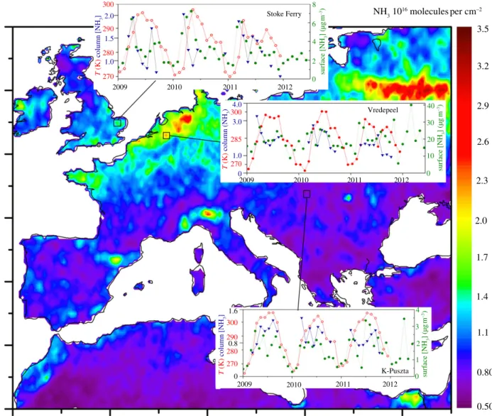
Such seasonal differences can also be seen from globally monitored satellite columns of NH3at 1212 km2resolution at nadir, through processing of retrievals from the infrared atmospheric sounding interferometer on the MetOp platform. This approach is based on the absorption spectra of NH3 in the infrared and depends on a strong thermal contrast between

rs

tb.r

oy

alsocietypublishing.org

Phil

Trans

R

Soc

B

368:

20130166

(7)

the ground and atmosphere, measuring NH3columns that are dominated by high concentrations in the lowest 1–2 km [37]. Retrievals are made twice a day, allowing extensive comparison with environmental and seasonal NH3dynamics.

An illustration of the satellite retrieval is shown in figure 5, which compares the mean NH3column over Europe with the seasonally varying NH3column at three sites where ground-based monitoring of NH3 concentrations is available. The map distinguishes areas of high agricultural NH3emissions in Brittany, E England, the Netherlands and NW Germany, Po Valley and Nile Delta, while showing high values across Belarus and SW Russia related to forest fires during 2010. The magnitude of the NH3 columns are also a function of spatial differences in atmospheric mixing that might explain why smaller values are seen in the west compared with the east of the UK. For Stoke Ferry, where NH3emissions are domi-nated by pig and poultry (see the electronic supplementary material, figure S1), both the ground-based and satellite data show spring peak NH3values, associated with land-spreading of manure. At Vredepeel, an area of intense pig and cattle farm-ing in the Netherlands, there is less seasonality in the NH3data, indicating a stronger contribution of controlled environment livestock housing. Lastly, at K-Puszta, a Hungarian site more distant from local sources, NH3levels are highest in summer and lowest in winter, reflecting the integration of different environmentally dependent sources.

The satellite approach requires a strong thermal contrast, limiting its capability in winter and cloudy conditions. How-ever, it allows the examination of spatial patterns and temporal trends with a global coverage that could never be achieved by ground-based air sampling. It thus provides an unprecedented opportunity to improve our understanding of the sources, management and climate controls on NH3, as further illustrated by seasonal NH3 patterns in different parts of the world. In the case of the Po Valley, Nile Delta, California and Pakistan, there is a strong seasonal cycle in NH3, with values ofQ10 of the column totals mostly in the

range 2–3. However, not all locations show such a tempera-ture-dependence, especially where management differences drive seasonality in NH3 emissions as seen in livestock dominated areas of Belgium and China (see the electronic supplementary material, figure S4). In order to derive the maxi-mum value from the satellite data, these, therefore, need to be interpreted using detailed atmospheric models, as a basis to disentangle the different driving factors.

5. Seabirds as a model system to assess

climate-dependence of global ammonia emissions

The preceding examples highlight the many factors controlling NH3emissions, including management effects. In the case of monitoring NH3 concentrations and atmospheric columns, an even larger number of meteorological factors affect observed values. For these reasons, there is a strong case to use model ecosystems to assess the climate-dependence of NH3exchange. At present, this can uniquely be demonstrated by the case of NH3emissions from seabird colonies, building on recent measurements and modelling [35,59].

Seabird colonies provide several advantages as a ‘model system’ to investigate the climate-dependence of NH3emissions: the birds follow a well-established annual breeding cycle little affected by human management; rates of Nrexcretion can be directly related to dietary energetics for well-characterized populations; and they typically form locally strong NH3sources in areas of low NH3background. Riddicket al.[35] estimated global NH3 emission from seabird colonies at 0.3 (0.1– 0.4) Tg yr21_{. Although this is a small fraction of total emissions,} it includes major point/island sources greater than 15 Gg NH3yr21, with sites distributed globally across a wide range of climates.

Colony-scale NH3flux measurements from seabird colo-nies were first reported by Blackall et al. [59] for Scottish islands, and these have been extended for contrasting climates 0.007

(a)

(b)

40 000

Gs

=

[NH

4

+)

s

/[H

+]

s

30 000

20 000

10 000

0 Nsubs T(–3)

Nsubs T(0) Nsubs T(+3) gamma T(0) gamma T(–3)

gamma T(+3) 0.006

0.005

0.004

0.003

0.002

1000

flux T(0) flux T(+3)

flux T(–3)

grass cut

fertilizer

NH

3

flux total (ng

m

–2

s

–1)

substrate nitrogen (kg

N per kg DM)

800

600

400

200

24 July 28 July 01 August 05 August 09 August 13 August 17 August 21 August 0

–200

Figure 4.

Effect of temperature scenarios (annual change of

þ3

8 C and

23

8 C) on (

a

) simulated nitrogen pools (foliar substrate N, and

G

s

) and (

b

) net NH

3

fluxes.

Simulations conducted using the PaSim model for managed grassland in Scotland following cutting and fertilization with ammonium nitrate.

rs

tb.r

oy

alsocietypublishing.org

Phil

Trans

R

Soc

B

368:

20130166

(8)

as illustrated in figure 6. In this graph, measured NH3 emis-sions have been normalized by calculated Nrexcretion rates to show the percentage of Nr that is volatilized (Pv). The measurements show a clear temperature-dependence across the globe, with Q103. For comparison, the dotted line is the estimate used by Blackallet al. [59] for global upscaling, whereas the solid line is the initial temperature-adjusted upscaling of Riddicket al.[35], following equation (3.3) (their scenario 2).

The importance of these measurements is emphasized by their use to verify a process-based model of NH3emissions, the GUANO model (see the electronic supplementary material, figure S5). The model is driven by excretal inputs according to bird diet, energetics and numbers combined with a water-bal-ance to estimate liquid-phase Nrconcentrations and run-off. Hydrolysis of uric acid to ammoniacal nitrogen is moisture-and temperature-dependent. By combining the modelled value of [NH4þ] with a guano pH of 8.5 and ground surface temperature, equation (3.3) allows estimation ofx(zo0). This is

then applied in equation (3.1) to calculate hourly NH3emission. Application of the GUANO model shows close agreement with measurements, the hourly NH3 fluxes responding to fluctuations in surface temperature, precipitation events and wind speed. The overall measured temperature-dependence is also reproduced by the GUANO model (figure 6),

including a difference between the two warmest sites, Michel-mas Cay and Ascension Island. This is explained by the latter being very dry, limiting rates of uric acid hydrolysis, and hence both measured and modelled NH3emission.

Based on the verification of the GUANO model with field measurements, the global seabird and excretion datasets [35] have been applied in the model for hourly simulation of 9000 colonies for 2010–2011 (figure 7). Ground temperature turns out to be the primary driver globally, withPvranging from 20 to 72 per cent for sites with annual mean temperature of 308C, whereas for sites with a mean temperature of 08C,Pv was 0 –18%. Variation between sites of similar temperatures is mainly attributable to differences in water availability, wind speed and nesting habitat (e.g. bare rock versus burrow breeders).

6. Climate-dependent assessment of ammonia

emissions, transport and deposition

The examples presented for terrestrial systems including grass-land, shrubgrass-land, forest and seabird colonies demonstrate the clear climatic dependence of NH3exchange processes. Agricul-tural systems are more complex, and include interactions with management (including alteration of management timing and

3.5 NH₃ 1016_molecules_{per cm}–2

300

285

270

T

(K)

column [NH

3

]

T

(K)

column (NH

3

)

2.0

4.0

3.0

1.0

0

300 290

270 280

T

(K)

column [NH

3

] 1.6

0.8

0

8

6

4

2

surf

ace [NH

3

] (µg

m

–3)

surf

ace [NH

3

] (µg

m

–3) 0

0 10 20 30 40

surf

ace [NH

3

] (µg

m

–3)

0 1 2 3 4

Stoke Ferry

Vredepeel

K-Puszta

2009 2010 2011 2012

2009 2010 2011 2012 1.5

1.0

290

280 270

3.2

2.9

2.6

2.3

2.0

1.7

1.4

1.1

0.80

0.50

Figure 5.

Satellite estimates of the NH

3

column (10

6

molecules cm

22

) and ground temperature, showing the mean for 2009, 2010 and 2011 (from the infrared

atmospheric sounding interferometer on the MetOp platform), as compared with ground-based measurements of atmospheric NH

3

concentrations at three

selected sites.

rs

tb.r

oy

alsocietypublishing.org

Phil

Trans

R

Soc

B

368:

20130166

(9)

systems), Nr type, animal housing and manure application method. In principle, however, many of the climatic inter-actions apply, and can be addressed using process-based models. The same is true for ocean–atmosphere NH3 exchange, which is bi-directional according to equation (3.1), withx(zo0) depending on variations in sea surface temperature,

[NH4þ] concentration, water pH and local NH3 air concen-trations. For example, future ocean acidification would tend to decrease sea-surface NH3emission. Of these factors, Johnson

et al.[60] found temperature to be of overriding importance in determining ocean NH3emissions, through its control ofx(zo0).

With this background, we return to the question of regional and global modelling of NH3emission, dispersion and depo-sition in CTMs. Section 2 showed that there are several limitations in current NH3emission inventories, such as infor-mation on activity data (numbers and location of animals, fertilizers, fires, etc.), average emission rates and data structure (distinction of source sectors). On a global scale, however, and given the target to assess climate change effects, by far the main limitation is that current architecture uses previously calculated emissions as input to CTMs. In reality, the same meteorology incorporated within a CTM to describe chemical 10

20 30 40 50 60 70 80 90 100

average temperature during measurements (°C)

percentage N volatilized as NH

3

(

Pv

,%)

whole island, Isle of May, Scotland (2004)

Michaelmas Cay, Australia

Signy Island, South Orkney

Big Mac, Bird Island

0 5 10 15 20 25 30 35

GUANO model measurements [59] measurements [35]

Bass Rock, Scotland (2004)

Ascension Island, South Atlantic

Puffin Colony, Isle of May, Scotland (2009)

Figure 6.

Measured percentage of excreted N

r

that is volatilized as NH

3

(

P

v

) as a function of mean temperature during field campaigns (dashed line:

P

v

(%)

¼

1.9354e

0.109

T

; R

2

¼

0.75), as compared with estimates from the GUANO model for a global selection of seabird colonies. The dotted line shows the value used in a

first bioeneregics (BE) model of Blackall

et al.

[59], while the solid line was applied in a temperature-adjusted bioenergetics (TABE) model, by Riddick

et al.

[35]

using equation (3.3). The bars on the measured points apply to colonies including burrow-nesting birds and indicate the estimated

P

v

if the colony were entirely

populated by bare-rock breeders.

180°W 160°W 140°W 120°W 100°W 80°W 60°W 40°W 20°W 0° 20°E 40°E 60°E 80°E 100°E 120°E 140°E 160°E

80°N

60°N

40°N

20°N

20°S

60°S

40°S

20°S

0°

average PV (%)

0–5

6–15

16–30

31–45

46–100

20° N

Pacific Ocean

Atlantic Ocean

Indian Ocean

Pacific Ocean

40° N 60° N

80° N

80°S

0°N

180°

180° 160°W 140°W 120°W 100°W 80°W 60°W 40°W 20°W 0° 20°E 40°E 60°E 80°E 100°E 120°E 140°E 160°E 180°

Figure 7.

Global application of the GUANO model illustrating the average percentage of excreted N that is volatilized as NH

3

. Excretion calculated based on colony

seabird energetics [35], combined with hourly meteorological estimates through 2010 – 2011.

rs

tb.r

oy

alsocietypublishing.org

Phil

Trans

R

Soc

B

368:

20130166

(10)

transport and transformation will have a major effect on short-and long-term control of NH3 emissions, deposition and bi-directional exchange. For example, on a warm sunny day, emissions from manure, fertilizers and plants will be at their maximum, whereas cuticular deposition of NH3will be at its minimum, with the same conditions promoting thermal con-vection in the atmospheric boundary layer, increasing the atmospheric transport distance.

To address the coupling of these processes requires a new paradigm for atmospheric NH3modelling. For this purpose, the long-term goal must be to replace the use of previously determined emission inventories with a suite of spatial activity databases and models that allow emissions to be cal-culated online as part of the running of the CTMs. Such an approach is already widely adopted for biogenic hydro-carbon emissions from vegetation [20]. In this way, both the environmental dependence of uni-directional NH3emissions and of bi-directional NH3 fluxes become incorporated into the overall model. In the case of the bi-directional part, online calculation is essential because of the feedback betweenx(z) and the direction/magnitude of the net flux.

An outline of the proposed modelling architecture is given in figure 8, with the key new elements highlighted in green. Instead of activity data and experimentally derived relationships being used directly to provide an ‘emissions inventory’, with sub-sequent (uni-directional) dry deposition, emissions are treated in two submodels: (i) uni-directional emissions from point sources such as manure storage facilities and animal housing (where x(zo0)x(z)) and (ii) bi-directional fluxes from area

sources (wherex(zo0) is less than or greater than x(z)), which

includes emissions or dry deposition according to prevailing conditions. The same meteorological data are thus used to

drive the emissions, chemistry transport and bi-directional exchange. With this structure, climatic differences between locations are incorporated, while climate change scenarios can be directly applied.

At the present time, many of the elements for a new archi-tecture are already available to build such a system at regional and global scales. Emission models such as those for animal houses and manure spreading [54,55] need to be linked to CTMs incorporating bi-directional exchange parametrizations. Simple process models, following the principles used in the GUANO model, should be further developed and their scope extended. While the most detailed dynamic model of bi-direc-tional canopy exchange [44] has many input uncertainties, the analysis of Neirynck & Ceulemans [53] suggests that a move from scheme 1 towards the simpler application of scheme 2 should be a feasible future target. These developments will require further information to parametrize G for ecosystem components, while upscaling models must include infor-mation on canopy and ground temperature, surface wetness and relative humidity and soil pH. While many of the necess-ary terms are available from meteorological models, a coupling with agricultural and ecosystem models becomes increasingly important for detailed simulation of the interactions. Challenges related to subgrid variability are addressed in the electronic supplementary material, S7.

Although not all these linkages have yet been made, signifi-cant progress in the temporal distribution of NH3 emissions according to agricultural activities has already been achieved, which can provide key input to the future developments [30,61,62]. For example, the US EPA Community Multiscale Air-Quality model includes coupling to an agro-ecosystem model to provide dynamic and meteorological-dependent

chemistry and transport module uni-directional

emission module (point)

meteorological model climate model

GCM/RCM

hourly emissions

bi-directional exchange module (area)

verification (and assimilation)

meteo data (T, ?, …) farm and other

statistics

climate drivers activity

data by sub-sector

land use and land cover

experimental emission relationships

earth observation and ground-based measurements

hourly air concs. and bi-directional fluxes

Figure 8.

Proposed modelling architecture for treating the climate-dependence of ammonia fluxes in regional and global atmospheric transport and chemistry

models. In this approach, static emission inventories are replaced by calculations depending on prevailing meteorology, while allowing for bi-directional exchange

with area sources/sinks, giving the basis to assess climate change scenarios including the consequences of climate feedbacks through altered NH

3

emissions. The

effect of altered air chemistry may also be fed back into the climate model.

rs

tb.r

oy

alsocietypublishing.org

Phil

Trans

R

Soc

B

368:

20130166

(11)

emissions from fertilizer application, using a two-layer bidirec-tional resistance model based on Nemitz et al. [15] that includes the effects of soil nitrification processes [18]. Similarly, Hamaoui-Lagelet al.[55] incorporated the VOLT’AIR model to simulate NH3emissions from fertilizer application in a regional-scale atmospheric model.

The consequences of such temporal interactions can be illustrated by the comparison of measured NH3 concentra-tion and simulaconcentra-tions of a Danish model [22] at a long-term monitoring site (Tange, electronic supplementary material, figure S6). In this case, the model has been used to provide the temporal disaggregation of previously calculated annual emissions. The challenge for the next stage must be to incor-porate the environmental drivers in process models for all major sources to quantify the dynamics on hourly, diurnal, seasonal and annual scales, and as a foundation to estimate the effects of long-term climate change.

7. Conclusions

This paper has shown how ammonia emissions and deposition are fundamentally dependent on environmental conditions. While temperature has been found to be the primary environ-mental driver, other key factors include interactions with canopy and soil wetness and with management practices for agricultural sources. For several systems, such as emission from manure spreading, fertilizers, seabird colonies and bidirectional exchange with vegetation, process models are already available that describe the key relationships.

A new paradigm for atmospheric modelling of NH3is pro-posed, where process models are incorporated with the relevant statistical data to simulate NH3emissions as part of atmospheric models. Seabird colonies have been used here to demonstrate the global application of such a process model, verified by measurements under different climates, where the fraction of available Nr volatilized as NH3 can increase by a factor of more than 20 between subpolar and tropical

conditions. Although a few CTMs have incorporated bidirec-tional exchange, work is required to parametrize models for different ecosystem types and climates, and to assess the con-sequences of different levels of model complexity, including the coupling with ecosystem and agronomic models.

The proposed developments provide the necessary foun-dation to assess how climate will affect NH3 emissions, dispersion and deposition. The practical implications are that inventory activities should focus increasingly on supplying the statistical activity data needed to drive the models (rather than only publishing static NH3emission estimates) and that national NH3emissions for any year can only be calculated with confidence once the meteorological data are available.

Based on the available measurements and models, it is poss-ible to indicate empirically the scale of the climate risk for NH3. Marine NH3emissions are expected to follow the thermodyn-amic response directly (equation (3.3)), whereas a reducedQ10 of 2 (1.5–3) may be applied for terrestrial volatilization sources. (For procedures, see the electronic supplementary material, section 8, figures S7, S8 and equations for use in scenario models.) Applying these responses to the 2008 global estimates of 65 (46–85) Tg N yr21_{for a 5}₈_{C global temperature increase} to 2100 would increase NH3emissions by approximately 42 per cent (28–67%) to 93 (64–125) Tg. If this is combined with a further 56 per cent (44–67%) increase in anthropogenic source activities [63,64], total NH3emissions would reach 132 (89–179) Tg by 2100. Considering these major anticipated increases, the limited progress in NH3 mitigation efforts to date, and the slow nature of behavioural change, stepping up efforts to control NH3 emission must be a key priority for future policy development.

Full acknowledgements, including from the European Commission, European Space Agency, US EPA, other national funding sources and individuals are listed in the electronic supplementary material. This paper is a contribution to the International Nitrogen Initiative (INI) and to the UNECE Task Force on Reactive Nitrogen (UNECE).

References

1. Erisman JW, Sutton MA, Galloway JN, Klimont Z, Winiwarter W. 2008 How a century of ammonia synthesis changed the world.Nat. Geosci.1, 636 – 639. (doi:10.1038/ngeo325)

2. Sutton MA, Erisman JW, Dentener F, Mo¨ller D. 2008 Ammonia in the environment: from ancient times to the present.Environ. Pollut.156, 583 – 604. (doi:10.1016/j.envpol.2008.03.013)

3. CEIP. 2012Overview of submissions under CLRTAP: 2012. Vienna, Austria: Centre for Emissions Inventories and Projections, Umweltbundesamt (www.ceip.at/overview-of-submissions-under-clrtap/2012-submissions/)

4. UNECE. 2012Draft decision on amending the text of and annexes II to IX to the Gothenburg protocol to abate acidification, eutrophication and ground-level

ozone and addition of new annexes X and XI.

Geneva, Switzerland: Executive Body for the Convention on Long-range Transboundary Air Pollution.

5. Pinder RW, Gilliland AB, Dennis RL. 2008 Environmental impact of atmospheric NH3emissions

under present and future conditions in the eastern United States.Geophys. Res. Letts.35, L12808. (doi:10.1029/2008GL033732)

6. Sutton MAet al. 2011 Summary for policy makers.

InThe European nitrogen assessment(eds MA

Sutton, CM Howard, JW Erisman, G Billen, A Bleeker, P Grennfelt, H van Grinsven, B Grizzetti), pp. xxiv – xxxiv. Cambridge, UK: Cambridge University Press.

7. Sutton MA, Oenema O, Erisman JW, Leip A, van Grinsven H, Winiwarter W. 2011 Too much of a good thing.Nature472, 159–161. (doi:10.1038/472159a) 8. Denmead OT, Freney JR, Simpson JR. 1976 A closed

ammonia cycle within a plant canopy.Soil Sci.

Biochem.8, 161 – 164.

(doi:10.1016/0038-0717(76)90083-3)

9. Farquhar GD, Firth PM, Wetselaar R, Wier B. 1980 On the gaseous exchange of ammonia between

leaves and the environment: determination of the ammonia compensation point.Plant Physiol.66, 710 – 714. (doi:10.1104/pp.66.4.710)

10. Sutton MA, Schjorring JK, Wyers GP. 1995 Plant atmosphere exchange of ammonia.Phil.

Trans. R. Soc. A351, 261 – 276. (doi:10.1098/rsta.

1995.0033)

11. Sutton MAet al. 2009 Dynamics of ammonia exchange with cut grassland: synthesis of results and conclusions of the GRAMINAE integrated experiment.Biogeosciences6, 2907 – 2934. (doi:10. 5194/bg-6-2907-2009)

12. Sutton MA, Reis S, Baker SMH (eds). 2009

Atmospheric ammonia: detecting emission changes

and environmental impacts, p. 464. Berlin, Germany:

Springer.

13. Schjoerring JK, Husted S, Mattsson M. 1998 Physiological parameters controlling plant – atmosphere ammonia exchange.Atmos. Environ.32, 491 – 498. (doi:10.1016/S1352-2310(97)00006-X)

rs

tb.r

oy

alsocietypublishing.org

Phil

Trans

R

Soc

B

368:

20130166

(12)

14. Hertel Oet al. 2011 Nitrogen processes in the atmosphere. InThe European nitrogen assessment

(eds MA Sutton, CM Howard, JW Erisman, G Billen, A Bleeker, P Grennfelt, H van Grinsven, B Grizzetti), Ch. 9, pp. 177 – 207. Cambridge, UK: Cambridge University Press.

15. Nemitz E, Milford C, Sutton MA. 2001 A two-layer canopy compensation point model for describing bi-directional biosphere/atmosphere exchange of ammonia.Q. J. Roy. Meteor. Soc.127, 815 – 833. (doi:10.1256/smsqj.57305)

16. Dentener FJ, Crutzen PJ. 1994 A three-dimensional model of the global ammonia cycle.J. Atmos.

Chem.19, 331 – 369. (doi:10.1007/BF00694492)

17. Wichink Kruit RJ, Schaap M, Sauter FJ, Van Zanten MC, van Pul WAJ. 2012 Modeling the distribution of ammonia across Europe including bi-directional surface-atmosphere exchange.Biogeosciences9, 5261 – 5277. (doi:10.5194/bg-9-5261-2012) 18. Bash JO, Cooter EJ, Dennis RL, Walker JT, Pleim JE.

2012 Evaluation of a regional air-quality model with bi-directional NH3exchange coupled to an

agro-ecosystem model.Biogeosciences10, 1635 – 1645. (doi:10.5194/bg-10-1635-2013)

19. Cape JN, van der Eerden LJ, Sheppard LJ, Leith ID, Sutton MA. 2009 Evidence for changing the critical level for ammonia.

Environ. Pollut.157, 1033 – 1037. (doi:10.1016/

j.envpol.2008.09.049)

20. Simpson Det al. 2011 Atmospheric transport and deposition of reactive nitrogen in Europe. InThe

European nitrogen assessment(eds MA Sutton,

CM Howard, JW Erisman, G Billen, A Bleeker, P Grennfelt, H van Grinsven, B Grizzetti), ch. 14, pp. 298 – 316. Cambridge, UK: Cambridge University Press.

21. Velthof VGL, van Bruggen C, Groenestein CM, de Haan BJ, Hoogeveen MW, Huijsmans JFM. 2012 A model for inventory of ammonia emissions from agriculture in the Netherlands.Atmos. Environ.46, 248 – 255. (doi:10.1016/j.atmosenv.2011.09.075) 22. Geels Cet al. 2012 A coupled model system

(DAMOS) improves the accuracy of simulated atmospheric ammonia levels over Denmark.

Biogeosciences9, 2625 – 2647.

(doi:10.5194/bg-9-2625-2012)

23. Dragosits U, Sutton MA, Place CJ, Bayley A. 1998 Modelling the spatial distribution of ammonia emissions in the UK.Environ. Pollut.102, 195 – 203. (doi:10.1016/S0269-7491(98)80033-X)

24. Webb J, Misselbrook TH. 2004 A mass-flow model of ammonia emissions from UK livestock production.

Atmos. Environ.38, 2163 – 2176. (doi:10.1016/j.

atmosenv.2004.01.023)

25. de Vries W, Leip A, Reinds GJ, Kros J, Lesschen JP, Bouwman AF. 2011 Comparison of land nitrogen budgets for European agriculture by various modeling approaches.Environ. Pollut.159, 3254 – 3268. (doi:10.1016/j.envpol.2011.03.038) 26. Bleeker Aet al. 2009 Linking ammonia emission

trends to measured concentrations and deposition of reduced nitrogen at different scales. In

Atmospheric ammonia: detecting emission changes

and environmental impacts(eds MA Sutton, S Reis,

SMH Baker), pp. 123 – 180. Berlin, Germany: Springer.

27. Misselbrook TH, Sutton MA, Scholefield D. 2004 A simple process-based model for estimating ammonia emissions from agricultural land after fertilizer applications.Soil Use Manag.20, 365 – 372. (doi:10.1079/SUM2004280) 28. Gross A, Boyd CE, Wood CW. 1999 Ammonia

volatilization from freshwater fish ponds.J. Environ.

Qual.28, 793 – 797. (doi:10.2134/jeq1999.

00472425002800030009x)

29. Sutton MA, Dragosits U, Tang YS, Fowler D. 2000 Ammonia emissions from non-agricultural sources in the UK.Atmos. Environ.34, 855 – 869. (doi:10. 1016/S1352-2310(99)00362-3)

30. Skjøth CAet al. 2011 Spatial and temporal variations in ammonia emissions: a freely accessible model code for Europe.Atmos. Chem. Phys.11, 5221 – 5236. (doi:10.5194/acp-11-5221-2011) 31. Bouwman AF, Lee DS, Asman WAH, Dentener FJ,

Van der Hoek KW, Olivier JGJ. 1997 A global high-resolution emission inventory for ammonia.Glob.

Biogeochem. Cycles11, 561 – 587. (doi:10.1029/

97GB02266)

32. Van Aardenne JA, Dentener FJ, Olivier JGJ, Klein Goldewijk CGM, Lelieveld J. 2001 A 1818

resolution data set of historical anthropogenic trace gas emissions for the period 1890 – 1990.Glob.

Biogeochem. Cycles15, 909 – 928. (doi:10.1029/

2000GB001265)

33. Beusen AHW, Bouwman AF, Heuberger PSC, van Drecht G, an Der Hoek KW. 2008 Bottom-up uncertainty estimates of global ammonia emissions from global agricultural production systems.Atmos.

Environ.42, 6067 – 6077. (doi:10.1016/j.atmosenv.

2008.03.044)

34. JRC/PBL. 2011 Emission database for global atmospheric research, EDGAR v. 4.2. See http:// edgar.jrc.ec.europa.eu/.

35. Riddick SN, Dragosits U, Blackall TD, Daunt F, Wanless S, Sutton MA. 2012 The global distribution of ammonia emissions from seabird colonies.

atmosenv.2012.02.052)

36. Andres RJ, Kasgnoc AD. 1998 A time-averaged inventory of subaerial volcanic sulfur emissions.

J. Geophys. Res.103, 25 251 – 25 261. (doi:10.1029/

98JD02091)

37. Clarisse L, Clerbaux C, Dentener F, Hurtmans D, Coheur PF. 2009 Global ammonia distribution derived from infrared satellite observations.Nat.

Geosci.2, 479 – 483. (doi:10.1038/ngeo551)

38. Bouwman AF, Boumans LJM, Batjes NH. 2002 Estimation of global NH3volatilization loss from

synthetic fertilizers and animal manure applied to arable lands and grasslands.Glob. Biogeochem.

Cycles16, 1024. (doi:10.1029/2000GB001389)

39. Flechard CR, Fowler D. 1998 Atmospheric ammonia at a moorland site. I. The meteorological control of ambient ammonia concentrations and the influence of local sources.Q. J. Roy. Meteor. Soc.124, 733 – 757. (doi:10.1002/qj.49712454705)

40. Fowler Det al. 2009 Atmospheric composition change: ecosystems: atmosphere interactions.

atmosenv.2009.07.068)

41. Nemitz E, Sutton MA. 2004 Gas-particle interactions above a Dutch heathland. III. Modelling the influence of the NH3–HNO3– NH4NO3equilibrium on

size-segregated particle fluxes.Atmos. Chem. Phys.4, 1025– 1045. (doi:10.5194/acp-4-1025-2004) 42. Loubet Bet al. 2009 Ammonia deposition near hot

spots: processes, models and monitoring methods. In

Atmospheric ammonia: detecting emission changes and

environmental impacts(eds MA Sutton, S Reis, SMH

Baker), pp. 205–267. Berlin, Germany: Springer. 43. Sutton MA, Burkhardt JK, Guerin D, Nemitz E,

Fowler D. 1998 Development of resistance models to describe measurements of bi-directional ammonia surface atmosphere exchange.Atmos.

Environ.32, 473 – 480.

(doi:10.1016/S1352-2310(97)00164-7)

44. Flechard C, Fowler D, Sutton MA, Cape JN. 1999 A dynamic chemical model of bi-directional ammonia exchange between semi-natural vegetation and the atmosphere.Q. J. Roy. Meteor. Soc.125, 2611 – 2641. (doi:10.1002/qj.49712555914) 45. Mattsson Met al. 2009 Temporal variability in

bioassays of the stomatal ammonia compensation point in relation to plant and soil nitrogen parameters in intensively managed grassland.

Biogeosciences6, 171 – 179.

(doi:10.5194/bg-6-171-2009)

46. Massad R-S, Nemitz E, Sutton MA. 2010 Review and parameterisation of bi-directional ammonia exchange between vegetation and the atmosphere.

Atmos. Chem. Phys.10, 10 359 – 10 386. (doi:10.

5194/acp-10-10359-2010)

47. Wichink Kruit RJ, van Pul WAJ, Sauter FJ, van den Broek M, Nemitz E, Sutton MA, Krol M, Holtslag AAM. 2010 Modeling the surface-atmosphere exchange of ammonia.Atmos.

Environ.44, 945 – 957. (doi:10.1016/j.atmosenv.

2009.11.049)

48. Riedo M, Milford C, Schmid M, Sutton MA. 2002 Coupling soil – plant – atmosphere exchange of ammonia with ecosystem functioning in grasslands.

Ecol. Model.158, 83 – 110.

(doi:10.1016/S0304-3800(02)00169-2)

49. Wu YH, Walker J, Schwede D, Peters-Lidard C, Dennis R, Robarge W. 2009 A new model of bi-directional ammonia exchange between the atmosphere and biosphere: ammonia stomatal compensation point.Agr. Forest Meteorol.149, 263 – 280. (doi:10.1016/j.agrformet.2008.08.012) 50. Massad R-S, Tuzet A, Loubet B, Perrier A, Cellier P.

2010 Model of stomatal ammonia compensation point (STAMP) in relation to the plant nitrogen and carbon metabolisms and environmental conditions.

Ecol. Model.221, 479 – 494. (doi:10.1016/j.ecol

model.2009.10.029)

51. Zhang L, Wright PL, Asman WAH. 2010 Bi-directional airsurface exchange of atmospheric ammonia: a review of measurements and a development of a big-leaf model for applications in

(13)

regional-scale air-quality models.J. Geophys. Res. 115, D20310. (doi:10.1029/2009JD013589) 52. Burkhardt Jet al. 2009 Modelling the dynamic

chemical interactions of atmospheric ammonia with leaf surface wetness in a managed grassland canopy.Biogeosciences6, 67–84. (doi:10.5194/bg-6-67-2009)

53. Neirynck J, Ceulemans R. 2008 Bidirectional ammonia exchange above a mixed coniferous forest.

Environ. Pollut.154, 424 – 438. (doi:10.1016/j.

envpol.2007.11.030)

54. Ge´nermont S, Cellier P. 1997 A mechanistic model for estimating ammonia volatilization from slurry applied to bare soil.Agr. Forest Meteorol.88, 145 – 167. (doi:10.1016/S0168-1923(97)00044-0) 55. Hamaoui-Laguel L, Meleux F, Beekmann M,

Bessagnet B, Ge´nermont S, Cellier P, Le´tinois L. 2012 Improving ammonia emissions in air quality modelling for France.Atmos. Environ. (doi:10.1016/ j.atmosenv.2012.08.002)

56. Søgaard HT, Sommer SG, Hutchings NJ, Huijsmans JFM, Bussink DW, Nicholson F. 2002 Ammonia volatilization from field-applied animal slurry—the ALFAM model.Atmos. Environ.36, 3309 – 3319. (doi:10.1016/S1352-2310(02)00300-X)

57. Nemitz E, Sutton MA, Wyers GP, Jongejan PAC. 2004 Gas – particle interactions above a Dutch heathland. I. Surface exchange fluxes of NH3, SO2, HNO3and

HCl.Atmos. Chem. Phys.4, 989 – 1005. (doi:10.

5194/acp-4-989-2004)

58. Hellsten S, Dragosits U, Place CJ, Misselbrook TH, Tang YS, Sutton MA. 2007 Modelling seasonal dynamics from temporal variation in agricultural practices in the UK ammonia emission inventory.Water Air Soil Pollut.

Focus7, 3–13. (doi:10.1007/s11267-006-9087-5)

59. Blackall TDet al. 2007 Ammonia emissions from seabird colonies.Geophys. Res. Lett.34, L10801. (doi:10.1029/2006GL028928)

60. Johnson MTet al. 2008 Field observations of the ocean – atmosphere exchange of ammonia:

fundamental importance of temperature as revealed by a comparison of high and low latitudes.Glob.

Biogeochem. Cycles22, GB1019. (doi:10.1029/

2007GB003039)

61. Gilliland AB, Appel KW, Pinder RW, Dennis RL. 2006 Seasonal NH3emissions for the continental United

States: inverse model estimation and evaluation.

atmonsenv.2005.12.066)

62. Skjoth CA, Geels C. 2013 The effect of climate and climate change on ammonia emissions in Europe.

Atmos.13, 117 – 128.

(doi:10.5194/acp-13-117-2013)

63. Fowler D, Pyle JA, Raven JA, Sutton MA 2013 The global nitrogen cycle in the twenty-first century: introduction.Phil. Trans. R. Soc. B368, 20130165. (doi:10.1098/rstb.2013.0165)

64. Fowler Det al. 2013 The global nitrogen cycle in the twenty-first century.Phil. Trans. R. Soc. B368, 20130164. (doi:10.1098/rstb.2013.0164)