UNIVERSIDAD POLITÉCNICA DE MADRID
ESCUELA TÉCNICA SUPERIOR
DE INGENIEROS DE TELECOMUNICACIÓN
TRABAJO FIN DE GRADO
TÍTULO:
Processing of ultra-wideband low-frequency signals, for
application in Foliage Penetration (FOPEN) Synthetic Aperture
Radar (SAR) systems
NOMBRE: Francisco Javier García Gómez
TUTOR: Mateo Burgos García
MIEMBROS DEL TRIBUNAL:
- PRESIDENTE: Félix Pérez Martínez
- VOCAL: Mateo Burgos García
- SECRETARIO: José Tomás González Partida
- SUPLENTE: José Ignacio Alonso Montes
FECHA DE LECTURA Y DEFENSA:
2
UNIVERSIDAD POLITÉCNICA DE MADRID
ESCUELA TÉCNICA SUPERIOR
DE INGENIEROS DE TELECOMUNICACIÓN
TRABAJO FIN DE GRADO
TÍTULO:
Processing of ultra-wideband low-frequency
signals, for application in Foliage Penetration
(FOPEN) Synthetic Aperture Radar (SAR) systems
NOMBRE: Francisco Javier García Gómez
3
Abstract
Foliage Penetration (FOPEN) radar systems were introduced in 1960, and have been constantly improved by several organizations since that time. The use of Synthetic Aperture Radar (SAR) approaches for this application has important advantages, due to the need for high resolution in two dimensions. The design of this type of systems, however, includes some complications that are not present in standard SAR systems.
FOPEN SAR systems need to operate with a low central frequency (VHF or UHF bands) in order to be able to penetrate the foliage. High bandwidth is also required to obtain high resolution. Due to the low central frequency, large integration angles are required during SAR image formation, and therefore the Range Migration Algorithm (RMA) is used. This project thesis identifies the three main complications that arise due to these requirements. First, a high fractional bandwidth makes narrowband propagation models no longer valid. Second, the VHF and UHF bands are used by many communications systems. The transmitted signal spectrum needs to be notched to avoid interfering them. Third, those communications systems cause Radio Frequency Interference (RFI) on the received signal.
The thesis carries out a thorough analysis of the three problems, their degrading effects and possible solutions to compensate them. The UWB model is applied to the SAR signal, and the degradation induced by it is derived. The result is tested through simulation of both a single pulse stretch processor and the complete RMA image formation. Both methods show that the degradation is negligible, and therefore the UWB propagation effect does not need compensation.
A technique is derived to design a notched transmitted signal. Then, its effect on the SAR image formation is evaluated analytically. It is shown that the stretch processor introduces a processing gain that reduces the degrading effects of the notches. The remaining degrading effect after processing gain is assessed through simulation, and an experimental graph of degradation as a function of percentage of nulled frequencies is obtained.
The RFI is characterized and its effect on the SAR processor is derived. Once again, a processing gain is found to be introduced by the receiver. As the RFI power can be much higher than that of the desired signal, an algorithm is proposed to remove the RFI from the received signal before RMA processing. This algorithm is a modification of the Chirp Least Squares Algorithm (CLSA) explained in [4], which adapts it to deramped signals. The algorithm is derived analytically and then its performance is evaluated through simulation, showing that it is effective in removing the RFI and reducing the degradation caused by both RFI and notching. Finally, conclusions are drawn as to the importance of each one of the problems in SAR system design.
4
Resumen
Los sistemas radar de penetración de la espesura (FOPEN) fueron introducidos en 1960, y han sido mejorados constantemente por varias organizaciones desde entonces. El uso de radares de apertura sintética (SAR) para esta aplicación tiene importantes ventajas, debido a la necesidad de alta resolución en dos dimensiones. Sin embargo, el diseño de este tipo de sistemas incluye algunas complicaciones que no están presentes en sistemas SAR estándar.
Los sistemas FOPEN SAR necesitan operar con frecuencia central baja (banda VHF o UHF) para poder atravesar la espesura. También se requiere un gran ancho de banda para obtener alta resolución. Debido a la baja frecuencia central, se necesitan ángulos de integración grandes durante el procesado SAR, y por tanto se utiliza el algoritmo RMA (Range Migration Algorithm). Este Trabajo Fin de Grado identifica las tres complicaciones principales que aparecen debido a estos requisitos. En primer lugar, el gran ancho de banda invalida los modelos de propagación de banda estrecha. En segundo lugar, las bandas VHF y UHF son utilizadas por muchos sistemas de comunicaciones. Es necesario eliminar ciertas bandas (notches) de la señal transmitida para evitar interferirlos. Por último, estos sistemas de comunicaciones causan interferencias de radio frecuencia (RFI) en la señal recibida.
El trabajo realiza un análisis exhaustivo de los tres problemas, sus efectos degradantes y posibles soluciones para compensarlos. El modelo de banda ultra-ancha (UWB) es aplicado a la señal SAR, y se calcula la degradación inducida. El resultado se comprueba mediante simulaciones, tanto de compresión de un solo pulso como de procesado RMA completo. Los dos métodos demuestran que la degradación es despreciable, y por tanto la propagación UWB no requiere compensación.
El trabajo deduce una técnica para aplicar notches a la señal transmitida. Se evalúa analíticamente el efecto de esto en la formación de imagen SAR, y se demuestra que la compresión de pulsos (deramp) introduce una ganancia de proceso que reduce el efecto degradante de los notches. La degradación residual después de la ganancia de proceso se evalúa mediante simulación, y se obtiene una gráfica experimental de degradación en función del porcentaje de frecuencias anuladas.
Por último, se caracteriza la RFI y se deduce su efecto en el procesado SAR. De nuevo se comprueba que el receptor introduce una ganancia de proceso. Como la potencia de las interferencias puede ser mucho mayor que la de la señal deseada, se propone un algoritmo para eliminar la RFI de la señal recibida antes del procesado RMA. Este algoritmo es una modificación del algoritmo CLSA (Chirp Least Squares Algorithm), explicado en [4], para adaptarlo a pulsos comprimidos mediante deramping. El algoritmo se presenta analíticamente y se evalúan sus prestaciones mediante simulación, mostrando su efectividad en la eliminación de RFI y en la reducción de la degradación causada por la RFI y por los
notches. Finalmente, se extraen conclusiones acerca de la importancia de cada uno de los problemas en el diseño de sistemas SAR.
5
Index
Chapter 1: Introduction and aim of the thesis ... 6
Chapter 2: Introduction to FOPEN SAR ... 7
2.1. Radar fundamentals ... 7
2.2. Pulse compression ... 8
2.3. SAR geometry ... 10
2.4. SAR image formation: the Range Migration Algorithm ... 11
2.5. SAR simulator design ... 14
2.5.1. Analog module ... 14
2.5.2. Digital module ... 14
2.5.3. NADC P-3 UWB SAR parameters used in the simulations ... 15
2.6. FOPEN SAR requirements ... 15
Chapter 3: Ultra-Wideband propagation model ... 16
3.1. Time-dependent delay ... 16
3.2. UWB model in stretch processing ... 16
3.3. Impact on SAR resolution ... 18
3.4. Results of UWB model on simulated data ... 19
3.4.1. Single pulse compression ... 19
3.4.2. Complete RMA image ... 21
Chapter 4: Notched transmit waveform implementation and effects ... 22
4.1. Notch requirements ... 22
4.2. Transmit waveform generation ... 22
4.3. Effect of stretch processing on notched signal ... 25
4.4. Results of transmit notching on simulated data ... 29
4.4.1. Single pulse compression ... 29
4.4.2. Complete RMA image ... 30
Chapter 5: Radio Frequency Interference removal ... 33
5.1. RFI characteristics ... 33
5.2. Effect of stretch processing on RFI ... 34
5.3. Elimination of RFI: Chirp Least Squares Algorithm applied to a deramped signal ... 38
5.3.1. Target signal clipping ... 39
5.3.2. Standard RFI estimation ... 39
5.3.3. Commercial FM estimation ... 42
5.4. Results of CLSA on simulated data ... 43
5.4.1. Single pulse compression ... 44
5.4.2. Complete RMA image ... 45
Chapter 6: Conclusions and results ... 49
6
Chapter 1:
Introduction and aim of the thesis
Foliage Penetration (FOPEN) radar systems are being developed since the 1960s, when a large UHF antenna was used with this purpose for the first time, as part of the Camp Sentinel program. Since that time, several organizations have been researching and developing these systems. For the last 15 years, Synthetic Aperture Radar (SAR) [2] systems have been the main option for FOPEN operation. This is due to the high resolution requirement in both the range and cross-range dimensions, which makes synthetic aperture an attractive solution. The design of this type of radars includes certain additional complications with respect to that of conventional systems, and the detection of small, slow moving vehicles remains a challenge as of today.
In order for the signal to be able to penetrate the foliage, it is necessary to use low-frequency bands (UHF or VHF), so that the wavelength of the SAR signal is greater than the foliage dimensions. Due to the small size of the targets intended for detection, a high spatial resolution must be guaranteed. This requires the use of large bandwidths, which, combined with the low central frequency, invalidate narrow-band approximations. The Ultra-Wideband (UWB) propagation model needs to be applied, which may introduce degradation on SAR processing. The need for good spatial resolution also makes the use of SAR systems with high azimuth integration time an attractive solution. This requires high capacity processors.
In addition, UHF and VHF bands are populated with numerous communications systems. This introduces two additional complications on the design of FOPEN SAR systems. First, the transmitted signal spectrum needs to be notched to avoid interfering the communications systems, which would violate the regulations. An effective technique needs to be implemented to generate a notched chirp signal for transmission. Second, the communications systems introduce Radio Frequency Interference (RFI) on the received signal. Both the notches and the RFI can have a degrading effect on SAR image formation.
FOPEN SAR systems play a very important role in both military and earth resource measurement applications, but the design of these systems is still evolving and there is room for future research. With this in mind, the aim of this thesis is to determine the additional considerations that need to be taken in order to design a functional FOPEN SAR system, as opposed to a standard SAR system. To achieve this, the three problems described above will be analyzed: UWB propagation, transmit signal notching, and presence of RFI. The UWB model will be applied to the SAR signal. A technique for effective notching of the transmit signal will be explained, and its effects on the operation of the receiver will be derived. The RFI will be characterized, and the degradation it causes will also be calculated. All the results will be verified through simulation of both a single pulse stretch processor and complete RMA image formation.
After each one of the effects has been analyzed and simulated, an assessment of the importance of the degradation it can cause on a SAR system will be done. In the cases where it turns out to be too harmful to the system, a digital processing algorithm to mitigate the effect will be proposed and analyzed. The performance of the algorithm will be evaluated through further simulation.
7
Chapter 2:
Introduction to FOPEN SAR
In this chapter, the fundamentals of Synthetic Aperture Radar (SAR) systems will be presented, as well as the image formation algorithm that will be used in the whole project thesis: the Range Migration Algorithm (RMA). The aim of this introduction chapter is to outline the fundamentals of the SAR technique and to settle the notation that will be used throughout the rest of the thesis. Therefore, only the basic concepts and final results will be shown, and references will be given for the derivation of those results.
2.1.
Radar fundamentals
The radar systems that will be analyzed in this project thesis are pulsed systems. They transmit a time-limited signal (or pulse) with a duration T, and wait to receive its echoes. Then they repeat this process periodically. The period of this repetition is the Pulse Repetition Interval (PRI), and its inverse is the Pulse Repetition Frequency (PRF). Figure 1 shows the transmitted signal and these parameters.
Figure 2.1 Pulsed radar transmitted signal
The reflection of this signal from a single point scatterer at a distance is received with a delay equal to the time it takes an electromagnetic wave (travelling at the speed of light c) to cover twice that distance:
(2.1)
To avoid ambiguities, the received signal must lie within the receive window of its corresponding transmitted signal. This places an upper and lower limit on the distance to the scatterer, which ideally (zero switching time from transmit to receive) are:
(2.2)
The received power from a target can be calculated from the radar equation [1]:
(2.3)
where,
8
= peak received power
= transmitter antenna equivalent area = receiver antenna equivalent area
, radar cross section (RCS) of the target [1]
= radar wavelength =additional losses
2.2.
Pulse compression
The distance resolution that can be obtained with a rectangular pulse is:
(2.4)
This means that a smaller pulse duration will improve resolution. However, smaller duration also means lower transmitted energy, which reduces SNR. To overcome this tradeoff, many radar systems use a technique called pulse compression [2].
Pulse compression aims to transmit a long pulse (high SNR) that can be processed after reception to obtain high resolution. The initial idea was to transmit a linear FM (LFM) signal, whose expression in baseband is:
(2.5)
where is the linear FM rate (Hz/s) and is the rectangle function, with value 1 in
and 0 elsewhere. Figure 2.2 outlines the waveform of the actual (non-baseband) transmitted chirp pulse.
Figure 2.2 Outline of a modulated chirp signal
The instantaneous frequency of this signal is a linear frequency ramp:
9
The Fourier transform of is derived in [2] by applying the Principle of Stationary Phase
(POSP). The result, ignoring a multiplicative constant which will be calculated in Chapter 3, is:
(2.7)
This signal has a bandwidth of:
(2.8)
The signal modulates a carrier with frequency , which is transmitted, reflected by a scatterer and received with a delay :
(2.9)
where is a complex constant that depends on the reflectivity and the radar equation and which is irrelevant to our purpose. At this point, there are two ways to process the signal to obtain high resolution: matched filtering [2] and stretch processing [3]. Matched filtering achieves optimal results, but requires a digital processor that can process the whole bandwidth of the signal. Stretch processing is a good approximation when certain conditions are met, and requires a much lower digital bandwidth. Due to the high bandwidth of the signals in FOPEN SAR, stretch processing will be used in this project thesis.
Figure 2.3 Stretch processor block diagram
Figure 2.3 depicts the block diagram of the stretch processor. Stretch processing, also known as
deramping, can only compress targets whose delays are within a small time interval, with center and length . The frequency-time diagrams of two targets at both ends of this receive interval are shown in Figure 2.2. Stretch processing consists of mixing (multiplying in the time domain) the received signal
with a (complex conjugate) replica of the transmitted signal.
(2.10)
where . Mixing two frequency ramps with the same slope results in a tone:
10
where and (the time origin is now the center of the receive window). This signal is a tone with frequency , proportional to the target relative delay. A change of variable
, followed by an inverse Fourier transform (IFFT), yields:
(2.12)
which is a sinc signal, centered at the position of the target and with a distance resolution (3-dB width) of:
(2.13)
This means that, if is chosen such that (time-bandwidth product TBP>1), pulse compression achieves better resolution for a given transmitted pulse duration . Side lobe reduction can be achieved with a slight loss of resolution by applying a smoothing window to in (2.12).
The ADC sampling occurs when the signal is of the form given in Equation (2.11). As
, the bandwidth of this complex signal is , which is the required sampling frequency, instead of the required for matched filter systems. Deramp systems are designed so that , and therefore require much lower digital processor capability than the matched filter approach. A low pass filter (gray shade in the frequency-time diagram in Figure 2.3) is applied before sampling to avoid aliasing from interfering signals.
2.3.
SAR geometry
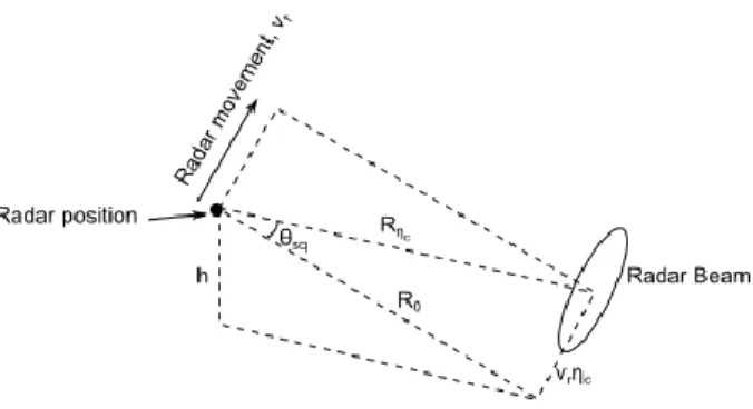
Figure 2.4 SAR geometry
Synthetic Aperture Radar (SAR) consists of a moving radar platform (airplane or satellite) that explores the ground and obtains high resolution in the direction of movement (azimuth) by integrating the received signal over several pulses, and applying an imaging algorithm to create an equivalent synthetic antenna aperture, with a length equal to the distance covered during those pulses. Resolution in the direction of the beam (slantrange) is achieved through pulse compression.
11
: Azimuth time from closest approach to scene center
: Slant range of closest approach
: Slant range of scene center : Radar velocity
All the derivations are done with the approximation that both the radar and the targets are static for the duration of the pulse (in Chapter 3 we will assess the effect of this approximation). With this assumption, two time variables are defined: range (fast) time, , the time with respect to which each single transmitted pulse is defined, and azimuth (slow) time, η, the absolute time that defines when the pulses are sent. With these definitions, the range (hyperbolic) equation of a SAR system is:
(2.14)
which gives the distance to the scatterer as a function of azimuth time.
The received signal from a point target is then [2]:
(2.15)
where is an irrelevant complex multiplicative constant, is the window applied to the transmitted pulse (replaces the function in (2.5)), and is the antenna beam pattern (which effectively applies a window to the signal in the azimuth time dimension).
It can be shown that the resulting received signal in the azimuth time dimension is also a linear FM (chirp) signal. The equivalent azimuth chirp rate is:
(2.16)
The equivalent azimuth signal bandwidth is:
(2.17)
where is the antenna azimuth beamwidth. The PRF of the radar should be higher than this to avoid aliasing. Additionally, Equation (2.2) imposes an upper limit on PRF, which should therefore be chosen between these two bounds.
2.4.
SAR image formation: the Range Migration Algorithm
12
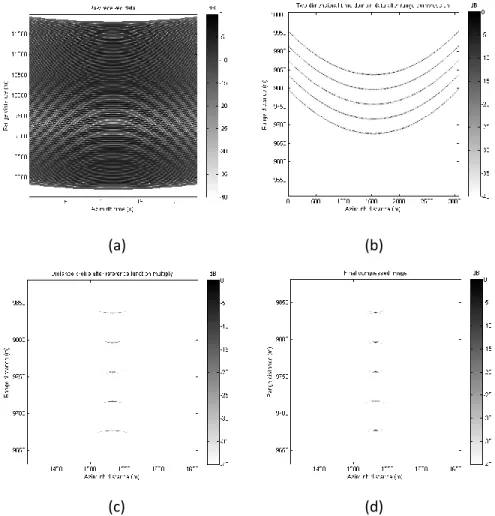
processing along the range dimension, normally referred to as range compression. Figure 2.5 (b) shows how the data from the 5 scatterers look like after range compression.
Figure 2.5 SAR data from five point scatterers: (a) raw data, (b) after range compression, (c) after reference function multiply, (d) final compressed image. Note that (c) and (d) have been zoomed in for visibility purposes.
As the radar platform moves, the distance to the target varies according to (2.14), resulting in a shape similar to a parabola for . This is called range cell migration (RCM). The purpose of SAR
imaging algorithms is to correct this migration and equivalently transform every target's signature to a straight line, and then compress it in the azimuth direction using matched filtering [2, 3].
Each SAR imaging algorithm has its advantages and disadvantages that make it best suited for certain applications. FOPEN SAR requires a long integration time, which results in high RCM and high computational load. The Range Migration Algorithm (RMA) operates in the two-dimensional frequency domain, can correct high RCM, and is not too demanding as far as computational capability is concerned. Its main disadvantage is that it cannot accommodate variations of equivalent radar velocity with range or long swath width (range time extent). Both of these problems are negligible in the case of an airborne platform, so the RMA is the most appropriate option for FOPEN SAR.
(a) (b)
13
Figure 2.6 RMA block diagram
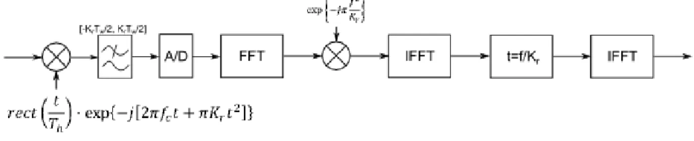
Figure 2.6 shows the block diagram of the RMA. The raw data in Figure 2.6 is obtained directly from the deramp mixer (without change of variable or IFFT), and has the form of Equation (2.11) for each azimuth column. The phase of the signal is:
(2.18)
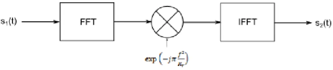
The first term is a tone at with a frequency proportional to the distance to the target; the second term contains information on the phase history of the target. But the third term is a residual quadratic phase term called residual video phase (RVP) that introduces errors when integration time is long, as is the case for FOPEN SAR systems. The range deskew step [3] eliminates this term by applying a frequency-dependant delay to the signal, which is equivalent to multiplying its FFT by , as
shown in Figure 2.7.
Figure 2.7 Range deskew block diagram
After RVP removal, the change of variable is performed. The signal is now in the range
frequency, azimuth time domain. An FFT in the azimuth dimension converts it to the 2-D frequency domain. The signal phase is now [2]:
(2.19)
The signal is then multiplied in this domain by the reference function:
(2.20)
yielding a signal with phase:
(2.21)
where is the reference range, usually the range at the center of the scene. Figure 2.5 (c)
14
respect to ) phase when , meaning targets at range are now correctly focused. RCM
remains for targets at other ranges, which is called differential RCM and is eliminated by the Stolt interpolation step. Note that Figure 2.5 (c) and (d) have been zoomed in for visibility purposes.
The Stolt interpolation consists of applying a change of variable to the signal in (2.21) that transforms it to a linear phase ramp for each target. The change to apply is:
(2.22)
This change is applied by using an interpolator, usually a sinc interpolator [2], to calculate the signal value at the new frequency points . After Stolt interpolation, the signal phase becomes:
(2.23)
A two-dimensional IFFT completes the process, resulting in a compressed target image:
(2.24)
where and are the inverse Fourier transform of the range and azimuth windows
respectively, which are sinc-like functions. The target is therefore registered to and , which is the position of closest approach. Figure 2.5 (d) shows the final compressed targets.
2.5.
SAR simulator design
A SAR simulator has been developed in MATLAB, which will be used to test all the effects and proposed solutions throughout the project thesis. The simulator has two main components: the analog module and the digital module.
2.5.1.Analog module
The analog module simulates the propagation of the SAR pulses. The propagation of a pulse sent
every
is simulated using (2.9), with the application of the Radar Equation (2.3) to calculate the
multiplicative constant . The simulator supports multiple scatterers, and simulates both the motion of the radar platform at a velocity of along the Y axis and a sinc-squared antenna radiation diagram. Additionally, simulation of wideband propagation (Chapter 3), notched transmission (Chapter 4) and narrowband radio frequency interference (RFI, Chapter 5) is also performed in this module.
The reflected signals from each scatterer are summed together to calculate the complete response for the current pulse. Then, the deramp mixer of (2.10) is applied (along with a Kaiser window of
for side lobe reduction), obtaining a signal of the form of (2.11). The sampling frequency of the analog module simulation is the maximum bandwidth of the received signal: .
2.5.2.Digital module
Once a signal of the form of (2.11) is obtained, a (complex) low-pass filter of bandwidth
15
vertical axis is range time. The five steps of RMA are applied to the raw data matrix as shown in Figure 2.6, and a final compressed image is obtained. The RFI removal step will be added after the range deskew step in Chapter 5.
All the SAR images shown in this project thesis are obtained with this simulator, including the ones in Figure 2.5.
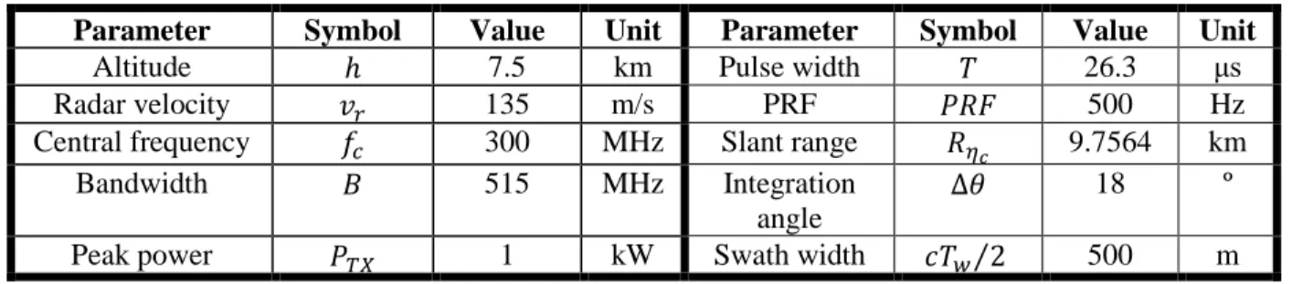
2.5.3.NADC P-3 UWB SAR parameters used in the simulations
All the simulations in this thesis use the parameters of a real system: NADC P-3 UWB SAR [4]. Table 2.1 lists these parameters. The only parameter that is different from the P-3 system is the swath width, which was lowered from 929 to 500 m due to computational limitations. This difference has no relevance to the purpose of this thesis.
Table 2.1 NADC P-3 UWB SAR parameters used in the simulations
Parameter Symbol Value Unit Parameter Symbol Value Unit
Altitude 7.5 km Pulse width 26.3 μs
Radar velocity 135 m/s PRF 500 Hz
Central frequency 300 MHz Slant range 9.7564 km Bandwidth 515 MHz Integration
angle
18 º
Peak power 1 kW Swath width 500 m
2.6.
FOPEN SAR requirements
This section presents the specific requirements for FOPEN SAR systems and the problems they create, whose characterization and solution are the main purpose of this project thesis. Chapters 3, 4, and 5 will treat each one of these problems separately, assess their effects, propose a solution and test it. Chapter 6 will summarize the main results of the three analyses.
In order for the transmitted signal to be able to penetrate the foliage, a low center frequency (long wavelength) is required (VHF or UHF). The targets intended for detection are usually small vehicles, which means a high resolution is needed. For the azimuth dimension, this means a high integration angle, which is addressed by the use of RMA. For the range dimension, it means a high bandwidth, which, combined with the low central frequency, invalidates the narrow-band propagation models. Ultra-wideband (UWB) propagation models have to be applied, which may degrade the algorithm results. Chapter 3 will analyze the implications of applying these models and add them to the simulations.
16
Chapter 3:
Ultra-Wideband propagation model
The first one of the potentially degrading effects to FOPEN SAR that will be analyzed in this project thesis is the Ultra-Wideband (UWB) propagation model. Due to the high bandwidth and low central frequency characteristic to FOPEN SAR systems, the fractional bandwidth (ratio of bandwidth to central frequency) is usually much higher than the Ultra-Wideband threshold (25%), typically being around 100% and sometimes even reaching 170-180% [4]. The P-3 system that will be simulated has a fractional bandwidth of 171.67%.
In this chapter, a detailed explanation of the UWB propagation model will be given, and then it will be applied to the FOPEN SAR equations. The degrading effect of UWB propagation will then be assessed. Finally, simulation data will be shown to verify the results.
3.1.
Time-dependent delay
In order to characterize the propagation of a wideband radar signal coming from a moving platform, time-dependant delay must be taken into consideration [5]. The different parts of the signal in the time domain cannot be considered to have the same propagation delay, as they were generated from different positions of the platform. As explained in [6], the Doppler frequency shift approximation is not valid either when ultra-wideband signals are concerned. The complete time-dependant delay model must be applied:
(3.1)
where is the distance from the platform to the scatterer as a function of time, and is the time-dependant delay. The time origin is taken to be the center of the transmitted pulse. This equation basically states that the delay at a time instant is twice the time it takes the signal to cover the distance between the platform and the scatterer at a time instant corresponding to half that delay.
To simplify the calculations, a time instant is defined, which is the instant at which the center of the transmitted signal (the part of the signal that was transmitted at ) is received:
(3.2)
As the received signal will be spread around , a Taylor expansion of around this point will be used for the analysis. The first and second derivative of at can be easily calculated from (3.1) and (3.2). The result is:
(3.3)
where and are respectively the first and second derivatives of evaluated at .
3.2.
UWB model in stretch processing
17
(3.4)
Applying the time-dependant delay of (3.1) to (3.4):
(3.5)
From (3.3):
(3.6)
where, to make the following expressions clearer, the new variables
, , and
have been used. Substituting (3.6) into (3.5) yields:
(3.7)
where the terms of order higher than 2 are negligible and have been removed. The receiver will be centered at . Let be the position of the center of the target's return with respect to the receiver's time origin (this is the same notation that was used in (2.10)-(2.12)). The receiver is a coherent I-Q receiver with stretch processing, as shown in Figure 3.1.
Figure 3.1 Deramp I-Q receiver
The demodulated and deramped signal is then:
(3.8)
where, after substituting back the values of and ,
18 (3.12)
Comparing this equation with (2.11), it can be seen that the tone with frequency has a
Doppler error given by
, and there is an additional quadratic term
.
The residual video phase (RVP) is the same as in the narrowband case (the minus sign in the RVP is due to the time origin being at the target's center in this analysis instead of being at the center of the receive window. Substituting would give the positive RVP).
The conversion of these errors to range units can be done easily, knowing that .
Assuming , which always happens in airborne SAR platforms, the range misregistration due to the Doppler error is:
(3.13)
The quadratic phase error (QPE, phase deviation at the ends of the pulse) introduced by the quadratic term is:
(3.14)
The distance to the target in an airborne platform, assuming that the platform moves along the Y axis, has the form:
(3.15)
where are constants. The values of and are the first and second derivative of
evaluated at :
(3.16)
(3.17)
where is the coordinate of the platform at .
3.3.
Impact on SAR resolution
The maximum value that can take is approximately the sine of half the integration angle, no more than 1 in any case. One way to evaluate the importance of the Doppler misregistration is by comparing it with the range resolution:
19
In the case of FOPEN SAR platforms, is in the tens or hundreds of m/s, and is in the units or tenths of a meter. This means that, for pulse widths under 100 μs, Doppler misregistration is much lower than range resolution and therefore does not cause any degradation. In the case of the P-3, the value
of is at the ends of the integration angle, making the Doppler misregistration negligible.
The quadratic error term introduces a quadratic phase error that degrades the range resolution. The QPE for the FOPEN SAR case is, from (3.14), (3.16) and (3.17):
(3.19)
In an FOPEN SAR system, and are comparable to each other. At the center of the
integration angle, the first term of (3.18) is 0, and the QPE becomes
. In the same way as for the
Doppler misregistration, we can assume that , and certainly that , which makes the
QPE at the center of the integration period insignificant ( in the case of the P-3).
At the edges of the integration angle, (as is the distance covered by the platform during the transmission of one pulse and is the distance it covers in half the integration period). This
means that the first term of (3.18) is dominant, and the QPE at the edges of the integration is .For radar velocities in the hundreds of meters per second, the time-bandwidth product (TBP) required for this to be important (more than 0.1π, as explained in [2]) is greater than , if the integration angle is 90º. Such high values are not used, and the quadratic error introduced by UWB propagation is also negligible in most systems. For the P-3, the resulting QPE at the ends of the integration angle is .
3.4.
Results of UWB model on simulated data
In the previous section, it has been shown that both the misregistration and the resolution loss due to the UWB model are negligible for typical FOPEN SAR systems. To verify this result, simulations with the P-3's parameters (Table 2.1) have been carried out. The following subsections will present the results obtained by the simulations.
All the simulations and algorithm tests in this project thesis will be done in two parts. First, the degradation effect or algorithm performance will be tested on the stretch processing of a single pulse. The degradation can more easily be seen or evaluated on an one-dimensional signal. Then, the effect or algorithm will be applied to a the complete RMA for SAR image formation. This second simulation gives a less clear view of the degradation but allows verification that the image formation still works properly under the new conditions, which is the ultimate purpose of the thesis.
3.4.1.Single pulse compression
20
Impulse Response Width (IRW): distance in the horizontal axis between the two -3 dB- points around the maximum. In this thesis, IRWs are given in range units.
Side Lobe Level (SLL): ratio in dB of the highest side lobe's maximum to the absolute maximum.
Integrated Side Lobe Ratio (ISLR): ratio in dB of energy in the side lobes to energy in the main lobe. This is the most representative parameter, which gives the clearest idea as to how much energy remains defocused after pulse compression.
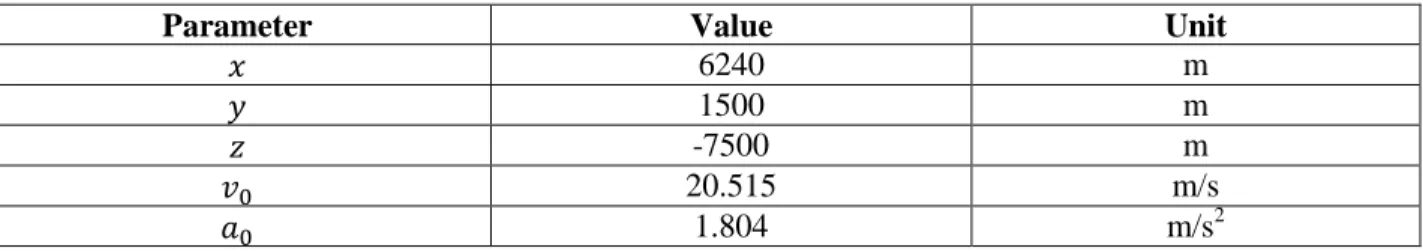
In order to test the UWB model on a single pulse compression process, Equations (3.3), (3.16) and (3.17) have been added to this part of the developed simulator. The parameters used are those in Table 2.1. A single target has been simulated at the edge of the integration angle. The distance coordinates of the target to the platform (which moves along the Y axis), as well as the corresponding relative movement parameters and , obtained from (3.16) and (3.17), can be found in Table 3.1.
Table 3.1 Target parameters for UWB single pulse simulation
Parameter Value Unit
6240 m
1500 m
-7500 m
20.515 m/s
1.804 m/s2
The simulation has been done with the UWB model and with the narrowband approximation, to allow comparison. Figure 3.2 shows the simulation results.
Figure 3.2 Single pulse UWB model simulation
21
attributed to quantization issues due to the use of the lowest possible sampling frequency allowed by the Sampling Theorem.
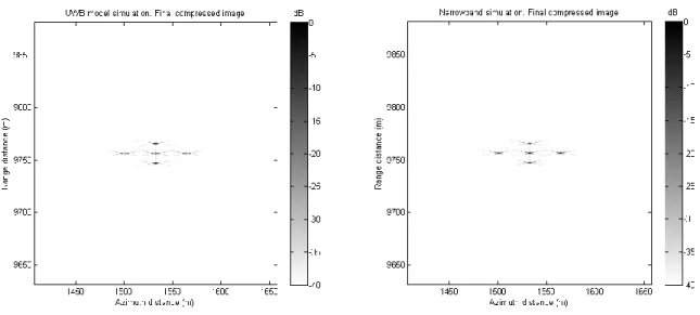
3.4.2.Complete RMA image
The UWB model was next applied to the complete RMA image formation algorithm, to see if UWB propagation had any effect on azimuth integration. Figure 3.3 shows an image with a single target with and without UWB propagation.
Figure 3.3 Complete image UWB simulation, single target: (a) UWB simulation, (b) Narrowband simulation
The differences between the two models are once again negligible. It can be safely concluded that the UWB propagation has no degradation effects on the SAR processing chain. Finally, Figure 3.4 shows another comparative simulation with 5 targets.
22
Chapter 4:
Notched transmit waveform implementation and effects
The second issue that must be taken into consideration for the design of FOPEN SAR systems is the potential interference to communications systems operating in the SAR frequency band. The use of a high bandwidth in the VHF or UHF bands implies that there are a considerable amount of other systems that may be interfered. Regulations against interference by several organizations must not be violated in order to obtain a license to operate the SAR platform. The high power of radar signals compared to communications signals complicates the solution to the problem, requiring the application of precise notches on the transmitted chirp signal. This chapter will outline the steps needed to decide where notches should be applied, present and analyze a technique to apply the notches, and evaluate the impact of the notches on the final resolution of the SAR image with the use of simulations.
4.1.
Notch requirements
Several organizations regulate the use of the spectrum and the interference limits. When designing a FOPEN SAR system, regulations from international, regional and national organizations must be taken into account. The steps to be taken to design a system that fulfills all the requirements are [4]:
Identify the geographic region of operation, and which organizations regulate the use of the frequency spectrum in that region. The International Telecommunication Union Radio Regulations (ITU-RR) [7] must always be taken into account. Some regions have additional regulations by regional organizations, such as the European Communications Committee (ECC) [8]. Finally, country-specific regulations must also be considered, which can usually be found in the respective country's regulation organism website.
Determine the locations of all the receivers that could be interfered by the SAR system.
Apply the most suitable propagation model to assess the interfering power.
If the interfering power exceeds any of the limitsimposed by the regulations, apply a notch on the transmitted signal.
This is a thorough analysis and requires careful analysis. Several propagation models exist, which are best suited for different scenarios. As this is an evaluation of interference from an airborne platform, the free space propagation model can be safely used as a worst-case scenario for a quick analysis. The effect of obstacles can be assessed by using Rec. P-526 of the ITU-R [9], or any other suitable model. In any case, the evaluation of the interfering power itself is outside the purpose of this thesis.
4.2.
Transmit waveform generation
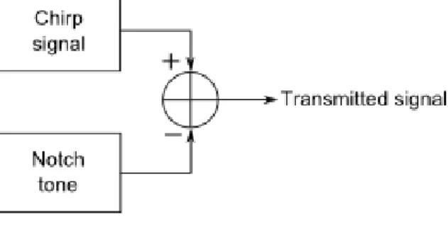
There are several ways to implement the narrow frequency notches on the transmitted waveform. The two most important ones are Frequency Jump Burst (FJB), which consists of transmitting each of the signal frequency chunks consecutively in time, with rapid frequency hops, and Notched Linear FM (NLFM), which consists of subtracting tones from the transmit waveform. This thesis will focus on the NLFM approach; further information on FJB can be found in [4].
Figure 4.1 shows the basic representation of the notch transmitter. For each one of the required notch frequencies, a tone is generated and subtracted from the chirp signal.
23
of the chirp signal at each frequency. The Principle of Stationary Phase (POSP) needs to be applied for this: this section will derive the required amplitude and phase.
Figure 4.1 Notch transmitter block diagram
The derivation will be done in the baseband domain, and then the result will be converted to a real signal. Suppose a standard chirp transmit signal as given by:
(4.1)
and a required notch depth of at frequency . The first step is to calculate
the Fourier transform of , and evaluate it at :
(4.2)
The Principle of Stationary Phase [2] states that an integral of the form:
(4.3)
where
(4.4)
can be approximately solved if the phase is stationary (its derivative is 0) for some value of the time variable. In this case, the phase of the integrand has a stationary point that depends on . Then, a time-frequency relationship can be obtained by forcing , where the prime denotes the first derivative with respect to . The approximate result of the integral is:
(4.5)
where:
(4.6)
24
(4.8)
and the sign of is given by the sign of , the second derivative of with respect to
evaluated at . The constant is usually ignored in most analyses, however, it is needed to know the amplitude and phase of the notch tone to subtract.
The POSP will now be applied to derive the solution of the integral in (4.2). The stationary point is , obtained from . Making yields:
(4.9)
which, substituted in (4.5), (4.6), (4.7), and (4.8) yields:
(4.10)
The notch tone has the form:
(4.11)
whose Fourier transform is:
(4.12)
This signal is subtracted from . To introduce a notch of depth , the following equation must hold:
(4.13)
where is the notch attenuation at its center frequency, expressed as a voltage gain.
Substituting the values of the signals, the required amplitude can be calculated:
(4.14)
where the sign of is once again the sign of . This signal can be easily transformed to the real-valued modulated signal. If the chirp signal has the form:
(4.15)
25
(4.16)
where:
(4.17)
(4.18)
and the sign of is the same as the sign of .
With (4.14) or (4.16), the notch waveform can be implemented in either the digital or the analog domain. Figure 4.2 shows the three signals , , and the transmitted signal
for a single notch of depth and frequency . This figure only
aims to give a clear view of the signals in the process, therefore, the pulse duration has been reduced to 0.5 μs to make the cycles visible.
Figure 4.2 Signals in the NLFM process
4.3.
Effect of stretch processing on notched signal
26
(4.19)
where, from (2.9),
(4.20)
and, from (4.16),
(4.21)
where and are given by (4.17) and (4.18) respectively. The time origin has been
chosen to be the center of the receive window ( ), and is the delay from the center of the receive window to the center of the target's returned signal. The complex constant models the propagation and reflection losses, and is irrelevant to the purpose because it affects both signals in the same way.
The received signal goes through stretch processing and the deskew filter. The block diagram of the process is shown in Figure 4.3.
Figure 4.3 Block diagram of stretch processing with deskew filter
The effect of this system on the notch tone will be derived now. After the deramp mixer, the notch tone in (4.21) becomes:
(4.23)
27
Figure 4.4 Frequency-time diagrams of targets and notch tones before and after the deramp mixer
The figure shows two targets at both ends of the receive interval, and two notch tones at random frequencies within the received signal bandwidth. After deramp, the two targets become constant frequency tones which go through the filter, while the notch tones become frequency ramps, of which only a small part goes through the filter.
The deskew filter will transform the notch frequency ramps into tones again. The frequency ramp in the frequency domain, before the low pass filter (Fourier transform of (4.23)) is:
(4.24)
where is a constant phase term, which is different from , meaning that the notch is
not coherent with the signal after stretch processing. After the low pass filter,
(4.25)
28
The deskew mixer conveniently eliminates the quadratic phase term, transforming the notch frequency ramp back into a tone. After the first IFFT, the notch tone becomes:
(4.26)
The change of variable and the final IFFT yield a final notch tone with the form:
(4.27)
The effect of the whole system on the desired signal has already been derived in Section
2.2: the resulting chirp output signal is:
(4.28)
taken from (2.12), but with the RVP term removed due to the deskew filter.
By taking a close look at (4.28) and (4.27), several conclusions can be drawn. In the final output signal, the targets are high resolution sinc signals, while the notches are once again tones, with much lower power and spread along the whole time interval. The ratio of the power gain introduced by the stretch processor on the target and on the notch signal is the processing gain of the system:
(4.29)
which is exactly the TBP (time-bandwidth product) of the signal, equal to the spread spectrum ratio (ratio of used bandwidth to minimum bandwidth that a system without a chirped signal would use). This means that, as in other spread spectrum systems, increasing the bandwidth by a factor results in a resolution times higher, and an increased attenuation of interference power with respect to the desired signal by a factor of . Note that this processing gain is defined as the increase in the ratio of instantaneous power at the peak of the target sinc to power of the interfering tone, which is the relevant definition for evaluation of degradation in terms of side lobe level. This is why the processing gain does not depend on .
The complete system has been simulated to verify that the notch tone power is greatly reduced by stretch processing. Figure 4.5 shows the results, and some important intermediate steps. The simulated systems has the same parameters as the P-3 (Table 2.1), with a single notch at baseband frequency
(corresponding to in the real transmitted signal). The chirp
29
Figure 4.5 Complete stretch processing of a notched signal
4.4.
Results of transmit notching on simulated data
As in the previous chapter, simulations of both single pulse compression and complete RMA image formation have been carried out to assess the degradation effect of notching the transmitted signal. Since this time the degradation is more important, it was evaluated more thoroughly, and an approximation of its dependence on the number of notches was obtained. The following two subsections show the results of these simulations.
4.4.1.Single pulse compression
For a single pulse stretch processor, a degradation evaluation was carried out by repeatedly simulating the system with an increasing number of notches. The notches were randomly distributed, and each one of them had an approximate bandwidth of . The simulation was carried
30
Figure 4.6 shows the results of the simulation in terms of ISLR (the other two parameters IRW and SLL did not show any consistent increase with the number of notches).
Figure 4.6 Evaluation of the degradation caused by notching on a stretch processor
It can be concluded that notching the transmit signal increases the amount of energy in the side lobes, but has no effect on resolution. Highly notched systems may consider the application of smoother windows to compensate this effect.
4.4.2.Complete RMA image
Finally, the effect of notching was evaluated for a complete RMA processor. Three simulations were carried out, with three different ratios of nulled frequencies: 0%, 15% and 40%. Figure 4.7 shows the raw received data and the range compressed data (after the range deskew step) for the three cases. The notch interference cannot be clearly seen in the raw data because the target power is much higher and it covers most of the image. In the range compressed data, the notch tones can be clearly distinguished in the dark background, where there are no targets.
31
32
33
Chapter 5:
Radio Frequency Interference removal
The last potential problem of FOPEN SAR systems that will be analyzed in this thesis is the existence of Radio Frequency Interference (RFI) from communications systems. In the same way as the transmitted signal must be notched to avoid interfering other systems, the signals coming from those systems are undesired interference that can degrade the SAR results. In this chapter, the characteristics of this interference will be presented. An analysis of the effect of stretch processing on the RFI will be carried out, similar to the one in Section 4.3 for notch tones. This time, as the effect of interference can be considerably more harmful to SAR operation than UWB propagation or notched signals, an algorithm to remove the RFI from the received signal will be explained. This algorithm is a modification of the Chirp Least Squares Algorithm (CLSA) presented in [4]. Finally, the performance of the algorithm will be evaluated through simulation on both single pulse compression and complete RMA image formation.
5.1.
RFI characteristics
The RFI from communications systems on the VHF and UHF bands share some characteristics that make it possible to design an algorithm to remove them from the desired signal. The first one of them is a small bandwidth compared to both their own central frequency and the bandwidth of the radar platform. The received power from interference is generally higher than that of the desired signal, and due to their narrow band, their power spectral density can in fact be one or two orders of magnitude higher. The stretch processor will once again introduce a processing gain, but in some interference environments this is not enough to reduce the degradation to acceptable levels and the RFI removal algorithm must be used before the image formation algorithm.
The interfering signals in this thesis will be approximated by time-limited tones, with arbitrary amplitudes, frequencies, time extents and phases:
(5.1)
This is actually true for all linear digital communication modulations, whose general expression is: (5.2)
where is taken from the points of the constellation and is in any case a complex constant for each . It is easy to see that each one of the summation terms in (5.2) is of the form of (5.1). As the SAR processor operation is linear, (5.1) will be used to analyze the effect of narrowband interference.
Analog communications (AM or FM) and nonlinear modulations (such as FSK) are of a different nature and cannot be modeled exactly by (5.1). In any case, the narrowband nature of all the interfering signals makes (5.1) a reasonable approximation, which will be used in all cases to simplify the calculations.
34
With all these considerations, an RFI generator was designed and added to the simulator. The RFI simulated in this thesis is constrained to the P-3 frequency band (only the signals that will affect the SAR system) and takes into account the characteristics of the commercial FM signals to generate a more realistic result. Figure 5.1 shows the appearance of the generated RFI in both the time and frequency domains.
Figure 5.1 Radio Frequency Interference in the time and frequency domains
It can be seen that the FM band has a much higher density of interfering signals. The power of the generated tones follows a Gaussian distribution in dB (log-normal in natural units), as is the case in typical interference environments.
5.2.
Effect of stretch processing on RFI
The RFI tones are very similar to the notch tones in their characteristics, as they are also time-limited tones. This means that the stretch processor will also transform the RFI tones into frequency ramps, and then remove most of their energy with the low pass filter (see Figure 4.4). The effect of the stretch processor on the RFI is therefore very similar to the effect on notch tones, derived in Section 4.3. In this section, this effect will be derived on a more generic RFI tone (with an arbitrary duration and time origin) to see if there are any particular parameters of RFI that make the result different.
Consider the stretch processor block diagram, presented again in Figure 5.2.
35
The input signal is now that of (5.1), which can be written in the complex domain as:
(5.3)
where the subscript will be used to refer to the parameters of the complex baseband RFI tone, which means that , is a complex multiplicative constant, and
is the baseband frequency of the RFI tone. The signal after the deramp mixer is:
(5.4)
which in the frequency domain is:
(5.5)
There is now a slight difference with respect to the notch tone derivation. The time extent of the RFI tone is not fixed and equal to , as in the notch case. Here, it can take smaller values (larger values are of no interest as they will be limited by the receive window). The effect of the low pass filter on this signal will now depend on how compares to the receive interval (note that the term receive window is used to denote the whole receiving time ( ) while receive interval means the extent of the interval in which the stretch processor detects target ( ), which is much smaller for correct deramp operation, as explained in Section 2.2).
Two cases can then be distinguished. If (the bit period of the interference) is considerably higher than , the resulting tone after the low pass filter spans the whole frequency band, and the rest of the derivation is the same as in Section 4.3, yielding the same results after the variable change and at the output:
(5.6)
(5.7)
where the constant phase term is irrelevant to the effect of the interference and to the design of the RFI removal algorithm.
On the other hand, if the bit period is comparable to or lower than , the low pass filter effect is different. First, the filter only lets through signals that verify:
(5.8)
36
through the filter if their time interval includes the interval in which the intended targets' frequency ramps can have an instantaneous frequency equal to that of the RFI tone.
Figure 5.3 Time-frequency diagrams of targets and RFI before and after the deramp mixer
If the RFI tone is shorter than the receive interval, or if only part of it is inside the filter passband, its form after the filter and the deskew mixer is:
(5.9)
where and are respectively the center and the extent of the overlapping part of the filter and the frequency pulse in (5.5):
(5.10)
(5.11)
where the sign of in (5.10) is the same as the sign of . Figure 5.4 shows the
definitions of and for better understanding. After the first IFFT and the change of variable ,
the signal in (5.9) becomes:
(5.12)
37
(5.13)
Figure 5.4 Overlapping part of the RFI tone and the low pass filter, in the equivalent time domain
The desired signal is the same as (4.28):
(5.14)
From (5.13) and (5.14), it is clear that the RFI tones that do not span the whole extent of the low pass filter are still converted to tones by the stretch processor. The only difference is that in this case, the output tones have a smaller duration of and an offset from the time origin of . The smaller duration means a higher bandwidth, which will make the RFI removal algorithm slightly less effective for these tones, although it will still be able to remove most of their energy. The limit on the bit period of the RFI to be in one or other group can be translated to a limit on the bandwidth of the interference, meaning that, for a tone to be in the first group and span the whole bandwidth of the low pass filter, the bandwidth of the RFI must verify:
(5.15)
which is 161.5 kHz for the P-3 (300 kHz for the simulated version, as the receive interval (swath width) was reduced due to computation limitations on the simulation of the analog propagation). This means that both types of interference will be present in the system.
The effect on the amplitude of the signals is the same for all types of RFI and for notch tones, which means there is once again a processing gain of:
(5.16)
38
Figure 5.5 RFI before and after stretch processing
From (5.6), (5.7), (5.12), (5.13) and (5.14), it can be concluded that, at the output of the deskew filter the desired signal is a sinc-like signal in the time domain and a windowed tone in the frequency domain, while the interfering signals are tones in the time domain, and sinc-like signals in the frequency domain. The RFI removal algorithm proposed in this thesis is based on estimating the interfering tones' amplitude and phase, and then subtracting them coherently from the received signal. For this reason, the algorithm will work in a domain in which the RFI are tones. To avoid a redundant pair of IFFT-FFT, the algorithm will work on the signal right after the deskew mixer, applying a change of variable . The RFI signal at this point is the same as the one in (5.9) with the variable change applied:
(5.17)
where is the complex amplitude of the tone at this point. This is the
same as the output signal, but time-reversed, which means that the RFI tones will still be tones in this domain but their baseband frequency will have the opposite sign. The desired chirp signal at this point is:
(5.18)
As expected, a time-reversed version of the output signal. For each one of the interfering tones, the algorithm will estimate the value (magnitude and phase) of , generate a tone with those amplitude
and phase, and subtract it from the received signal, without affecting the desired part .
5.3.
Elimination of RFI: Chirp Least Squares Algorithm applied to a deramped signal
As explained in the previous section, an algorithm is needed to remove the RFI that remains in the signal after stretch processing. This section presents an algorithm to achieve this, taken from the CLSA algorithm from [4] with some modifications to adapt to deramped signals. The input will be the signal after the deskew mixer, where the RFI signals and the desired signal are given by Equations (5.17) and (5.18) respectively. The algorithm needs to be able to remove the RFI tones without affecting the desired sincs.
39
actual targets is clipped from it, and then RFI and commercial FM are estimated separately and subtracted from the original signal. The steps will now be explained in detail.
Figure 5.6 CLSA block diagram
5.3.1.Target signal clipping
As derived in Section 5.2, the target (desired) signals after the deskew mixer are sinc signals, given by (5.18). The RFI signals are tones, given by (5.17). The energy from the target signals can degrade the RFI tone estimation, and therefore the first step of the CLSA consists of reducing the target energy by clipping the signal. The clipping threshold is normally taken to be three times the rms value of the signal. All the samples whose magnitude is equal to or greater than the threshold are replaced by 0:
(5.19)
(5.20)
The clipping step can be repeated more than once to clip targets with lower power. Figure 5.7 shows the output of the deskew mixer before and after three iterations of target clipping.
Figure 5.7 Time domain signal before and after target clipping
5.3.2.Standard RFI estimation
Once the targets have been clipped, the standard RFI is estimated and subtracted. Standard RFI
40
5.3.2.1. Frequency estimation
The frequency of the RFI tones is normally constant, with some possible appearances and disappearances of tones from time to time. This means that the frequency estimation does not need to be done for each pulse, just from time to time to adapt to the changes in the environment. Some of the RFI frequencies are known in advance, because they come from regulated systems whose specifications are publicly available. These frequencies do not need to be estimated, and can be stored for use in the amplitude and phase estimation. For the remaining unknown frequencies, a forward linear prediction
approach [10] is used to estimate the frequencies.
Figure 5.8 Linear prediction frequency estimator block diagram
Figure 5.8 shows the block diagram of the linear prediction approach. First, the signal is divided into several narrower subbands to reduce the number of tones in each estimation. Then, the linear prediction coefficients are calculated. The linear prediction coefficients are the coefficients of a filter that predicts the next sample of a signal as a linear combination of the previous samples, such that:
(5.21)
As explained in [10], an efficient way to calculate these coefficients is to use a Wiener-Hopf solution:
(5.22)
where is the correlation matrix of the signal , which is defined as a Toepliz matrix where each element is the autocorrelation of evaluated at the lag given by the difference between the indexes:
(5.23)
and is the autocorrelation of evaluated from lag 1 to lag K, and disposed as a column vector:
(5.24)
41
(5.25)
where is the discrete Fourier transform of the predicted signal. In the Z domain, this is
equivalent to:
(5.26)
The estimator can therefore calculate the roots of this polynomial, and obtain the analog frequencies of the tones present in the signal as:
(5.27)
where is the sampling frequency, which at this point should be at least to verify the sampling theorem. These values of are generally only accurate enough for the dominant tones (the ones with the highest power). Therefore, as shown in Figure 5.8, only the frequencies obtained from the roots with the highest absolute value (closest to 1) are kept, and the others are discarded. Then, an estimation of the tones with the kept frequencies is generated and subtracted from the input signal, and the estimation process is repeated to obtain the frequencies of the tones with lower power. This can be iterated several times. The estimated tones' amplitude and phase are obtained with the same process that is used to estimate them for the RFI tones in normal operation, which is explained in the next section.
5.3.2.2. Amplitude and phase estimation
Once the frequencies of the RFI tones are known, the estimation of their amplitude and phase can be easily done. The input signal is now known to be:
(5.28)
where is the number of tones and contains all the noise, residual target energy and other components that are not RFI tones. To estimate the values of , which contain both the amplitude and phase of the tones, the tones are disposed as the columns of a matrix, and then the Gram-Schmidt method is used to obtain an orthonormal base of the RFI. Then, the coefficients can be obtained simply as:
(5.29)
where denotes the Hermitian (conjugate transposed) of the matrix , and is a column vector with the samples of the input signal. The RFI can now be estimated and subtracted from the original signal:
(5.30)
42
( in the frequency-reversed baseband signal). This band will be addressed in the next step. It can be seen that the RFI outside the FM band is consistently reduced by 10-20 dB.
Figure 5.9 Signal spectrum before and after standard RFI removal
5.3.3. Commercial FM estimation
It now remains to estimate the RFI in the commercial FM band. A higher resolution is required here, since this band is full with signals very close to one another in the frequency domain. To obtain this higher resolution, a chirp Z-transform (CZT) is used [11]. This transform allows for a high resolution derivation of the components of the Z transform of a signal in a set of values of that follow a geometric progression.
Figure 5.10 Commercial FM estimator block diagram
Figure 5.10 depicts the block diagram of the commercial FM estimator. An FIR bandpass filter is first used to isolate the FM band, which, as is time-reversed, spans the following band of frequencies in baseband:
(5.31)
Then, 1:4 decimation is applied to reduce computational requirements. The chirp Z-transform is then applied, which obtains the values of the Z-transform of the signal at:
(5.32)
where is the number of points of the CZT, is the first point and is the ratio of the geometric progression. The values needed for this system are: