Contributions to Localization, Mapping and Navigation in Mobile Robotics

(1)

Contributions to Localization, Mapping and

Navigation in Mobile Robotics

Jose Luis Blanco Claraco

13 de Noviembre de 2009

Tesis doctoral en Ingenier´ıa en Telecomunicaci´on

Dpt. de Ingenier´ıa de Sistemas y Autom´atica

(2)

AUTOR: José Luis Blanco Claraco

EDITA: Publicaciones y Divulgación Científica. Universidad de Málaga

Esta obra está sujeta a una licencia Creative Commons:

Reconocimiento - No comercial - SinObraDerivada (cc-by-nc-nd): Http://creativecommons.org/licences/by-nc-nd/3.0/es

Cualquier parte de esta obra se puede reproducir sin autorización pero con el reconocimiento y atribución de los autores.

No se puede hacer uso comercial de la obra y no se puede alterar, transformar o hacer obras derivadas.

Esta Tesis Doctoral está depositada en el Repositorio Institucional de la Universidad de Málaga (RIUMA): riuma.uma.es

(3)

UNIVERSIDAD DE M ´ALAGA

DEPARTAMENTO DE

DPT. DE INGENIER´IA DE SISTEMAS Y AUTOM ´ATICA

El Dr. D. Javier Gonz´alez Jim´enez y el Dr. D. Juan Antonio

Fern´andez Madrigal, directores de la tesis titulada “Contributions

to Localization, Mapping and Navigation in Mobile Robotics” realizada por D. Jose Luis Blanco Claracocertifican su idoneidad para la obtenci´on del t´ıtulo deDoctor en Ingenier´ıa en Telecomunicaci´on.

M´alaga, 13 de Noviembre de 2009

Dr. D. Javier Gonz´alez Jim´enez

(4)

(5)

(6)

(7)

LIST OF ALGORITHMS

1 optimal particle filter_{x[_ti₋]₁_}Mt−1

i=1 → {x

[k]

t }Mk=1t . . . 57 2 optimal pf selective resampling _{xt−1,[i]_{, ω}[i]_}Mt−1

i=1 → {xt,[k], ω[k]}Mk=1t . . 116 3 recursive partition G → {P} . . . 231 4 robust transform (_C,_{pA

i },{pBj })→SOG . . . 271

(14)

(15)

ABSTRACT

This thesis focuses on the problem of enabling mobile robots to autonomously build world models of their environments and to employ them as a reference to self–localization

and navigation.

For mobile robots to become truly autonomous and useful, they must be able of

reliably moving towards the locations required by their tasks. This simple requirement

gives raise to countless problems that have populated research in the mobile robotics community for the last two decades. Among these issues, two of the most relevant

are: (i) secure autonomous navigation, that is, moving to a target avoiding collisions

and (ii) the employment of an adequate world model for robot self-referencing within the environment and also for locating places of interest. The present thesis introduces

several contributions to both research fields.

Among the contributions of this thesis we find a novel approach to extend SLAM

to large-scale scenarios by means of a seamless integration of geometric and topological

map building in a probabilistic framework that estimates the hybrid metric-topological (HMT) state space of the robot path. The proposed framework unifies the research

ar-eas of topological mapping, rar-easoning on topological maps and metric SLAM, providing

also a natural integration of SLAM and the “robot awakening” problem.

Other contributions of this thesis cover a wide variety of topics, such as optimal estimation in particle filters, a new probabilistic observation model for laser scanners

(16)

based on consensus theory, a novel measure of the uncertainty in grid mapping, an

efficient method for range-only SLAM, a grounded method for partitioning large maps

into submaps, a multi-hypotheses approach to grid map matching, and a mathematical framework for extending simple obstacle avoidance methods to realistic robots.

(17)

ACKNOWLEDGMENTS

In the first place, I must express my gratitude to my advisors Prof. Dr. Javier Gonzalez and Dr. Juan Antonio Fern´andez Madrigal, who gave me the opportunity to do basic research in the best possible conditions during these last years. I am also indebted to them for the uncountable hours we have spent together discussing about the different research topics and guiding me through the difficult art of writing scientific papers.

Naturally, a research project like this thesis would not have been possible without the great team of people in our lab. Thanks to Dr. Vicente Ar´evalo and Dr. Cipriano Galindo, who helped me since my first day in the group. I also have good memories from those that were in our lab in the past, specially from Elena Cruz, Jose Luis Reina and of course, Antonio Ortiz de Galisteo aka “Tony”. A special thank you goes to Javier Cabello, whose huge knowledges about all kinds of mechanic, electric and IT devices had been reflected in unforgettable hours discussing the pros and cons of every possible configuration of our robots – present and future ones. Another great person that has always supported and helped me in these years is Francisco Angel Morenoaka “Paco”: it is a pleasure to struggle together trying to solve the (probably) unsolvable mathematical problems we always get into. And of course, I also have to mention the rest of PhD students at our lab that are just starting their journey: thank you all for the good moments at work that made it a comfortable place to stay.

I am also grateful to Dr. Paul Newman, who gave me the opportunity of visiting his team, a group of wonderful and talented people. I want to acknowledge all of them here, and also to the rest of research groups I met there: thanks for the warm welcome and for the funny moments during my visit and whenever we have met later.

Also worthy remembering, all those people whom I met at the different conferences

(18)

and events around the world: thanks for making each trip an enriching experience. Thanks to the thesis commitee members, Achim Lilienthal, Alfonso Garc´ıa, Jos´e Neira, Juan Andrade and Simon Lacroix, whose insighful comments and recommenda-tions on how to improve the text have been taken into account in this corrected version. Furthermore, I want to mention my two external reviewers for this PhD thesis: Dr. Ingmar Posner and Dr. Patrick Pfaff. Thank you for scheduling such a tough work among so many other deadlines.

Finally, I feel extremely grateful to my family, which has always supported me not only materially but more importantly, believing in me and inspiring me throughout this research career. Last but not least, I am completely indebted to Mar´ıa, who has not only suffered my uncountable working hours at nights or holidays, but also always encouraged me in the hardest moments. Yours is the warmest thank you.

(19)

CHAPTER 1 INTRODUCTION

1.1 Towards autonomous robots

By the end of 2007 there were about 1 million functional robots in the world, virtually

all of them industrial arm robots [IFR08]. In comparison to the evident success of

robotics in industrial scenarios, mobile robots still have a marginal relevance in our

society, although exceptions can be found as the dozens of automatic cleaning machines

that operate daily at the Paris metro [Kuh97] or the millions of cleaning robots sold

by iRobot for personal use in homes [iRo].

Nowadays, AGVs (autonomous guided vehicles) usually operate at facilities

pur-posely modified with guidewires or other devices [Hah] that define the possible

tra-jectories the robot can follow. Extending the usage of robots to homes, hospitals and

public places in general represents an extremely challenging step that state-of-the-art

research has not fully solved yet. Achieving such a level of integration of mobile robots

in our society demands addressing a number of issues in order for them to become fully

autonomous. To only mention a few of these hurdles, an autonomous robot [Sie04]

(20)

2 Towards autonomous robots

that interacts with humans should have the abilities of grasping and manipulating

ob-jects [Shi96], correctly managing social interactions and understanding non-verbal

lan-guage [Fon03], recognizing people [Zha03] and planning complex tasks [Gal04], among

others. Naturally, the list of required abilities may vary depending on the domain

and purpose of the robot. For instance, aerial or underwater [Yuh00] autonomous

robots must be adapted differently than those created to assist the elder people or for

entertainment in museums [Bur99].

Nevertheless, there exist two basic issues that any mobile robot must solve in order

to achieve a certain degree of autonomy, namely being able to track its own position

within the world (localization) and driving itself in a safely manner towards some given

target location (navigation). These two topics are, broadly speaking, the concern of

the present work.

Regarding mobile robot localization, the issues to be faced greatly depend on

low-level issues, such as the kind of employed sensors (e.g. cameras, laser range finders

or radio beacons). Nevertheless, it must be remarked that despite those differences,

a probabilistic treatment of the problem has revealed itself as a fruitful approach,

particularly since the introduction of particle filtering techniques in the late 1990s

[Del99, Thr01b]. In the common situation addressed in robot localization, the initial

position of the vehicle is only roughly known (or totally unknown for the so called

“awakening problem” [Fox99a]), and the robot must gain increasing confidence about

its location as it moves around and gathers sensory data. This process is possible due to

the existence of data previously known by the robot, usually amap of the environment

entered by the human.

A natural evolution of this problem is to go one step further and let the robot start

(21)

1. Introduction 3

built map. In this case the robot must localize and build a map as it senses the

envi-ronment for the first time. This paradigm, called the Simultaneous Localization and

Mapping (SLAM) problem, has witnessed a highly intense research activity during the

last two decades [Bai06a,Thr02,Thr05]. The special interest of the robotics community

in SLAM can be easily understood by realizing its potential benefits: a mobile robot

capable of learning the characteristics of its environment would not need any special

setup or modification in its workplace.

As with the localization problem, probabilistic approaches to SLAM are specially

appropriate due to their capability to deal with noise in the sensors and with

uncer-tainty in both the position of the robot and the world model, which will be always

uncertain due to the noisy and sometimes ambiguous nature of robotic sensors and

actuators.

An interesting reflection is the fact that both localization and SLAM are just

spe-cial cases of one single statistical problem, namely probabilistic estimation [Bis06].

However, there are several different ways of approaching these problems, some more

appropriate than others depending on the kind of robotic sensors or map representation

employed. This is one of the reasons of the huge body of existing literature in the field

in spite of all the works reducing to the same basic mathematical problem.

Last but not least, autonomous mobile robots should navigate safely through their

environment, which involves the usage of techniques aimed at finding feasible paths for

the robot to reach the desired targets while avoiding collisions with static or dynamic

obstacles. These approaches strongly depend on the mechanical locomotion system of

the robot. Although there is an increasing trend to design biped robots [Goe07,Par01],

this thesis focuses on the more common case of wheeled robots. Motion planning and

control for these robots is a difficult problem due to non-holonomic restrictions that

(22)

4 Contributions of this thesis

1.2 Contributions of this thesis

The contributions of this thesis are all advanced solutions to the above-mentioned

requirements for autonomy, that is, localization, mapping and navigation. A summary

of the most relevant contributions follows below:

• A novel Bayesian approach for the problems of localization and SLAM based

on probabilistic estimation over a hybrid metric-topological (HMT) state-space.

This new approach, called HMT-SLAM, allows robust map building of large-scale

environments and also provides an elegant integration of the “robot awakening”

and local SLAM problems. The publications [Bla07b] and [Bla08d] are the most

relevant results related to this line of research.

• A new particle filter algorithm for optimal estimation in problems with

non-parametric system and observation models. This algorithm has direct

applica-tions to both localization and SLAM, and it was published in [Bla08h].

• The introduction of a new stochastic sensor model (alikelihood model in Bayesian

estimation) for precise range finders based on Consensus Theory, which is shown

to perform better than previous methods for dynamic environments. The method

was reported in [Bla07c].

• A probabilistic method aimed at improving the accuracy of the motion model

of mobile robots by means of fusing readings from odometry and a gyroscope,

reported in [Bla07d].

• A new measurement of uncertainty for global map-building that unifies

(23)

1. Introduction 5

valuable information than previous proposals in the context of autonomous

ex-ploration, as reported in [Bla06a, Bla08c].

• Probabilistic solutions to SLAM with range-only sensors, which led to [Bla08e,

Bla08a]. These works are in fact the most recent ones from a series of works

on localization with Ultra-Wide-Band (UWB) radio beacons ( [FM07, Gon07,

Gon09a]).

• The proposal of a method for partitioning observations into approximately

inde-pendent clusters (local maps), a necessary operation in HMT-SLAM. This new

approach was introduced in [Bla06b, Bla09b].

• Matching occupancy grid maps, another operation needed in HMT-SLAM. The

results of this research line appeared in [Bla07e, Bla10b, Bla10c].

• A new approach to mobile robot obstacle avoidance through multiple space

trans-formations that extend the applicability of existing obstacle avoidance methods

to kinematically-constrained vehicles, making no approximations in either the

robot shape or in the kinematic restrictions. A series of works in this line has

(24)

6 Framework of this thesis

1.3 Framework of this thesis

This thesis is the outcome of five years of research activity of his author as a member

of the MAPIR group 1_{, which belongs to the} _{Departamento de Ingenier´ıa de Sistemas}

y Autom´atica 2 _{of the University of M´alaga. During that time, funding was supplied}

by the Spanish national research contract DPI2005-01391, the Spanish FPU grant

program and the European contract CRAFT-COOP-CT-2005-017668. The scientific

production of this period is in part reflected in this thesis, while the results that had

direct applications to the industry have led to three patents [Est09, Jim07, Jim06].

The MAPIR group experience in mobile robotics goes back to the early 90s, with

several PhD theses in the area, such as [GJ93] and [RT01]. Moreover, two other PhD

theses [FM00, Gal06] addressed the topic of large-scale graph world models, which is

closely related to HMT-SLAM, one of the main contributions of this thesis.

The author completed the doctoral courses entitled “Ingenier´ıa de los Sistemas de

Producci´on” (Production System Engineering) given by the Departamento de

Inge-nier´ıa de Sistemas y Autom´atica, and also complemented his academic education with

the participation in the SLAM Summer School (2006), and a three months stay with

the Mobile Robot Group headed by Dr. Paul Newman.

Regarding the experimental setups presented in this work, they have been carried

out with two mobile robots: SENA, a robotic wheelchair [Gon06a], and SANCHO, a

fair-host robot [Gon09b]. The author, among the rest of the group, has devoted great

efforts to the development of these robots, including both software implementation

tasks and the design of electronic boards.

1

http://babel.isa.uma.es/mapir/

2

(25)

1. Introduction 7

1.4 Organization

After this introduction, Chapter 2 provides the fundamental background on the

prob-abilistic techniques that will be employed throughout the rest of the thesis.

The work is divided into four clearly-differentiated parts:

• Chapters 3 to 6 are devoted to purely metric robot localization techniques.

• Chapters 7 to 10 cover the contributions related to mobile robot autonomous

exploration and SLAM (also in a purely metric setting), including a review of

existing approaches.

• Chapters 11 to 14 present the new approach to local and topological localization

and map building, called HMT-SLAM. Individual operations within this

frame-work, such as map partitioning or grid map matching, are discussed in their

corresponding chapters.

• Finally, chapters 15 to 16 review existing local navigation approaches and

intro-duce a new space transformation for efficient search of collision-free trajectories,

(26)

(27)

CHAPTER 2 PROBABILISTIC

FOUNDATIONS

“All events, who by their smallness seem not consequences of natural laws, are in fact outcomes as necessary as celestial movements [...] but because of our ignorance of the immense majority of the data required and our inability to submit to computation most of the data we do know of, [...] we attribute these phenomena to randomness, [...] an expression of nothing more than our ignorance.”

Th´eorie Analytique des Probabilit´es (1812), pp. 177-178 Pierre-Simon Laplace

2.1 Introduction

Probability theory has become an essential tool in modern engineering and science. The

reason of this success can be found in the unpredictable aspects of any system under

real-world conditions: independently of the precision of the employed instruments,

measurements are always noisy and thus will vary from one instant to the next. Another

(28)

10 Basic definitions

difficulty of practical systems is that we are often interested in measuring the state of

systems not directlyobservable, where the only measurable information is non-trivially

related to that state.

A probabilistic treatment of such situations has the potential to provide us with

explicit and accurate estimates of the system, right from the accumulated knowledge

gained through, possibly noisy and indirect, observations.

With the intention of keeping this thesis as much self-contained as possible,

subse-quent sections introduce fundamental concepts and mathematical definitions on which

probabilistic mobile robotics relies. Nevertheless, this chapter does not intend to be

a thorough and complete reference on probability theory, for which the interested

reader is referred to the excellent existing literature [Apo07,Bis06,Dou01,Ris04,Rus95a,

Thr05].

2.2 Basic definitions

Let S be the countable (finite or infinite) set of all the possible outcomes of an

ex-periment. Then, a probability space is defined as the triplet (S,B, P) with B being a

Boolean algebra (typically the set of all the possible subsets of S) and with P being

a probability measure, which provides us the probability of every possible event (the

combination of one or more outcomes fromS). The probability measureP must fulfill

a few fundamental requirements, namely, (i) providing a total probability of 1 for the

entire set S, (ii) being nonnegative and (iii) being completely additive, which can be

informally defined as any function whose output for an input setA =_{a1, ..., ai}is the

sum of the outputs for each individual element in the set [Apo07].

In the case ofuncountable sample spacesS(e.g. the line of the real numbersR), the

(29)

2. Probabilistic foundations 11

from all the intervals where S is defined. The resulting measures (or probabilities)

emerging from such algebra are Lebesgue measurable, which means that probability

distributions (to be defined shortly below) may contain any countable number of

dis-continuities as long as all the disdis-continuities belong to a null set [Wei73].

Following the common practice in science and engineering texts, the rest of this

thesis employs the most natural Boolean algebra _B for probability spaces: a Borel σ

-algebra for the common case of S being a subset of Rn, and the set of all possible

subsets for S being a discrete sample space. Therefore, these technical details about

Measure Theory will rarely be mentioned from now on. For further discussion about

this modern description of Probability Theory the reader is referred to the existing

literature [Apo07].

In the usual approach to a probability theory problem we will be interested in

random variables (RVs). A RV represents any measurable outcome of an experiment,

thus each realization of the variable or observation, will vary for each repetition of the

experiment (e.g. the time to finish a race). RVs may also represent non-observable

quantities (e.g. the temperature at the core of the sun) of which indirect measurements

exist.

A RV is properly modeled by its probability distribution 1_{, the function that}

de-termines how likely is to obtain one or another outcome for each observation of the

variable.

In the case of a discrete random variable X, its distribution is defined by means

of a probability mass function (pmf), written down as PX(Xi) or P(X = Xi) (note

the capitalP), and which reflects the probability of X to be exactlyXi, for the whole

domain of possible values of Xi.

1

(30)

1 2 3 4 5 6 7 8 9

0% 5% 10% 15% 20% 25% 30% 35% 0 N

Probability of failing Nsubjects at the high-school

( )

fail

P N

(a)

1.25 1.3 1.35 1.4 1.45 1.5 1.55 0

2·10-4

1·10-4 3·10-4

Height (h) in meters Height of children at the age of 10

( )

h

p ε

(b)

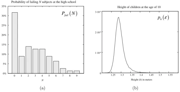
Figure 2.1: Examples of probability distributions for (a) a discrete variable (pmf) and (b) a continuous variable (pdf).

For a continuous variable x, the distribution is described by its probability density

function (pdf), denoted by px(ǫ) (note the uncapitalized p) which does not indicate

probabilities, but probability densities for each possible value ofx=ǫ. Here,

probabil-ities can be always obtained for the event that the variablex falls within a given range

[a, b] by means of:

P(a < x < b) =

Z b

a

px(ǫ)dǫ (2.2.1)

The concepts of pmf and pdf are illustrated with two realistic examples in the

Figure 2.1.

Another concept, related to the pdf through Lebesgue integration, is thecumulative

distribution function (cdf), which also fully describes a probability distribution by

measuring the probability of the variablexbeing below any given value. In the case of

(31)

Fx(ǫ) =P(x < ǫ) (2.2.2)

Obviously, the limit of a cdf must be zero and one for x tending towards minus

and plus infinity, respectively. A cdf may contain discontinuities, but continuity from

the right hand must be assessed for each of them [Apo07]. For the common case of a

continuous cdf, the probability of any given open set ]a, b[ will be always identical to

that of the closed set [a, b], since the Lebesgue measure of the end points a and b is

zero.

A distribution is said to bemultivariate when it describes the statistical occurrence

of more than one variables, which may be continuous, discrete or an arbitrary mixture

of them. The pdf (or cdf) of multiple variables is called ajoint distribution, in contrast

to a marginal distribution where only one of the variables is considered.

Another important concept is the mathematical expectation of any arbitrary

func-tion f(x) of a RV x, which determines the output from the function f(_·) that will be

closest, in average, to the output generated from random samples of x. It is denoted

with the E[_·] operator, defined as

Ex[f(ǫ)] =

Z ∞

−∞

f(ǫ)px(ǫ)dǫ (2.2.3)

Using this expectation we can define then’th (non-central) moment of a distribution

as:

µ′n=Ex[ǫn] (2.2.4)

The first of these moments (n = 1) is the mean of the distribution. Denoting

the mean of the RV x as ¯x we can now determine the n’th central moment of its

(32)

µn=Ex[(ǫ−x¯)n] (2.2.5)

In this case, the most widely employed moment is the second order one, named

variance, which measures the dispersion of the distribution. In the case of multivariate

distributions the moments become matrices, and the second central moment is called

the covariance matrix.

Regarding the probability distributions of two or more RVs, there exist a number

of fundamental definitions that will be used extensively throughout this thesis. They

are enumerated briefly below.

Conditional distribution: The conditional pdf of a RV ygiven another variable

x is written down as p(y|x), and can be shown to be:

p(y|x)=. p(x, y)

p(x) (2.2.6)

with p(x, y) being the joint pdf of both variables.

Independence: A pair of variables x and y are said to be independent if the information provide bdy one of them contributes nothing to the knowledge about the

other. Put mathematically, independent RVs fulfill:

p(y_|x) = p(y) (2.2.7)

p(x|y) = p(x) (2.2.8)

p(x, y) = p(x)p(y) (A consequence of Eqs. (2.2.6)–(2.2.7))

Conditional independence: A pair of variables x and y are conditionally inde-pendent given another third variable z if, given knowledge of z, further knowledge of

x ory gives no information abouty orx, respectively. This property will be discussed

(33)

Law of total probability: The pdf of a set of one or more RVs y can be always obtained by “averaging out” its conditional distribution p(y_|x) for any other arbitrary

set of RVs x, that is:

p(y) = Ex[y|x] =

Z _∞

−∞

p(y_|x)p(x)dx (2.2.9)

In the case of discrete variables, this law can be expressed as a sum:

P(y) =Ex[y|x] =

X

∀x

P(y|x)P(x) (2.2.10)

2.3 Parametric probability distributions

Probability distributions of random variables can be broadly divided into two

distinc-tive groups: parametric and non-parametric.

In the first case, the pmf or pdf governing the random variable can be described

through a mathematical equation that gives the exact value of the distribution for

the whole domain of the variable. In contrast, non-parametric distributions cannot be

modeled by formulas that yield directly and exactly their value, and other methods

must be employed instead as will be discussed below (_§2.4).

There exist dozens of well-known parametric distributions [Abr65,Eva01], although

in this work only a few will be employed, which are introduced below.

2.3.1 Uniform distribution

This is the simplest distribution, where all the potential values of a random variable z

(34)

16 Parametric probability distributions

z _{∼ U}(a, b) pz(x) =U(x;a, b) =

( ₁

b−a , forx∈[a, b]

0 , otherwise (2.3.1)

2.3.2 Normal or Gaussian distribution

Certainly the most widely employed density due to its remarkable properties, such as

the convenience of many operations such as summing, conditioning or factoring normal

variables also giving normal variables.

In this text, the fact that an N-dimensional random variable z with mean ¯z and covariance matrix Σz is governed by a Gaussian distribution will be denoted as:

z∼ N(¯z,Σz) (2.3.2)

with its pdf defined parametrically as:

pz(x) = N(x; ¯z,Σz) =

1 (2π)N/2p_|_Σ

z|

exp

−1

2(x−¯z)

⊤_Σ

z−1(x−¯z)

2.3.3 Chi-square distribution

Given a sequence ofkuni-dimensional normally-distributed variableszi with mean zero

and unit variance, the statistic

q=

k

X

i=1

z_i2 (2.3.3)

is also a random variable that follows a chi-square distribution with k degrees of

free-dom, that is,q _∼χ2

k. The density of this distribution, defined for non-negative numbers

only, is given by:

pq(x) =

xk/2−1_e−x/2

(35)

where Γ(k) is the gamma function, with no closed-form solution.

The importance of this density comes from it being the foundation of an important

method to compare two statistical distributions, named thechi-square test. This test is

widely employed in probabilistic robotics to deal with problems such as stochastic data

association (see [Nei01] and §14.6). In a chi-square test we are not directly interested

in the chi-square pdf, but rather on itsinverse cumulative distribution function, which

will be denoted asχ2

k,c. The test gives us the maximum value of the statistic q such as

it can be asserted that the two distributions being compared coincide with a certainty

of c(a probability between 0 and 1).

2.4 Non-parametric probability distributions

In spite of the wide applicability of the normal distribution, many continuous variables

in the real-world cannot be properly modeled as Gaussians or any other parametric

distribution. In those cases, non-parametric methods must be applied to model the

corresponding probability densities.

Kernel-based methods approximate the actual density distribution of a random

variable from a sequence ofindependent samples. A kernel function, usually a Gaussian

[Par62], is inserted at each sampled value, and the pdf estimation consists of the

average of all these kernels. Since in mobile robotics there are few situations ( [Lil07]

is an example) where we can draw a large number of independent samples from the

variables of interest, these methods have a modest presence in the field.

The most straightforward non-parametric estimators arehistograms (for 1-dimension)

or probability grids (for higher dimensions). Although such approximations did find

(36)

18 Mahalanobis distance

keeping the probability for each bin in the histogram (or cell in the grids) is

im-practical and wastes most of the computational and storage resources in, probably,

non-interesting parts of that space.

An alternative approach is importance sampling [Dou01], where the actual pdf is

approximated by a set of weighted samples (orparticles) which are usually concentrated

on the relevant areas of the state space. The validity of importance sampling is based

on the interesting property that any statistic Ex[f(x)] of a random variable x can be

estimated from a set of M samples x[i] _{with associated weights} _ω[i]_{, since it can be}

proven that

lim

M−→∞

M

X

i=1

ω[i]_f₍_x[i]_{) =} _E

x[f(x)] (2.4.1)

for the correct values of weights. In practice, the degree of accuracy attainable by

importance sampling is an important issue, since the number of samples must be kept

bounded due to computational limitations. Montecarlo simulation with importance

sampling is the base of particle filters, which will be discussed in _§2.7.2.

2.5 Mahalanobis distance

The Mahalanobis distance DM is a convenient measurement of distances from a fixed

pointyto another point xwhose location follows a normal distribution_N(¯x,Σx). For

two independent variables, this distance is given by:

DM (x,y) =

q

(y−x¯)⊤Σx−1(y−x¯) (2.5.1)

The intuitive idea behind the Mahalanobis distance is to account for distances

(37)

-4 -2 0 2 4 6 8 10

-2 -1 0 1 2 3 4 5 6 7 8 9

3 2 1

,

4 1 1

ª º ª º =« » =« » ¬ ¼ ¬ ¼ ȝ Ȉ 1 M D = 2 M D = 3 M D = ȝ

Figure 2.2: An example of the Mahalanobis distance for a 2-d Gaussian _N(µ,Σ). The ellipses represent the 68%, 95% and 99.7% confidence intervals for the random variable de-scribed by this Gaussian to be within the enclosed areas, forDM being 1, 2 or 3, respectively.

of constant Mahalanobis distance from the mean point of a 2-d Gaussian. These ellipses

will be often used to represent confidence intervals throughout this text.

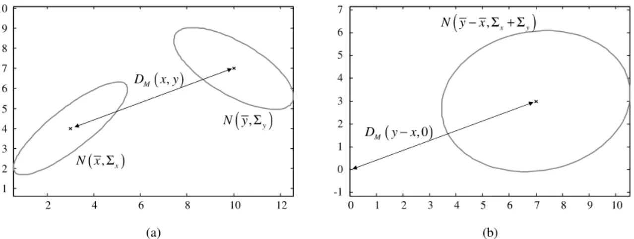
Another interesting application of the Mahalanobis distance is when both points x

and y are Gaussian random variables. In that case, the Mahalanobis distance can be

computed as:

DM(x,y) =

q

(¯y₋x¯)⊤(Σx+Σy−2Σxy)−1(¯y−x¯) (2.5.2)

with Σxy being the cross-covariance matrix of the two variables. This expression can

be easily derived by noticing that computing this distance between two Gaussians can

(38)

20 Kullback-Leibler divergence

2 4 6 8 10 12

1 2 3 4 5 6 7 8 9 10

0 1 2 3 4 5 6 7 8 9 10

-1 0 1 2 3 4 5 6 7

( , _x)

N x Σ

(

, y

)

N yΣ

( , )

M

D x y

( , 0)

M

D y−x

(

, _x _y

)

N y−x Σ + Σ

(a) (b)

Figure 2.3: (a) An example of the Mahalanobis distance between two Gaussiansxandy. (b) The same distance, reformulated as the distance to the origin from the variable representing the difference of both Gaussians.

2.6 Kullback-Leibler divergence

The Kullback-Leibler divergence (KLD) is a measure of the similarity between two

probability density functions p(x) andq(x), defined as [Kul51]:

DKL(p, q) =

Z _∞

−∞

p(x) logp(x)

q(x)dx (2.6.1)

Only two exactly equal densities give a KLD value of zero. Otherwise, the KLD is

always a positive quantity. In spite of the similarities with the mathematical definition

of a distance, the KLD is not a valid distance metric since, in general, DKL(p, q) 6=

DKL(q, p), hence the usage of the term divergence.

One application of KLD found in mobile robotics is to measure the similarity of

two independent N-dimensional Gaussian distributions p and q, that is, DKL(p, q),

(39)

p(x) = N(x;µp,Σp) (2.6.2)

q(x) = _N(x;µq,Σq)

which has the closed-form solution:

DKL(p, q) =

1 2

log |Σq|

|Σp|−

N + tr Σ−_q1Σp

+ (µq−µp)⊤Σq−1(µq−µp)

(2.6.3)

Another interesting situation where KLD finds applications is in comparing two

sums of Gaussians (SOG). Unfortunately, there is no closed-form expression in this

case, but an upper bound exists as proven by Runnalls in [Run07]. This result will be

useful in this thesis, as shown in §14.6.2.

2.7 Bayes filtering

The Bayes rule is the grounding of an important family of probabilistic estimation

techniques named Bayes filters which underlies many of the approaches presented in

this thesis. Given a probabilistic belief about the state x of a system, Bayes filtering

estimates the new belief after acquiring observations z that are directly or indirectly

related to the system. Put mathematically, the rule is stated as:

p(x_|z) =p(x)p(z|x)

p(z) (2.7.1)

The belief after incorporating the observation, that is, p(x|z), is referred to as the

posterior density, while the term p(x) is named the prior density and p(z|x), which

models how observations are related to the system state, is called the observation

likelihood. The denominator p(z), called the partition function in some contexts,

(40)

22 Bayes filtering

proper density function. As will be seen when discussing robot localization and SLAM

(in chapters 3 and 7, respectively), this Bayes rule can be applied recursively to the

sequence of variables in a dynamic system that evolves with time.

It is worthy to highlight a convention that will be used throughout this thesis: the

distribution that represents the knowledgebefore incorporating the new information in

the Bayes equation, that is, p(x) in Eq. (2.7.1), will be always called Bayes prior, or

just prior if there is no ambiguity. This remark is necessary since, strictly speaking,

“priors” are distributions not conditioned to any other variable, whereas it will be quite

common to find Bayes priors asp(x|B), withB being previous knowledge, e.g. already

incorporated in previous steps of a sequential Bayes filter.

Note that the Bayes rule states the relation between generic probability densities.

Each of the existing Bayesian filters specializes in approaching the problem for a

differ-ent represdiffer-entation of the densities, and/or for the cases of linear and non-linear models,

as briefly introduced in §§2.7.1–2.7.2. A deeper discussion about Bayesian filters can

be found elsewhere [Dou01, Ris04].

2.7.1 Gaussian filters

This family of Bayesian filters relies on multivariate Gaussian distributions to model

the uncertainty in all the variables of both the system state and the observations.

Systems with both linear transition and linear observation equations can be optimally

estimated by means of the Kalman filter (KF) [Kal60], which means that the posterior

converges towards the actual distribution as observations are processed.

The limitation of linear equations can be avoided by linearization, which leads to

the Extended Kalman Filter (EKF) [Jul97], or by systematic sampling, which gives the

(41)

(IKF) (which was proven to be equivalent to the Gauss-Newton method [Bel93]), and

the Information Filter (IF) [Wal07], which maintains and updates normal distributions

in their canonical form [Wu05].

2.7.2 Particle filters

The application of Monte-Carlo simulation to sets of particles with the aim of

approx-imating Bayes filtering leads to a group of techniques generically named particle filters

(PF) or Sequential Monte Carlo (SMC) estimation. The main advantages of PFs in

comparison to Kalman Filters are the avoidance of linearization errors and the

possi-bility of representing other pdfs apart from Gaussians. On the other hand, PFs require

a number of samples that grows exponentially with the dimensionality of the problem.

In its simplest form, a PF propagates the samples that approximate the prior in the

state space using the transition model of the system, and then updates their weights

using the observation likelihood. A detailed survey of particle filtering techniques can

be found in Chapter 4, where we also propose a novel particle filter algorithm.

As an additional remark, in most practical situations (where linear models are

not applicable) Monte-Carlo simulation with a large enough number of samples is

usually considered the standard for approximating the ground-truth distribution of

(42)

24 Resampling strategies

2.8 Resampling strategies

A common problem of all particle filters is the degeneracy of weights, which consists

of the unbounded increase of the variance of the weights ω[i] _{with time}2_{. In order to}

prevent this growth of variance, which entails a loss of particle diversity, one of a set

of resampling methods must be employed.

The aim of resampling is to replace an old set of N particles by a new one with the

same population size but where particles have been duplicated or removed according

to their weights. More specifically, the expected duplication count of the i’th particle,

denoted by Ni, must tend to N ω[i]. After resampling, all the weights become equal

to preserve the importance sampling of the target pdf. Deciding whether to perform

resampling or not is most commonly done by monitoring theeffective sample size (ESS)

[Liu96], obtained from theN normalized weights ω[i] _as:

ESS =

N

X

i=1

(ω[i])2 !−1

∈[1, N] (2.8.1)

The ESS provides a measure of the variance of the particles’ weights, e.g. the

ESS tends to 1 when one single particle carries the largest weight and the rest have

negligible weights.

2.8.1 Overview

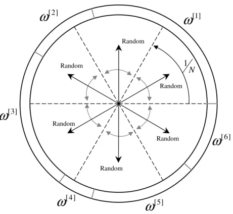
This section describes four different strategies for resampling a set of particles whose

normalized weights are given byω[i]_{, for}_i_{= 1}_{, ..., N}_{. The methods are explained using}

a visual analogy with a “wheel” whose perimeter is assigned to the different particles in

such a way that the length of the perimeter associated to each particle is proportional to

2

(43)

its weight (see Figures 2.4–2.7). Therefore, picking a random direction in this “wheel”

implies choosing a particle with a probability proportional to its weight. For a more

formal description of the methods, please refer to the excellent paper by Douc, Capp´e

and Moulines [Dou05].

[1]

ω

[2]

ω

[3]

ω

[4]

ω

[5]

ω

[6]

ω

Random

Figure 2.4: The multinomial resampling algorithm.

• Multinomial resampling: It is the most straightforward resampling method, whereN independent random numbers are generated to pick a particle from the

old set. In the “wheel” analogy, illustrated in Figure 2.4, this method consists

of picking N independent random directions from the center of the wheel and

taking the pointed particle. The name of this method comes from the fact that

the probability mass function for the duplication counts Ni is a multinomial

(44)

[1]

ω

[2]

ω

[3]

ω

[4]

ω

_ω

[5]

[6]

ω

Random

[1]

ω

[2]

ω

[3]

ω

[4]

ω

_[5]

ω

[6]

ω

Figure 2.5: The residual resampling algorithm. The shaded areas represent the integer parts of ω[i]/(1/N). The residual parts of the weights, subtracting these areas, are taken as the modified weights ˜ω[i].

• Residual resampling: This method comprises two stages, as can be seen in Figure 2.5. Firstly, particles are resampled deterministically by picking Ni =

⌊N ω[i]_⌋ _{copies of the} _i_{’th particle. Then, multinomial sampling is performed}

with the residual weights:

˜

(45)

[1]

ω

[2]

ω

[3]

ω

[4]

ω

[5]

ω

[6]

ω

Random

Random Random

Random 1

N

Figure 2.6: The stratified resampling algorithm. The entire circumference is divided into

N equal parts, represented as the N circular sectors of 1/N perimeter lengths each.

• Stratified resampling: In this method, the “wheel” representing the old set of particles is divided into N equally-sized segments, as represented in Figure 2.6.

Then, N numbers are independently generated from a uniform distribution like

in multinomial sampling, but instead of mapping each draw to the entire

cir-cumference, they are mapped within its corresponding partition out of the N

(46)

[1]

ω

[2]

ω

[3]

ω

[4]

ω

[5]

ω

[6]

ω

1 N

1 N 1

N

Random

Figure 2.7: The systematic resampling algorithm.

• Systematic resampling: Also calleduniversal sampling, this popular technique draws only one random number, i.e. one direction in the “wheel”, with the

othersN−1 directions being fixed at 1/N increments from that randomly picked

direction.

2.8.2 Comparison of the four methods

In the context of Rao-Blackwellized particle filters (RBPF) [Dou00a], where each

par-ticle carries a hypothesis of the complete history of the system state evolution,

re-sampling becomes a crucial operation that reduces the diversity of the PF estimate

(47)

loss, the four different resampling methods discussed above have been evaluated in a

benchmark [Bla09a] that measures the diversity of different states remaining after t

time steps, assuming all the states were initially different.

The results, displayed in Figure 2.8, agree with the theoretical conclusions in

[Dou05], stating that multinomial resampling is the worst of the three methods in

terms of variance of the sample weights. Therefore, due to its simple implementation

and good results, the systematic method is employed in the rest of this work when

eval-uating “classical” particle filters, in constrast to our new proposed algorithms where

resampling is addressed differently, as explained in the corresponding chapters.

101

102

100 ₁₀1

1

Time steps (t)

Number of hypotheses surviving since t=1

Multinomial Residual Stratified Systematic

(48)

30 Random sample generation

2.9 Random sample generation

A recurrent topic throughout probabilistic mobile robotics is drawing samples from

some probability distribution. Typical applications include Monte Carlo simulations

for modeling a stochastic process and some steps within particle filtering.

The most basic random generation mechanism is that for uniform distributions over

integer numbers, since any other discrete or continuous distribution can be derived

from it. Due to its importance, most modern programming languages include such

a uniform random generator. In the case of C or C++, the POSIX.1-2001 standard

proposes a simple pseudorandom generator – the implementation of the function rand

in the default C libraries. However, this method has its drawbacks in both efficiency

and randomness [Wil92].

In this thesis it has been employed an alternative method, namely the MT19937

variation of the Mersenne twister algorithm [Mat98]. Note that although this method

generates integer numbers, generating uniformly-distributed real numbers from them

is trivial. An application of uniform sampling in the context of resampling has been

already discussed in _§2.8.

Another distribution useful in probabilistic robotics is the 1-dimensional normalized

Gaussian, that is, with mean zero and unit variance, which can be obtained from

uniformly-distributed numbers following the algorithm gasdev described in [Wil92].

Drawing samples from multivariate Gaussians is the most important sampling

method in our context, since it is involved in most particle filters for robot

local-ization and mapping (e.g. for drawing samples from the motion models). Let ¯x and

Σx denote the mean and covariance, respectively, of theN-dimensional Gaussian from

(49)

x_{∼ N} (x¯,Σx) (2.9.1)

If we obtain the N eigenvaluesei and eigenvectorsvi ofΣx, thek’th element of the

sample xis given by

x(k) = ¯x(k) +

N

X

i=1

√

eivi(k)rk (2.9.2)

where each rk is a random sample from a 1-dimensional, normalized Gaussian. This

method can be seen as a change of bases from the N-hypersphere where the N

in-dependent and identically distributed (i.i.d.) random samples rk are generated, into

the orthogonal base defined by the eigenvectors of the covariance matrix Σx, each

dimension scaled by the corresponding eigenvalue.

2.10 Graphical models

Graphical models are a powerful tool where concepts from both graph and

probabil-ity theories are applied in order to make efficient statistical inference or sampling in

problems involving several random variables [Bis06, Jen96]. In this paradigm, a graph

represents a set of random variables (the nodes) and their statistical dependencies (the

edges). Graphical models have recently inspired interesting approaches in the mobile

robot SLAM community [Cum08,Pas02]. Furthermore, some well-known methods such

as the Kalman filter or Hidden-Markov models can be shown to be specific instances

of inference on graphical models [Bis06].

(50)

32 Graphical models

as a Bayesian network (BN) or a Markov random field, respectively. In this work we

are only interested in BNs, where the direction of edges can be interpreted as a causal

relation between the variables that gives raise to a statistical dependence.

To illustrate the usage of a BN to, for example, factor a joint distribution, consider

the example in Figure 2.9 with the five random variables _{a, b, c, d, e_}:

a b c

e d

Figure 2.9: An example of a Bayesian network with five random variables.

Given the dependencies in this graph, the joint distribution of the system can be

factored exploiting thelackof connections between some nodes. In the current example,

using the Law of Total Probability we arrive at:

p(a, b, c, d, e) = p(a)p(d)p(b|a)p(c|b)p(e|a, d). (2.10.1)

Another important information that can be determined from a BN is whether two

variables (or sets of variables 3₎ _a _and _c _are _{conditionally independent} _{given another}

set of variables b, what is sometimes denoted as [Daw79]:

a ⊥⊥c| b (2.10.2)

This condition can be asserted from the BN by inspecting whether the fixation of

the values of the variables inb leaves no connection that could carry information from

3

(51)

variables inato those inc, or whether the arrows (in the possible paths betweena and

c) meet head-to-head at some intermediary node that is not part of b. If at least one

of those two conditions holds, it is said that b d-separates a and c. For a more formal

definition of the rules to determine d-separation, please refer to [Bis06, Rus95b, Ver90].

A pair of variables a and d (refer to Figure 2.9) can be also (unconditionally)

independent, which can be denoted as a_⊥⊥ d _| ∅ or simply a _⊥⊥d. From the rules to

determine d-separation, it can be deduced that two variables are independent only if

all the paths between them end in a head-to-head arrow configuration (or, obviously,

when there is no connection at all between them).

Summarizing for the example in Figure 2.9, it can be observed that b d-separates

a and c, thus a _⊥⊥ c _| b, and therefore the distribution p(a, c_|b) can be factored as

p(a_|b)p(c_|b). Moreover, it can be observed thata and dare (unconditionally)

indepen-dent variables (since the arrows in the patha _↔d meet head-to-head), that is, a_⊥⊥d,

and hence p(a, d) =p(a)p(d).

The application of these simplifications is at the core of many modern approaches

(52)

(53)

Part I

Mobile Robot Localization

(54)

(55)

CHAPTER 3 OVERVIEW

This chapter briefly reviews the problem of mobile robot localization and some of the

existing solutions proposed in the literature.

In general, the reported methods can be divided into those based on metric maps

(e.g. sets of landmarks, occupancy grids) and those relying on topological maps (e.g.

a graph of distinctive “places”). Although the latter approach has led to some

success-fully localization frameworks [Cum08, Kui90], the largest part of the literature focuses

on pure metric methods due to their better suitability to indoor, possibly cluttered

(and dynamic) spaces where a mobile robot needs an accurate pose estimation in order

to perform some basic tasks such as motion planning.

Metric localization most commonly addresses the problem of pose tracking, where

an estimate of the robot pose is sequentially updated as new data are gathered by

the sensors (e.g. wheels odometry, camera images or laser scans). This situation can

be characterized by the existence of a unique robot pose hypothesis relatively well

(56)

38

x_t-1 x_t x_t+1

u_t u_t+1

u_t-1

… …

z_t-1 z_t z_t+1

m

Robot poses

Figure 3.1: The dynamic Bayesian network for mobile robot localization, where robot poses

xtare hidden variables (represented as shaded nodes) to be estimated from actionsut, sensor

observationszt and a model of the environmentm.

localized in space. An extension of this paradigm is global localization, the problem

of a robot “awakening” in an unknown position of the environment. In this case, a

multitude of localization hypotheses must be managed simultaneously.

Bayesian filtering allows the coherent treatment of both, global localization and

pose tracking in a single probabilistic framework. Although parametric filters such as

multihypotheses Kalman filters have been used for this aim [Arr02a], the most common

approach is particle filtering [Thr05].

Mathematically, probabilistic robot localization consists of estimating the

distribu-tion of a hidden dynamic variable xt, standing for the robot pose at time step t, given

sensor observations zt, a map of the environment m and robot actions ut (normally,

odometry increments).

From the dynamic Bayesian network (DBN) of the problem, displayed in Figure 3.1,

it is clear that the sequence of robot poses constitute a Markov process, that is, given

a posext, the pose at the next instant xt+1 is conditionally independent of all previous

(57)

3. Overview 39

xt+1 ⊥⊥x1, x2, ..., xt−1 | xt. (3.0.1)

Therefore, the problem can be addressed sequentially by estimating one robot pose

at once based on the previously estimated pose, using the well-known expression:

p(xt|z1:t, u1:t, m)∝p(zt|xt, m)

Z

p(xt|xt−1, ut)p(xt−1|z1:t−1, u1:t−1, m)dxt−1 (3.0.2)

The derivation of this equation is given next along a detailed description of the

probabilistic rules applied in each step. Note that superscripts have been used for

shortening the expressions with sequences of variables, e.g. xt₌. _x

1:t.

p(xt|zt, ut, m)

| {z }

Posterior fort

∝

Bayes onzt p(zt|xt, zt−1, ut, m)p(xt|zt−1, ut, m) =

zt⊥⊥zt−1, ut|xt, m p(zt|xt, m)

| {z }

Observation likelihood

p(xt|zt−1, ut, m) =

Law of total

probability onxt−1 p(zt|xt, m)

Z _∞

−∞

p(xt|xt−1, zt−1, ut, m)p(xt−1|zt−1, ut, m)dxt−1 =

xt⊥⊥zt−1, ut−1, m|xt−1, ut p(zt|xt, m)

Z ∞

−∞

p(xt|xt−1, ut)

| {z }

Motion model

p(xt−1|zt−1, ut, m)dxt−1 =

xt−1⊥⊥ut|∅ p(zt|xt, m)

Z _∞

−∞

p(xt|xt−1, ut)p(xt−1|zt−1, ut−1, m)

| {z }

Posterior fort−1

dxt−1

In the next chapter it is explored a novel algorithm for effective Bayesian filtering

(58)

40

for a new observation model useful for localization with accurate laser range scanners

in dynamic environments. Finally, we also address in Chapter 6 the issue of improving

(59)

CHAPTER 4 OPTIMAL PARTICLE

FILTERING FOR

NON-PARAMETRIC

OBSERVATION MODELS

4.1 Introduction

Sequential estimation of dynamic, partially observable systems is a problem with

nu-merous applications in a wide range of engineering and scientific disciplines. The

state-space form of this problem consists of iteratively tracking the state of a system at

discrete time steps given the system transition and observation models and a sequence

of observations. In a probabilistic framework, sequential Bayesian filtering represents

(60)

42 Introduction

an effective solution [Liu98, Dou01, Ris04].

In the scope of mobile robotics there are two prominent applications of Bayesian

sequential estimation that have received a huge attention by the research community

in the last decade, namely localization and simultaneous localization and map

build-ing (SLAM) [Thr01b, Thr05, Est05, Gut99, Fox99b, Dis01, Hah03, Thr02, Gri07b]. As

discussed in Chapter 3, the former consists of estimating the pose of a mobile robot

within a previously known environment, whereas in SLAM a map of the environment

is estimated from scratch while performing self-localization.

In both cases the choice for the representation of the environment determines which

Bayesian estimation method can be applied. For example, landmark maps can be

modeled by multivariate Gaussian distributions with Gaussian observation models that

can be obtained by solving the data association problem [Dis01, Dav07]. Therefore,

SLAM with landmark maps can be solved through Gaussian filters such as the EKF

[Jul97] or the UKF [Wan00]. However, for other types of map representations, like

occupancy grid-maps [Mor85,Thr03], these filters are not applicable, forcing a

sample-based representation of probability densities and sequential estimation carried-out via

Monte-Carlo simulations (the filtering algorithms becomes a particle filter [Dou01]).

In this chapter we focus on occupancy grids as map model, although the described

method, published in [Bla08h], can be also applied to other maps compatible with a

sample-based representation of probability distributions (e.g. gas concentration maps

[Lou07], topological maps [Ran06]). Among the advantages of mapping with occupancy

grids we find the precise dense information they provide and the direct relation of

the map with the sensory data, which avoids the problem of data association that

is present in landmark maps [Nei01]. Their main drawback is that the observation

likelihood model for grid maps can be evaluated only pointwise in a non-parametric

Contributions to Localization, Mapping and Navigation in Mobile Robotics