The Use of Machine Learning Algorithms for
the Study of Business Profitability: A New
Approach Based on Preferences
Javier de Andrés. University of Oviedo. Spain. jdandres@uniovi.es
Pedro Lorca. University of Oviedo. Spain. plorca@uniovi.es
Antonio Bahamonde. University of Oviedo. Spain. antonio@aic.uniovi.es
Juan José del Coz. University of Oviedo. Spain. juanjo@aic.uniovi.es
Abstract. In recent years, researchers in the field of Artificial Intelligence have developed a learning technique, namely, preference learning, that is suitable to be used for economic analysis. The present research empirically tests one of these models, which consists of a combination of LACE and RFE algorithms. The problem of forecasting the profitability of Spanish companies upon the basis of a set of financial ratios is used as a benchmark. The model provides forecasted rankings, which are a kind of information that is more useful for the economic analysts than the forecasted class memberships that traditional machine learning techniques provide.
Keywords: profitability, machine learning algorithms, preference learning, financial ratios.
1. INTRODUCTION
Classification techniques and regression analysis are the two most popular approaches between financial analysts and researchers for the analysis and forecasting of certain economic phenomena, such as financial health or business
profitability. The aim of the use of classification systems is to predict which category an individual/company/country will belong to in the future from a closed list of several possible ones, upon the basis of the levels of the predictors. The classification systems that financial analysts and researchers use more frequently are statistical techniques, such as, for example, discriminant analysis or logistic regression (Altman et al., 1977; Martin, 1977, and many others), classifier neural networks (Tsai, 2000; Mak and Munakata, 2002, among others), and rule induction systems (i.e., Markham et al., 2000; Mak and Munakata, 2002).
When the economic phenomenon that we are trying to forecast can be represented through a continuous variable, the use of regression models seems preferable at first. Many regression models have been developed, from the commonly used ordinary least squares functions to the different systems based in predictive neural networks and fuzzy sets (see, for example, Kosko, 1992). But very often regression leads to poor results, as the functional form of the relationship between many economic and financial variables is not easy to determine. As we will explain in section 2, this is the case in respect of profitability analysis.
Whenever regression fails, a possible solution is to discretize the variable which we are trying to forecast and construct a classification system. So, we pursue a second-order objective which is to predict only the position of the firm, described using a range of a few possible states, but not the exact value for the forecasted variable. The rationale for this approach is reinforced by the fact that classification can be understood as a special case of regression where the dependent variable is categorical.
However, it can be argued that the discretization procedures based on the above argument imply loss of information, and so diminish the power of the constructed model for economic and financial analysis. This drawback was pointed out by the early researchers into bankruptcy prediction (see, for example, Eisenbeis, 1977).
classification systems, but there is no need to determine the exact functional form of the relationship among the variables under study.
The use of an approach based on preferences has provided good results in other fields (see, e.g., Herbrich et al., 1999, for an application to the modelling of consumers’ behavior). In the present paper, we test the usefulness of this approach for financial analysis. We use a combination of two algorithms: LACE (Learning to Assess from Comparison Examples, Díez et al., 2002) and RFE (Recursive Feature Elimination, Guyon et al., 2002). The task we deal with is profitability analysis. This is an issue that traditionally has been studied using classification models, as regression analysis has failed to produce good results. As the outcome of the approach based on preferences is a forecasted ranking rather than a forecasted value or a forecasted membership, it is not possible to compare its results neither with those of regression analysis nor with the accuracy of classification models such as discriminant analysis, logit or machine learning classifiers.
The remainder of the paper is structured as follows: in section 2, prior research into profitability analysis is briefly reviewed, and section 3 explains the comparisons approach and the two algorithms used in the present research. Section 4 discusses the methodology of the study. The main results are expounded in section 5, and section 6 is devoted to the summary and conclusions of our research work.
2. PRIOR RESEARCH ON PROFITABILITY
FORECASTING
The prediction of the future profitability of non-financial firms is an issue that has received a considerable amount of interest on the part of researchers in the financial field. Early works on this issue (e.g., Gort, 1963; Harris, 1976), tried to explain profitability through regression analysis. This led to poor results, mainly due to the following reasons:
a) Economic theory does not provide any guide to the selection of the function which best represents the relation between the predictors and profitability.
the listed companies of a certain market/country, the researchers had to consider firms of different branches of activity in order to attain a sample with a sufficient number of firms to guarantee the statistical validity of the analysis.
So, the principal conclusion of the papers that used regression was that it is not possible through a function to obtain reliable predictions of the exact level of profitability of a certain firm. In consequence, researchers then pursued a second-order objective, that is, the determination of the features that most distinguish profitable from unprofitable firms. This approach had previously been used for the analysis of certain economic variables in certain environments, such as, for example, the earnings-price ratio of listed firms (Walter, 1959) and the performance of commercial banks (Haslem and Longbrake, 1971).
The above procedure implies loss of information as well as a certain degree of subjectivity in the methodology. This is because the forecasted variable has to be discretized to form classes, and the criteria for the discretization must be established by the researcher, as there are no generally accepted guidelines for class identification. Thus, Gillingham (1980), who studied profitability through discriminant analysis, considered profitable firms those having positive earnings before taxes; if this were not so, firms were unprofitable. Chaganti and Chaganti (1983), who used discriminant analysis, defined three classes: very profitable firms, which were companies with financial profitability above 13%; moderately profitable firms, for which financial profitability was between 0% and 13%; and unprofitable firms, which were firms with negative net profit.
This procedure also has the additional drawback of inducing low separability between the classes. As the breakpoints are arbitrarily established, no significant differences should exist between the companies around those points. However, this methodology is still used in papers on firm performance (e.g., Shipchandler and Moore, 2000).
An example of this is the study by Woo (1983), who identified high profitability firms as those with Return On Investments (ROI) above 40%, while low profitability firms had ROI under 10%. This author discarded the rest of the companies, and so attained through discriminant analysis an improved accuracy over that of previous papers.
More recently, other authors followed an alternative version of this approach which consisted of discretizing profitability by using a descriptive statistic rather than establishing fixed intervals. For example, Weir (1996), who estimated a logit function, defined high profitability as profitability that is above the sectoral mean. In the same manner, De Andrés (2001) and De Andrés et al. (2002, 2003, 2004), who tested the accuracy of several machine learning rule inductors, identified the classes through a measure based on the percentiles of the statistical distribution of financial profitability.
In general, all these papers provide a valid but incomplete approach to the understanding of the profitability phenomenon. The classification systems that are obtained predict with an acceptable accuracy if a company will belong in the future to a certain profitability group, but do not allow researchers and financial analysts to rank the companies within a certain class. This is a serious drawback because in the “real life” investors have a limited amount of capital to invest. So, they need to rank companies and select the best, and not only identify profitable investments.
Until recent years this could be done only by using a regression approach which, as seen above, did not lead to good results. But the development of preference learners puts very powerful tools at the researchers’ disposal, as these models allow analysts to rank the companies without the extra burden of predicting the future value of their profitability of the firms. The following section briefly reviews these algorithms.
3. ALGORITHMS FOR LEARNING PREFERENCES
relations between characteristics described by the components of real number vectors. In our problem, v and u are vectors describing features of two companies that are being compared, with the result that v is better (more profitable) than u.
This learning task can be accomplished by taking two approaches. We may look for classifiers to decide whether a pair (v, u) belongs or not to the relation, as in Utgoff and Saxena (1987) and Branting and Broos (1997). In general, the relation so induced is not transitive. However, Cohen et al. (1999), describe an algorithm that heuristically finds a good approximation to the ordering that best agrees with the learned binary relation.
The second approach tries to find a ranking function f able to assign a real number to each vector in such a way that preferable characteristics obtain higher values. This path is followed by several authors (e.g., Tesauro, 1998; Branting, 1999; Herbrich et al., 1999; Joachims, 2002); using different tools they propose algorithms to find a suitable linear function capable of ranking characteristics. This is also the approach followed by LACE (Díez et al., 2002).
3.1. LACE: Learning linear preference assessments
Let us assume that,
is a sample of an ordering relation in called preference relation. Our aim is to find an ordering preserving (monotone) function that will be called the assessment or ranking function. In other words, we look for a function f which maximizes the probability of having f ( v ) > f ( u ) whenever v is better than u.
The assessment of a vector x can be defined as its distance from an assessment hyperplane (Herbrich et al., 1999; Fiechter and Rogers, 2000; Joachims, 2002; Díez et al., 2002). From a geometrical point of view, the function represents the distance from the hyperplane (of vectors perpendicular to w) multiplied by the norm of w (see Figure 1).
Figure 1 We are looking for a vector w such that the hyperplane is farther from preferable vectors. In the picture v is better than u, in symbols, v > u
The core idea is that we can specify fw taking into account that
The search for w is an NP-hard problem; however, it is possible to approximate the solution. In LACE, the procedure followed to find a linear function with coefficients w = (w1, …, wd) is taken from OC1 (Murthy et al., 1994), only slightly modified for this purpose. In fact, what we are looking for is a vector w such that as many times as possible. We can start with w being the average of the normalized differences:
.
Now we try to improve the coefficients of w, one at a time. The key observation
is that for each normalized difference we have
that
(2)
(3)
when xj > 0, is equivalent to
or the opposite when xj < 0. When xj = 0, the value of the coefficient wj does not matter. So, for fixed values of all other coefficients, each equation (5) represents a constraint on the values of wj. Therefore, we sort all C values and consider as possible settings for wj the midpoints between each pair of consecutive C’s. We select the wj that satisfies the greater number of constraints. Following this procedure, we iterate this step in order to adjust all the coefficients until no further optimisation can be achieved.
3.2. Feature selection for learning preferences
As machine learning algorithms are applied to real-world tasks, one difficulty is selecting the best features to use for learning from a set of candidate attributes. Learners’ generalization performances can be improved when they are given only the information supplied by relevant features. Unfortunately, the opposite often occurs: an attribute that is irrelevant is not useful for induction and can degrade future accuracy.
Feature Subset Selection (FSS) is the process of identifying and removing as many of the irrelevant features as possible. In this paper, we introduce a technique that can determine how many features are significant for characterizing profitability forecasting. This technique uses the Recursive Feature Elimination algorithm (RFE) (Guyon et al., 2002), which produces an ordering of the features according to their usefulness.
RFE is an example of a backward feature elimination process. So, it starts with all possible features and removes one feature per iteration, the one with the smallest feature ranking criterion. When the ranking function is linear, RFE’s criterion is the value of (wi)2, where w
i is the coefficient of the i-th feature in the function induced by LACE. A theoretical justification for using this criterion can be found in Guyon et al. (2002). See also Rakotomamonjy (2003) for further experimental results.
This algorithm lets us obtain a ranked list L=(Fd, Fd-1,…,F1) with d different feature subsets, where each Fi is a subset with exactly i features. Due to the recursive
elimination, features in a subset Fi are optimal in some sense when considered together, although individually they could be less relevant than other features eliminated in a previous step. This is an interesting property of RFE since it takes into account possible relations between features, making feasible the possibility of discovering useful groups of interrelated features that would be labeled as irrelevant if considered one by one. However, it should be noted that, given the greedy nature of RFE, Fi will not necessarily contain the i most useful features of the original feature set in order to achieve a higher accuracy.
Once the ranked list of feature subsets is obtained by means of RFE, the next step is to select one of them. In general, we will be interested in a subset which lets LACE learner yield the best performance, in terms of accuracy; so we need to estimate the performance for every feature subset.
A more reliable alternative to training error and other accuracy estimators is the metric-based method called ADJ (ADJusted distance) (Schuurmans, 1997; Schuurmans and Shouthey, 2002), devised to choose the appropriate level of complexity required to fit the data. In our case, given the nested sequence of feature
subsets obtained by RFE, , ADJ will provide a procedure to
select one of the hyperplanes wFi induced by LACE from the corresponding Fi. The key idea is the definition of a metric on the space of hypotheses. Thus, the distance between two given hypotheses wFi and wFj, is calculated as the expected disagreement in their predictions:
where err(wFi(x), wFj (x)) is the measure of disagreement on a generic point x in the space of example descriptions. Given that these distances can only be approximated, ADJ establishes a method to compute
d’
(
wFi , W), an adjusted-distance-estimatebetween any hypothesis wFi and the true target classification function W. Therefore, the selected hypothesis is:
.
The estimation of distance d’ is computed by means of the expected disagreement in the predictions in a pair of sets: the training set T, and a set U of unlabeled examples, that is, a set of cases sampled from Px but for which the
(6)
expected correct output is not given. The ADJ estimation is given by:
where, for a given subset of examples S,
d
S(
wFk , wFi ) is the expected disagreement of hypotheses wFk and wFi in S. Our proposal here is to use the Laplace correction to the probability estimation, in symbols:.
Notice that, in this way, we avoid the impossibility of using (8) when there are zero disagreements in T for two hypotheses.
In general, it is not straightforward to obtain a set of unlabeled examples, so Bengio and Chapados (2003) proposed a sampling method for the available training set. However, for learning preferences, we can easily build the set of unlabeled examples from a set of preference judgments formed by pairs of real objects randomly selected from the original preference judgments pairs. We fix the size of U to be 10 times the size of T.
4. METHODOLOGY
Once a brief overview on the algorithm for learning preferences has been provided, the remainder of the paper is devoted to commenting on the empirical tests that were carried out to determine the suitability of these techniques for the forecasting of business profitability. This section describes the methodology of the tests, and section 5 contains the comments on the results.
4.1. The data base
The information used was taken from the financial statements of commercial and industrial firms located in Spain. In accordance with Spanish legislation, limited liability companies are required to deposit their annual accounts in the Registro Mercantil (Commercial Register). This information is gathered and provided by Bureau van Dijk and Informa for Spanish firms in the Sistema de Análisis de Balances Ibéricos (SABI) data base. The financial statements analysed here correspond to the years 1998, 1999, 2000 and 2001.
(8)
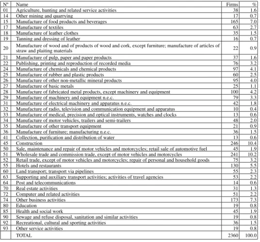
We considered only companies with more than 100 employees and fewer than 250. This is because, under Spanish legislation, companies under 100 employees do not have the obligation to submit their accounts to an auditor’s judgment, so their financial information is not reliable enough. The reason for the deletion of the companies with more than 250 employees is that big firms are usually multi-activity firms. This, in the absence of segment information, may cause distortions in the analysis. This holds especially in our case. As will be explained in subsection 4.4, the sectoral ascription is a key variable in some of the tests conducted.
Nº Name Firms %
01 Agriculture, hunting and related service activities 38 1.6
14 Other mining and quarrying 17 0.7
15 Manufacture of food products and beverages 165 7.0
17 Manufacture of textiles 63 2.7
18 Manufacture of leather clothes 35 1.5
19 Tanning and dressing of leather 16 0.7
20 Manufacture of wood and of products of wood and cork, except furniture; manufacture of articles of straw and plaiting materials 22 0.9
21 Manufacture of pulp, paper and paper products 37 1.6
22 Publishing, printing and reproduction of recorded media 76 3.2
24 Manufacture of chemicals and chemical products 97 4.1
25 Manufacture of rubber and plastic products 60 2.5
26 Manufacture of other non-metallic mineral products 95 4.0
27 Manufacture of basic metals 25 1.1
28 Manufacture of fabricated metal products, except machinery and equipment 100 4.2
29 Manufacture of machinery and equipment n.e.c. 79 3.3
31 Manufacture of electrical machinery and apparatus n.e.c. 42 1.8 32 Manufacture of radio, television and communication equipment and apparatus 10 0.4 33 Manufacture of medical, precision and optical instruments, watches and clocks 13 0.6 34 Manufacture of motor vehicles, trailers and semi-trailers 48 2.0
35 Manufacture of other transport equipment 21 0.9
36 Manufacture of furniture; manufacturing n.e.c. 36 1.5
41 Collection, purification and distribution of water 13 0.6
45 Construction 246 10.4
50 Sale, maintenance and repair of motor vehicles and motorcycles; retail sale of automotive fuel 45 1.9 51 Wholesale trade and commission trade, except of motor vehicles and motorcycles 241 10.2 52 Retail trade, except of motor vehicles and motorcycles; repair of personal and household goods 75 3.2
55 Hotels and restaurants 130 5.5
60 Land transport; transport via pipelines 55 2.3
63 Supporting and auxiliary transport activities; activities of travel agencies 53 2.2
64 Post and telecommunications 14 0.6
70 Real estate activities 31 1.3
72 Computer and related activities 51 2.2
74 Other business activities 173 7.3
80 Education 19 0.8
85 Health and social work 45 1.9
90 Sewage and refuse disposal, sanitation and similar activities 19 0.8
92 Recreational, cultural and sporting activities 36 1.5
93 Other service activities 19 0.8
TOTAL 2360 100.0
Table 1 Companies in the sample detailed by branch of activity
whenever any of the years in question (1998, 1999, 2000 and 2001) was the first year of business, or (c) when the information they provided was not enough to compute the selected ratios. After this pruning, the database was made up from the accounts of 2,360 Spanish companies. In table 1, the number of companies included in each NACE sector (Nomenclature générale des Activités économiques dans les Communautés Européennes, two digits) are shown.
4.2. Profitability
In order to measure the profitability of the firms, and taking into account informational limitations (only annual accounts were available), we chose the financial profitability ratio. This is defined as the quotient between the company’s net profit and equity capital. A considerable amount of literature (e.g., Kelly and Tippet, 1991; Brief and Lawson, 1992, among many others) suggests that, despite its limitations, this ratio provides a suitable measure of management efficiency.
For our study, we have considered the average profitability for the years 2000 and 2001. In our opinion, computing the variables in an averaged way is better than taking the data from the most recent year, as this procedure eliminates, at least partially, the undesirable distortions in the accounting figures caused by non-permanent changes in the environment of the firm.
1st Quartile 0.031
Median 0.074
3rd Quartile 0.136
Mean 0.095
Standard Deviation 0.151
Skewness -0.191
Kurtosis 29.555
Table 2 Descriptive information on the profitability of the analyzed companies
This preliminary finding gives us an additional reason for the poor results of the techniques such as regression analysis that predict the absolute value for the profitability of the firms. If almost all the observations are concentrated around the mean, predicting the mean for all the firms will produce low error rates, but this is of no use for economic analysis.
4.3. The predictors
As the aim of the research is to predict future profitability on the basis of the present financial and economic position of a firm, we started by choosing the financial aspects to be measured. We discarded as acceptable predictors those figures that could not be measured upon the basis of the information in the annual accounts drawn up according to the Spanish Generally Accepted Accounting Principles.
As was shown in section 2, the study of business profitability is not an easy task. After extensive consideration of prior literature, we selected 8 financial dimensions with potential power as predictors of profitability. These features are the following: (1) Debt quality, (2) Indebtedness, (3) Use of fixed capital, (4) Debt cost, (5) Short-term liquidity, (6) Share of labour costs, (7) Size, and (8) Average sales per employee.
In order to include the above features in our model, we selected, for each concept, the financial variable that best measured it. Again, we were faced with the limitations caused by the relatively small amount of information in Spanish accounts. In order to avoid multi-collinearity, each dimension is represented by one financial ratio. The chosen ratios were the most significant in prior studies on the profitability of medium-sized firms (e.g., Gillingham, 1980; De Andrés, 2001, De Andrés et al., 2002). The prediction set finally selected appears in Table 3. As can be seen, the different variables are labeled with the codes V1 to V8.
Dimension Variable Code
Debt quality V1
Indebtedness V2
Use of fixed capital V3
Debt cost V4
Short-term liquidity V5
Share of labour costs V6
Size Net Sales (EUR thousands) V7
Average sales per employee V8
Table 3 The set of financial variables
Apart from these variables, we have computed an additional set of predictors with the aim of avoiding the distortions caused by the so-called ‘sector effect’. In order to do this, we divided each one of the ratios by the median of the distribution for each branch of activity. This procedure has been successfully used in several studies of financial distress prediction (Izan, 1984; Platt and Platt, 1990). These eight ‘relative’ indicators have been labeled RV1 to RV8. The way this additional set is considered for the analysis will be explained in the next subsection.
The reader must note that this sector-adjusting procedure was not applied to the variable to forecast, that is, profitability. The reason lies in the fact that the aim of this research is to test the performance of LACE and RFE algorithms when they are used by financial analysts whose aim is to select which companies are more suitable for a profitable investment. Thus, the profitability of each company is the key variable for the analysts, while the profitability of the firms in the same sector has less relevance. In other words, the ‘target’ companies are the most profitable of the whole sample, not the most profitable in each branch of activity.
The exception to this occurs when the analyst, prior to the study, has decided to restrict the search for profitable companies to a certain sector. But this case,
Current Liabilities Total Debt
Equity Capital Total Debt
Tangible Fixed Assets + Intangible Fixed Assets Total Employment
Financial Expenses Total Debt
Current Assets Current Debt
Labour Cost Added Value
which will be considered in the present research, does not require a sector-adjusting procedure either, as all the companies belong to the same branch of activity.
Apart form the ‘static’ (averaged) indicators, in order to capture the dynamic aspects of the annual accounts, the variation from 1998 to 1999 for each of the variables in the two sets has been computed and included as an additional predictor. These indicators have been labeled VARV1 to VARV8 for the variation of the ‘absolute’ predictors, and VARRV1 to VARRV8 for the ‘relative’ indicators.
In a preliminary study, correlations among predictors from the same subset (here omitted for the sake of brevity) were almost null, which made dimension-reduction strategies based on some kind of principal components analysis unfeasible for our problem, and forced us to work with a relatively high dimensional (as well as not very separable) feature space. With regard to the correlations between each predictor and the financial profitability ratio, the analysis showed no significant correlation with any of the variables, at least in respect of the usual significance levels (in all the significance tests the p-values were higher than 5%).
Furthermore, a descriptive analysis, whose main results can be seen on tables 4-7, clearly indicates high levels of skewness and leptokurtosis in the frequency distributions of most of the variables, which corresponds to the findings of prior research on the statistical distribution of financial indicators (see, e.g., Watson, 1990). This leads to the rejection of the normality assumption, offering an additional reason for the questioning of the prior empirical research that tried to explain profitability using parametric classification techniques such as linear discriminant analysis or logistic regression.
1st quart Median 3rd quart Mean Std. Dev. Skewness Kurtosis
V1 0.764 0.913 0.991 0.845 0.183 -1.524 2.076
V2 0.194 0.339 0.516 0.366 0.212 0.414 -0.620
V3 11.450 29.774 62.398 71.245 327.149 20.693 506.040
V4 0.013 0.0271 0.043 0.032 0.033 5.340 56.116
V5 0.993 1.223 1.648 1.479 1.217 15.524 458.512
V6 0.572 0.715 0.842 0.776 3.292 46.309 2214.159
V7 6356.250 12030.750 22479.750 20406.599 34447.416 9.122 128.263
V8 54.902 101.018 182.128 165.333 284.089 9.194 120.854
1st quart Median 3rd quart Mean Std. Dev. Skewness Kurtosis
VARV1 -0.011 0.000 0.0278 0.003 0.085 -1.153 13.735
VARV2 -0.022 0.006 0.039 0.006 0.066 -0.551 10.499
VARV3 -3.043 0.014 4.183 1.434 113.185 -0.338 666.542
VARV4 -0.012 -0.005 0.000 -0.007 0.029 -5.075 163.992
VARV5 -0.076 0.008 0.105 0.001 0.473 -5.555 106.004
VARV6 -0.050 -0.001 0.042 -0.121 6.520 -47.407 2287.342
VARV7 0.005 0.100 0.250 30.337 1459.407 48.580 2359.994
VARV8 -6.030 2.238 13.790 3.985 277.784 4.479 692.477
Table 5 Descriptive information relating to the variation of the financial variables (absolute)
1st quart Median 3rd quart Mean Std. Dev. Skewness Kurtosis
RV1 0.862 1.000 1.060 0.953 0.205 -0.863 2.084
RV2 0.623 1.014 1.506 1.116 0.662 0.887 1.151
RV3 0.473 1.006 1.952 2.847 20.532 24.464 683.115
RV4 0.542 0.996 1.561 1.251 1.433 7.427 103.306
RV5 0.830 1.008 1.338 1.217 1.001 14.684 411.128
RV6 0.821 0.996 1.134 1.103 5.587 47.348 2280.956
RV7 0.582 1.003 1.666 1.593 4.311 23.271 650.832
RV8 0.645 1.005 1.589 1.575 3.426 15.947 313.970
Table 6 Descriptive information relating to the financial variables (relative)
1st quart Median 3rd quart Mean Std. Dev. Skewness Kurtosis
VARRV1 -0.014 0.000 0.025 0.001 0.085 -1.196 14.047
VARRV2 -0.029 0.000 0.029 -0.001 0.065 -0.554 10.780
VARRV3 -3.410 0.000 3.852 1.067 113.144 -0.322 666.872
VARRV4 -0.006 0.000 0.005 -0.002 0.029 -5.084 164.164
VARRV5 -0.086 0.000 0.094 -0.012 0.472 -5.589 106.775
VARRV6 -0.047 0.000 0.045 -0.117 6.519 -47.410 2287.532
VARRV7 -0.100 0.000 0.131 30.222 1459.405 48.580 2359.994
VARRV8 -9.158 0.000 10.465 0.933 277.683 4.525 693.174
Table 7 Descriptive information relating to the variation of the financial variables (relative)
4.4. The tests
• Test nº 1 (T1): Each company is compared with the rest of the firms included in the sample. This test is intended to replicate an investment decision that consists of searching for the most suitable companies to invest in profitably, without regard to their sectoral ascription.
• Test nº 2 (T2): Each company is compared only with the firms in the
same NACE sector.
• Test nº 3 (T3): Each company is compared only with the firms with
the same four-digit code within the Spanish Standard Industrial Classification (SIC). Tests T2 and T3 are intended to replicate the investment decisions where the analyst is forced to select a company from a certain branch of activity, which can be defined in a broad way (NACE sectors) or using a more specific classification (Spanish SIC).
• Test nº 4 (T4): The firms in the sample are divided into four groups,
depending on which of the four intervals delimited by the quartiles of the distribution of financial profitability they belong to. Each company is compared only with 10 firms randomly selected from the other three groups which do not contain the company.
• Test nº 5 (T5): Starting with the set of four groups defined in test T4,
the two representing the intermediate quartiles are removed from the database. Then, each company in the remaining sample is compared with 10 firms randomly selected from the group that the company does not belong to. The rationale of tests T4 and T5 is to replicate the conditions that are usually established when studying profitability by using classification techniques (see, i.e., Weir, 1996; De Andrés et al., 2001).
• Test nº 6 (T6): The function inducted in test T5, that is, that using
Each one of these tests has been carried out considering three different sets of possible predictors:
1) ‘Absolute’ set: Only ‘absolute’ variables (V1 to V8, and VARV1 to VARV8) are included in the set of predictors.
2) ‘Relative’ set: Only ‘relative’ variables (RV1 to RV8, and VARRV1 to VARRV8) are included in the set of predictors.
3) ‘Complete’ set: All the variables are included in the prediction set.
5. RESULTS
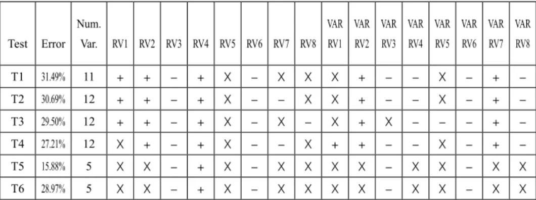
The results of the tests are detailed in tables 8, 9 and 10. In these tables, for each of the tests the following information is provided: the error percentage of the algorithm; the number of variables in the function generated by the algorithm; and, for each variable, the sign of its coefficient in the function (if the variable is not included, this is indicated by the symbol ‘X’).
Test Error Num.
Var. V1 V2 V3 V4 V5 V6 V7 V8
VAR V1 VAR V2 VAR V3 VAR V4 VAR V5 VAR V6 VAR V7 VAR V8
T1 30.84% 11 X + − + X − − X X + − − X − + −
T2 30.02% 13 + + − + − − − X X + − − X − + −
T3 35.73% 2 X X X X X − X X X X X X X − X X
T4 27.82% 9 + + − + X − X X X + X − X − + X
T5 17.99% 3 X X − X X − X X X X X X X − X X
T6 29.60% 3 X X − X X − X X X X X X X − X X
Table 8 Results of the tests for LACE and RFE algorithms and the ‘absolute’ set of variables
Test Error Num.
Var. RV1 RV2 RV3 RV4 RV5 RV6 RV7 RV8
VAR RV1 VAR RV2 VAR RV3 VAR RV4 VAR RV5 VAR RV6 VAR RV7 VAR RV8
T1 31.49% 11 + + − + X − X X X + − − X − + −
T2 30.69% 12 + + − + X − − X X + − − X − + −
T3 29.50% 12 + + − + X − X − X + X − − − + −
T4 27.21% 12 X + − + X − − X + + − − X − + −
T5 15.88% 5 X X − + X − X X X X − X X − X X
T6 28.97% 5 X X − + X − X X X X − X X − X X
Test Error Num.
Var. V1 V2 V3 V4 V5 V6 V7 V8
VAR V1 VAR V2 VAR V3 VAR V4 VAR V5 VAR V6 VAR V7 VAR V8
T1 29.96% 23 X + − − + − − X + X X + + − − X
T2 31.70% 8 X X − + X X X X X X X X X X X X
T3 35.76% 2 X X X X X X X X X X X X X X X X
T4 26.72% 13 X X − + X − + X X X X X X − + X
T5 13.77% 14 X + − + X − + X X X − − X − X +
T6 27.27% 14 X + − + X − + X X X − − X − X +
Table 10 Results of the tests for LACE and RFE algorithms and the ‘complete’ set of variables
Test RV1 RV2 RV3 RV4 RV5 RV6 RV7 RV8
VAR RV1 VAR RV2 VAR RV3 VAR RV4 VAR RV5 VAR RV6 VAR RV7 VAR RV8
T1 X + − + X − + X − + − − X − + −
T2 X X − X X − X X X X X − X − + −
T3 X X X X X − X X X X X X X − X X
T4 X + − X X − − X X + X − X X + X
T5 X X − X X − − X + + X X X X X X
T6 X X − X X − − X + + X X X X X X
Table 10 (cont.) Results of the tests for LACE and RFE algorithms and the ‘complete’ set of variables
From the examination of table 8, which contains the results of the tests when the predictors are the ‘absolute’ variables, we can see that the error rates are in all cases lower than that of a naïve prediction system (i.e. systematically predicting that the first selected company will be the most profitable of the two selected for comparison), the success rate of which is 50%. This means that the estimated models have explanatory power.
Regarding the test whose conditions are similar to that of classification models (T5), the error rate is to a large extent lower than those of the other tests. These results are as expected, as comparing firms from the extreme quartiles is an easier task than those involved in the other tests. It is noticeable that when applying C4.5 algorithm to predict the inclusion of the firms in the two groups considered in T5, the error rate is 26.60%, which is substantially higher. An additional drawback is that a classification model such as C4.5 gives poorer information to the financial analyst (as indicated in previous sections, classification systems predict only the inclusion of a firm in a certain group, but do not rank the companies).
It is also noteworthy that when using the function inferred in test T5 for the assessment of the comparisons between the firms of the four quartiles (test T6), the results are very similar to those of tests T1 to T4. This suggests that for the generation of efficient functions it is not necessary to use the whole database, as with a sample made up of the exemplary cases (companies that are very profitable or very unprofitable) a well-behaving function can also be estimated. This finding is very interesting as it provides an adequate strategy to manage very large databases in an efficient way, contributing to save computation time and costs.
Additionally, we must refer to the signs of the coefficients of the variables of the ‘absolute’ set. Taking into account that all the tests are similar in nature, the signs of the coefficients of a certain indicator should be the same in all the tests for which that variable is selected. Otherwise, instability in the signs of the coefficients would prevent the use of the output of the models for economic and financial analysis. For this reason, we must underline that using LACE and RFE algorithms there is no variable whose coefficient shows indications of instability in its sign.
Table 10 contains the results of the tests when all the variables are included in the prediction set. Once more, these results are very similar to those obtained when considering only the ‘absolute’ variables or only the ‘relative’ set. There are only a few differences, which can be summarized in the following points:
a) The error rates show a slight decrement in almost all the tests. Only for tests T2 and T3 do the error rates increase. In our opinion, this improvement is not enough to justify the doubling of the dimension of the problem (from 16 to 32 indicators).
b) There is a certain instability in the signs of the coefficients (18.75% of the variables). This, as well as the aforementioned drastic increase in the dimension of the problem, make the use of sets of variables constructed in this way inadvisable for economic and financial analysis.
6. SUMMARY AND CONCLUSIONS
In recent years, researchers in the field of Artificial Intelligence have developed algorithms to forecast if a certain individual/entity will have a higher level of a continuous variable in the future than another certain individual/entity, on the basis of a set of indicators. This approach, namely, preference learning, is based in comparisons. It has a key advantage for economic and financial analysts, as it produces rankings of firms, which are very useful in investment decisions.
In a certain way, this method can be considered as something intermediate between regression and classification models, as the information output is richer than that of classification models, which only predict the inclusion of the firm in one out of a limited number of categories, but the input information does not have to be as exact as in regression models, where the researcher has to establish the functional form of the relationship between the variables. So, it is suitable for a problem such as profitability analysis, where neither classification techniques nor regression models have produced good results.
of medium-sized Spanish companies, on the basis of a set of financial indicators. A number of tests have been carried out which try to model the conditions that financial analysts have to deal with. In addition, some other tests replicate the conditions of prior research on business profitability that used classification techniques.
The results obtained are quite satisfactory. The combination of LACE and RFE provides the analyst much more valuable information than a classification approach, such as those inherent to discriminant analysis, logistic regression, classifier neural networks or rule induction systems. It is also noticeable that the model performs quite well when it is made to compare firms from the same branch of activity, no matter which sectoral classification is used.
Another interesting finding is that for the estimation of the functions, the use of the whole sample seems to be unnecessary. For example, for a sample with only the benchmark cases (very profitable or very unprofitable firms), models can be constructed that perform as well as those estimated from the whole sample. Also inadvisable or unnecessary is the use of a high number of variables, as with the reduced sets good results are also obtained, saving computational costs. Finally, and regarding the specification of the financial variables, we must underline that the best results are obtained using the ‘absolute’ form.
7. REFERENCES
ALTMAN, E.I.; HALDEMAN, R.G.; NARAYANAN, P. (1977): “ZETA analysis: a New Model to Identify Bankruptcy Risk of Corporations”, Journal of Banking & Finance, n. 1: 29-54.
BENGIO, Y.; CHAPADOS, N. (2003): “Extensions to Metric-Based Model Selection”, Journal of Machine Learning Research, n. 3: 1209-1227.
BRANTING, K. (1999): “Active Exploration in Instance-Based Preference Modelling”, Paper presented at the Third International Conference on Case-Based Reasoning (ICCBR-99), Monastery Seeon, Germany.
BRANTING, K.; BROOS, P. (1997): “Automated Acquisition of User Preferences”,
BRIEF, R.P.; LAWSON, R.A. (1992): “The Role of the Accounting Rate of Return in Financial Statement Analysis”, Accounting Review, vol. 67, n. 2: 411-426.
CHAGANTI, R.; CHAGANTI, R. (1983): “A Profile of Profitable and Not-So-Profitable Small Businesses”, Journal of Small Business Management, July: 43-51.
COHEN, W.W.; SHAPIRE, R.E.; SINGER, Y. (1999): “Learning to Order Things”,
Journal of Artificial Intelligence Research, n. 10: 243-270.
DE ANDRÉS, J. (2001): “Statistical Techniques vs. SEE5 Algorithm. An Application to a Small Business Environment”, International Journal of Digital
Accounting Research, vol. 1, n. 2: 153-178.
DE ANDRÉS, J.; LORCA, P.; COMBARRO, E.F. (2002): “The Sensitivity of Machine Learning Techniques to Variations in Sample Size: a Comparative Analysis”, International Journal of Digital Accounting Research, vol. 2, n. 4: 131-156.
DE ANDRÉS, J.; LANDAJO, M.; LORCA, P. (2003): Forecasting Business Efficiency by Using Classification Techniques: a Comparative Analysis Based on
a Spanish Case. Social Sciences Research Network. www.ssrn.com.
DE ANDRÉS, J.; LANDAJO, M.; LORCA, P. (2004): “Forecasting Business Profitability by Using Classification Techniques: a Comparative Analysis Based on a Spanish Case”, European Journal of Operational Research, forthcoming.
DÍEZ, J.; DEL COZ, J.; LUACES, O.; GOYACHE, F.; ALONSO, J.; PEÑA, A.; BAHAMONDE, A. (2002): Learning to Assess from Pair-Wise Comparisons. Proceedings of the 8th Iberoamerican Conference on Artificial Intelligence (IBERAMIA), Seville, Spain. Springer-Verlag: 481-490
EISENBEIS, R.A. (1977) “Pitfalls in the Application of Discriminant Analysis in Business, Finance, and Economics”, Journal of Finance, vol. 32, n. 3: 875-900.
GILLINGHAM, D.W. (1980): “A Comparison Between the Attribute Profiles of Profitable and Unprofitable Companies in the United Kingdom and Canada”, Management International Review, vol. 20, n. 4: 64-73.
GORT, M. (1963): “Analysis of Stability and Change in Market Shares”, Journal of Political Economy, vol. 71, n. 1: 51-63.
GUYON, I.; WESTON, J.; BARNHILL, S.; VAPNIK, V. (2002): “Gene Selection for Cancer Classification Using Support Vector Machines”, Machine Learning, n. 46: 389-422.
HARRIS, M.N. (1976): “Entry and Barriers to Entry”, Industrial Organization Review, n. 3: 165-175.
HASLEM, J.A.; LONGBRAKE, W.A. (1971): “A Discriminant Analysis of Commercial Bank Profitability”, Quarterly Review of Economics & Business, vol. 11, n. 3: 39-46.
HERBRICH, R.; GRAEPEL, T.; OBERMAYER, K. (1999): Support Vector Learning for Ordinal Regression. Proceedings of the Ninth International Conference on Artificial Neural Networks, Edinburgh, UK: 97-102.
IZAN, H.Y. (1984): “Corporate Distress in Australia”, Journal of Banking and Finance, n. 8: 303-320.
JOACHIMS, T. (2002): Optimizing Search Engines Using Clickthrough Data. Proceedings of the ACM Conference on Knowledge Discovery and Data Mining (KDD).
KELLY, G.; TIPPET, M. (1991): “Economic and Accounting Rates of Return: a Statistical Model”, Accounting & Business Research, vol. 21, n. 4: 321-329.
KOSKO, B. (1992): Neural Networks and Fuzzy Systems. A Dynamical Systems Approach to Machine Intelligence. Prentice-Hall. Englewood Cliffs, New Jersey, USA.
MARKHAM, I.S.; MATHIEU, R.G.; WRAY, B.A. (2000): “Kanban Setting through Artificial Intelligence: a Comparative Study of Artificial Neural Networks and Decision Trees”, Integrated Manufacturing Systems, vol. 11, n. 4: 239-259.
MARTIN, D. (1977): “Early Warning of Bank Failure: a Logit Regression Approach”, Journal of Banking & Finance, n. 1: 249-276.
MURTHY, S. K.; KASIF, S.; SALZBERG, S. (1994): “A System for Induction of Oblique Decision Trees”, Journal of Artificial Intelligence Research, n. 2: 1-32.
PLATT, H.D.; PLATT, M.B. (1990): “Development of a Class of Stable Predictive Variables: the Case of Bankruptcy Prediction”, Journal of Business Finance and Accounting, vol. 17, n. 1: 31-51.
RAKOTOMAMONJY, A. (2003): “Variable Selection Using SVM-Based Criteria”, Journal of Machine Learning Research, n. 3: 1357-1370.
SHIPCHANDLER, Z.H.; MOORE, J.S. (2000): “Factors Influencing Foreign Firm Performance in the US Market”, American Business Review, vol. 18, n. 1: 62-69.
SCHUURMAANS, D.; SOUTHEY, F. (2002): “Metric-Based Methods for Adaptive Model Selection and Regularization”, Machine Learning, n. 48: 51-84.
SCHUURMANS, D. (1997): A New Metric-Based Approach to Model Selection. Proceedings of the AAAI/IAAI: 552-558.
TESAURO, G. (1989): Connectionist Learning of Expert Preferences by Comparison Training. Advances in Neural Information Processing Systems, Proceedings of the NIPS’88. MIT Press, Massachussets, USA: 99-106.
TSAI, C.Y. (2000): “An Iterative Feature Reduction Algorithm for Probabilistic Neural Networks”, Omega, n. 28: 513-524.
UTGOFF, P.; SAXENA, S. (1987): Learning a Preference Predicate. Proceedings of the Fourth International Workshop on Machine Learning. Morgan Kaufmann. Irvine, California, USA: 115-121.
WALTER, J.E. (1959): “A Discriminant Function for Earnings-Price Ratios of Large Industrial Corporations”, Review of Economics & Statistics, n. 41: 44-52.
WATSON, C.J. (1990): “Multivariate Distributional Properties, Outliers, and Transformation of Financial Ratios”, Accounting Review, vol. 65, n. 3, July: 662-695.
WEIR, C. (1996): “Internal Organization and Firm Performance: an Analysis of Large UK Firms under Conditions of Economic Uncertainty”, Applied Economics, vol. 28, n. 4: 473-481.