Transport and Telecommunication, 2014, volume 15, no. 2, 130–143
Transport and Telecommunication Institute, Lomonosova 1, Riga, LV-1019, Latvia DOI 10.2478/ttj-2014-0012
HOMOGENIZATION EFFECTS OF VARIABLE SPEED LIMITS
Alvaro Garcia-Castro, Andres Monzon
Transportation Research Centre (TRANSyT) Universidad Politecnica de Madrid.
Escuela de Ingenieros de Caminos, Canales y Puertos, Avda. Profesor Aranguren s/n. Madrid. Spain Phone: +34 91 336 52 34. Fax: +34 91 336 53 62. E-mail: [email protected]
Changing factors (mainly traffic intensity and weather conditions) affecting road conditions require a suitable optimal speed at any time. To solve this problem, variable speed limit systems (VSL) – as opposed to fixed limits – have been developed in recent decades. This term has included a number of speed management systems, most notably dynamic speed limits (DSL).
In order to avoid the indiscriminate use of both terms in the literature, this paper proposes a simple classification and offers a review of some experiences, how their effects are evaluated and their results
This study also presents a key indicator which measures the speed homogeneity and a methodology to obtain the data based on floating cars and GPS technology applying it to a case study on a section of the M30 urban motorway in Madrid (Spain). It also presents the relation between this indicator and road performance and emissions values.
Keywords: Effectiveness indicator, variable speed limits, dynamic speed limits, GPS application, speed management, floating car data
1. Introduction
The main tool used by authorities to manage speed is the setting of speed limits, which tend to be fixed. However, the optimal speed cannot remain constant at all times, as the road conditions are affected by numerous factors, mainly traffic intensity and weather conditions (Giles, 2004).
Speed can be regarded as a key factor that directly affects certain aspects of the road such as traffic performance, road safety and environmental externalities.
1) Traffic performance
Together with intensity and density, speed is one of the key factors determining road capacity. At a critical speed and the corresponding critical intensity or density, the state of flow will change from stable to unstable and, speed differences and braking process can therefore lead to congestion and reduced road capacity (Van Nes & etc., 2008).
2) Road safety
It is generally accepted that high speeds involve a high risk to road safety. This idea is supported by a large number of studies which highlight the relationship between speed and road safety. For instance, ref. (Elvik, 2005) shows an extensive review of 98 studies containing 460 estimates of the relationship between changes in speed and changes in the number of accidents or accident victims, concluding “the relationship between speed and road safety is causal, not just statistical”.
3) Environmental externalities
Apart from vehicle technologies, speed is a very important factor determining negative environmental effects such as CO2 emissions, pollutants (Ntziachristos & Samaras, 2000) and noise
(Makarewicz & Gałuszka, 2011).
The concern of traffic authorities to adapt traffic speed to changing road conditions has led in recent decades to the development of variable speed limits (VSL).
2. Variable Speed Limits. Classification
VSL is a broad term that includes many speed management systems with different motivations and control algorithms. VSL can be defined simply as speed limit management systems, which are time dependant. Some authors confine the term VSL to systems which utilize traffic detectors to determine the appropriate speed (Sisiopiku, 2011); however, this fails to take into account the existence of VSL, which operate following prefixed calendars or timetables based on historical data. It is thus necessary to classify VSL as follows:
2.1. Scheduled Variable Speed Limits (SVSL)
Seasonal Variable Speed Limits
These are applied to a specific type of road and set the speed limit during a particular season, with the most common being the winter/summer speed limits.
An example can be found in the Nordic countries due to their extreme weather conditions during the winter months. In Finland the reason for lowering winter speed limits is primarily the adverse road and driving conditions (Peltola, 2000).
Experiments involving the setting of seasonal speed limits for safety reasons can be also found in the northern states of the U.S.A. For instance, the Wyoming Department of Transport first implemented the seasonal speed limit for six months beginning on October 15, 2008 (Wyoming Department of Transport, 2012).
In the Austrian region of Tyrol during the winter of 2006/2007, the speed limit was temporarily reduced on the Inn Valley Motorway from 130 km/h to 100 km/h, mainly due to high levels of air pollution during previous winter seasons (Land Tirol, 2012).
Hourly Variable Speed Limits
These are mainly applied to prevent or reduce certain negative externalities in a specific road section or street at particular times.
Experiments of this type can be found in some German or American cities where authorities have implemented VSL in school areas in order to reduce speed when schools are open or at exactly the times children are arriving or leaving (Lehming, 2008), (Transport and Main Roads, 2011).
There are also experiments related to noise reduction during night hours in residential areas or close to hospitals and other facilities. In the city of Berlin (Lehming, 2008), speed is limited during the night hours to 30 km/h in residential or mixed areas.
Figure. 1. Proposed classification of Variable Speed Limits
2.2. Dynamic Speed Limits (DSL)
The term “dynamic” implies a force which produces a change in state or movement. In this case, the “forces” that produce changes in speed limits are the conditions in and around the road. Therefore, Dynamic Speed Limits can be defined as a type of Intelligent Transport System (ITS) which produces changes in speed limits in response to accurate information regarding road, driving, weather and/or environmental conditions (Van Nes & etc., 2008).
Pure manual control methods are based simply on a protocol that the operators activate when one or more levels (traffic intensity, visibility, air pollution, etc.) exceed the pre-set thresholds.
The concept of automatic DSL is based on various approaches, ranging from basic protocols according to particular thresholds (similar to manual methods) to complex algorithms based on multi-objective optimization, game theory, predictive control and genetic algorithms (Hegyi & etc., 2005; Xu & etc., 2006; Ghods & etc., 2010; Xiao-Yun & etc., 2010).
3. Evaluation of Variable Speed Limits
DSL are being implemented worldwide; however their effects are not yet clearly defined, and in some cases their benefit is not fully proven.
Based on international experiments and research studies, we summarize the way in which DSL affect the parameters of traffic performance, road safety and environmental levels, and the variables that are used to assess their effectiveness.
3.1. Traffic Performance
With regard to traffic performance and traffic flow behaviour, there are several parameters which may be affected by the implementation of DSL, including particularly speed and capacity.
The reduction in average speed and speed variations depends largely on the type of speed limits imposed (mandatory or recommended) and their enforcement. Most DSL operate as mandatory limits, such as the M25 controlled motorway around London (Highways Agency, 2004), although there are also some systems with recommended speed limits, such as the Motorway Control System (MCS) on the E4 in Stockholm (Nissan & Bang, 2006).
These systems are based on the capacity increase that occurs when speed and speed variations are reduced by high flow levels. Moreover, speed homogenization reduces the number of acceleration and deceleration manoeuvres and therefore the oscillations in traffic flow (García, 2009). Ref. (Heydecker & Addison, 2011) shows that under certain congestion conditions, speed determines density; based on this observation, the relationship between density and speed can be estimated depending on speed limits.
The reduction of speed limits has a considerable effect on the speed differential between lanes. In (Van Nes & etc., 2008), the conclusions show that it can be said that dynamic speed limit systems do increase the homogeneity of the driving speed.
Based on computer simulators, some authors evaluate positively the effects of DSL on traffic performance. Reference (Zhicai & etc., 2004) shows the simulation of a number of types of DSL scenarios, and the results indicate that the benefits of DSL are obvious when the traffic volume is equal to or greater than 2,800 veh. in a double-lane freeway. Ref. (Hegyi & etc., 2005) simulates the effects of DSL on the prevention of congestion caused by shockwaves, obtaining a reduction in total travel time of 21.7%.
Germany has a long tradition of implementing VSL, and in particular DSL. The first experiment was implemented in 1965 on the A8 motorway between Munich and Salzburg, with good results in terms of harmonization and reduction of speed differences between lanes. These results and many others from German motorways can be found in (Schick, 2003). Among these cases, we can highlight the report on the A5 motorway in Frankfurt. Based on data from video recording and induction loops, the authors found a significant increase in the empirical maximum traffic intensity in the southbound direction from 5,200 veh/h. to 5,900 veh/h. (about a 10% increase). However other studies in the Netherlands (Hoogendoorn, 1999) estimate the capacity increase at around 2%.
The M25 in the U.K. can also be highlighted as a successful implementation of DSL. During the first year of operation, a section of this controlled motorway absorbed a 1.5% increase in throughput over 5-hour peak periods, without any detectable increase in congestion levels. Traffic conditions have improved as a result of the reduction in frequency and severity of shockwaves. The study (Highways Agency, 2004) revealed a reduction of over 25% in the typical number of shockwaves during the morning peak period. It has also been observed that the traffic is now more evenly spread across all four lanes.
Reference (Nissan & Bang, 2006) studied the application of DSL on the E4 motorway through Stockholm, revealing that lane changes were reduced by over 50%, and that lane distribution became more balanced after the implementation. However, this phenomenon can have negative effects in sections with a high density of on-ramps, as this will lead to smaller gaps in the traffic on the outside lane, making the merging process more difficult and therefore creating congestion on the on-ramp (Knoop & etc., 2010).
DSL. In the southbound corridor, the use of progressively slower speed limits depending on traffic volume has reduced congestion by between 16% and 40%, depending on the section (ECMT, 2007).
3.2. Road Safety
The effects mentioned in the previous section can also have a positive impact on road safety, as decreases in the speed limits can lead to a reduction in the speed differences between successive vehicles, resulting in a decline in rear-end collisions.
Reference (Lee & etc., 2007) presents a simulation-based study showing the potential safety benefits of DSL using a real-time crash prediction model integrated with a microscopic traffic simulation model. The study found that dynamic speed limits can reduce average total crash potential by approximately 25%, by temporarily reducing speed limits during hazardous traffic conditions. Positive effects of DSL have also been found in other simulation-based studies, such as (Piao & McDonald, 2008).
Regarding the study of the DSL implemented, an analysis of crash data in Germany has shown that the use of dynamic speed limit and speed warning signs reduced the crash rate by 20 to 30% (Robinson, 2000). Other German studies cited by (Schick, 2003) estimate a reduction in the number of accidents of over 30% (A5 motorway, near Frankfurt), and a similar decline in fatalities by more than 60%. In Stuttgart, the reduction in accidents caused by fog conditions is as high as 86%.
In the UK (Highways Agency, 2004) data are analysed from the M25 in order to compare them with the trends. The impact of introducing the controlled motorway driving environment (mainly DSL and managed lanes) has been an estimated reduction in injury accidents of 10% during the period of operation, and a decrease in the ratio of damage of 20%.
The aforementioned programme in the South of France also had very positive road safety results, with crashes reduced by 10–20% (ECMT, 2007).
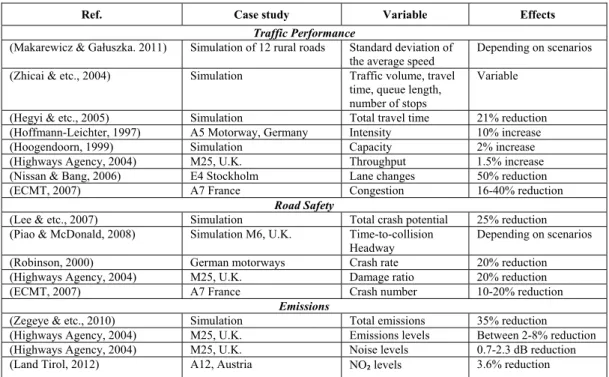
Table 1.Summary of evaluation variables used in different research studies
Ref. Case study Variable Effects
Traffic Performance
(Makarewicz & Gałuszka. 2011) Simulation of 12 rural roads Standard deviation of the average speed
Depending on scenarios
(Zhicai & etc., 2004) Simulation Traffic volume, travel time, queue length, number of stops
Variable
(Hegyi & etc., 2005) Simulation Total travel time 21% reduction (Hoffmann-Leichter, 1997) A5 Motorway, Germany Intensity 10% increase
(Hoogendoorn, 1999) Simulation Capacity 2% increase
(Highways Agency, 2004) M25, U.K. Throughput 1.5% increase
(Nissan & Bang, 2006) E4 Stockholm Lane changes 50% reduction
(ECMT, 2007) A7 France Congestion 16-40% reduction
Road Safety
(Lee & etc., 2007) Simulation Total crash potential 25% reduction (Piao & McDonald, 2008) Simulation M6, U.K. Time-to-collision
Headway
Depending on scenarios
(Robinson, 2000) German motorways Crash rate 20% reduction
(Highways Agency, 2004) M25, U.K. Damage ratio 20% reduction
(ECMT, 2007) A7 France Crash number 10-20% reduction
Emissions
(Zegeye & etc., 2010) Simulation Total emissions 35% reduction
(Highways Agency, 2004) M25, U.K. Emissions levels Between 2-8% reduction (Highways Agency, 2004) M25, U.K. Noise levels 0.7-2.3 dB reduction
(Land Tirol, 2012) A12, Austria NO₂ levels 3.6% reduction
3.3. Environmental effects
It is well-known that improved traffic flows can have a significant impact on emission levels (Benedekand & Rilett, 1998). There are very few approaches based on simulating emissions in DSL. Of particular note is the simulation of a case study based on model predictive control, where the total emissions are reduced by over 35% (Zegeye & etc., 2010).
between Junction 15 and 16. The reduction in stop-start driving and the improved compliance with the speed limits have reduced the weekday traffic noise adjacent to the motorway by around 0.7 decibels, with reductions at some points of up to 2.3 dB.
Another example can be found in Inn Valley in Austria. The effects of the implementation of DSL were analysed on this motorway after one year of operation (November 2007 to November 2008). In a before/after evaluation the results show that NO2 emissions were reduced by 3.6%. Also, the NO2 limit value for short-term exposure (half-hour limit: 200 g/m³) was exceeded only twice during the first year of operation, while without the DSL in operation, it is estimated that it would have been exceeded nine times (Land Tirol, 2012).
4. Methodology to Evaluate VSL Systems Using an Aggregate Effectiveness Indicator
4.1. Effectiveness indicator. Definition
Table 1 shows the large number of variables which are used in the scientific literature and other public reports to evaluate the effects of DSL. This fact highlights the need to find a single variable which makes possible to evaluate the system’s effectiveness easily and concisely by aggregating the potential effects on traffic performance, road safety and emissions.
With regard to traffic performance, several of the aforementioned studies point out that the homogenization of speed (i.e., lower acceleration rates) contributes to a smooth traffic flow (García, 2009), an increase in capacity (Heydecker & Addison, 2011) and the attenuation of shockwaves (Hegyi & etc., 2005).
Likewise, road safety has been proven to be related with traffic and speed homogeneity (Van Nes & etc., 2008), (Piao & McDonald, 2008), (Fildes & Lee, 1993), (Wegman & etc., 2008). It can therefore be concluded that there is a clear relation between speed variations and number of accidents.
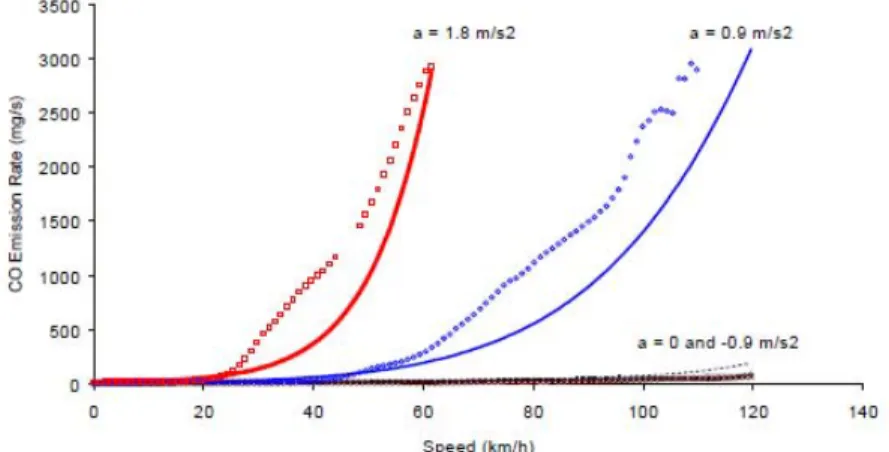
Figure. 2. Regression fit for CO emissions as a function of speed and acceleration rates. Source (Rakha & etc., 2000)
Many research studies (Rakha & etc., 2000; El-Shawarby & etc., 2005; Joumard & etc., 1995; Ding & Rakha, 2002) also state that, apart from mean or average speed, positive acceleration rates also have a major impact on emissions, as shown on Figure 2 from (Rakha & etc., 2000).
It has thus been possible to pinpoint instant acceleration as a key factor by evaluating the effectiveness of implementing DSL, and then proposing an aggregate indicator as follows:
Positive Accumulated Acceleration (PAA) is defined as the sum of the speed variations on a particular road section.
Mathematically, it is the cumulative integral of the positive acceleration law (1).
( )
(
)
t t t t
t t 1
t t t 1
0 0 0
0
α (V V )
PAA a t dt a Δt Δt α V V .
Δt
+ + −
−
⋅ −
=
∫
≅∑
⋅ =∑
⋅ =∑
⋅ −If
(
V
t−
V
t−1) 0
>
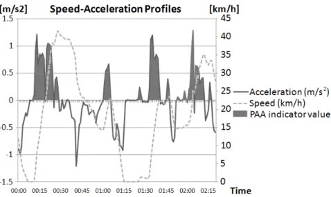
then α = 1 (1)Graphically, PAA is the positive area of the region bounded by the acceleration law, as shown on Figure 3.
Figure 3. Graphic representation of PAA indicator from an acceleration function
The PAA indicator makes it possible to compare the same section before and after the implementation of DSL, thus evaluating its effectiveness.
4.2. Data collection and evaluation
As already mentioned, the PAA indicator is simply based on speed variations, and the data required to calculate it is relatively easy to obtain.
Speed data are often collected by induction loops located at certain points on the road, but this method makes it impossible to establish the speed evolution between two loops, and leads to the possibility of distorted results.
It is thus essential to obtain speed data at short time intervals, and the methodology proposed is therefore based on GPS technologies. With a small portable device it is very simple to collect and download speed data, position and so on every second, which allows a very accurate speed profile to be obtained along the road section analyzed.
The methodology is based on a before & after evaluation, by observing the evolution of the PAA indicator. Ideally, the number of trip repetitions should be fairly high in order to limit variations caused by other factors such as meteorology, extraordinary events, incidents, etc. In any case, the trips must be made in the same time slot and on days with similar behaviour in terms of traffic. In the event of a limited sample, particular care must be taken to ensure that the conditions are almost the same. The traffic intensity upstream must be guaranteed to be substantially the same when performing the before & after trips.
Once the valid data has been processed and selected, the implementation of DSL can be valued positively if the indicator PAAa (activated) is lower than PAAd (deactivated).
5. Pilot Test Case: West Section of Madrid M30 Motorway
5.1. Description
Madrid is a city of about 3.5 million inhabitants, and up to 6 million in its metropolitan area. The city is surrounded by three motorway ring-roads, with the M30 the closest to the city centre.
In the afternoon peak hours on a normal working day, the M30 has high traffic levels southbound on its east and west sections. In an attempt to avoid this habitual congestion and its externalities, the Madrid Traffic Department is testing a DSL system based on recommended speed limits.
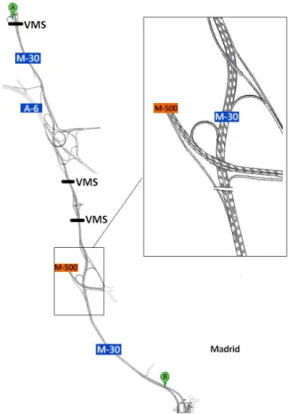
The DSL system consists of three Variable Message Signs (VMS) situated before the M500 junction. These VMS display a recommended speed limit of 40, 60 or 80 km/h, depending on the control algorithm. This is based on instant speed and traffic intensity data recorded by induction loops situated along the section.
Figure 4. West Madrid motorway ring-road and the 5.8 km. test section (from A to B) with the location of the Variable Message Signs (VMS). The bottleneck junction where the congestion usually starts (M-500) is highlighted
A microscopic car study was undertaken in the afternoon peak traffic period between 18:00-20:00. A total of nine trips were made on the 6th and 7th June (Tuesday and Wednesday) with the DSL system
activated. One week later (12th and 13th June) another nine trips were performed at exactly the same
times, this time with the DSL system deactivated. The intensity levels upstream for the test days were very similar, with a maximum deviation of 2.63% from the mean value (Table 2). The weather was sunny and there were no particular incidents or accidents during the test trips, except for unusual congestion on 6 June, which caused the system not to be automatically activated.
Table 2. Traffic flow intensities upstream (Measuring point PM 22421)
Time
Date
Mean
Max. mean deviation
05-June
06-June
12-June
13-June
18:00 3159 3196 3114 3324 3198 -2.63% 19:00 3501 3544 3506 3440 3498 -1.65%
The mobile study was carried out using an instrumented vehicle (Skoda Fabia TDI) equipped with a GPS data recorder (747+ GPS Trip Recorder), which was subsequently downloaded as an Excel Sheet (.csv) and georeferenced (.kml) documents.
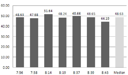
Likewise, seven trips (Figure 5) in free flow (southbound mornings) were performed in order to study the variability of the PAA in similar conditions and to isolate the effects of DSL from any other which may influence the results (small disturbances and changes in driving style).
Figure 5. PAA indicator values in free flow. Obtained in the morning hours of the 5th and 6th June
From this analysis, it can be concluded that in free flow and in similar conditions, 99% (confidence level = 0.99, ά = 0.01) of the PAA results present a deviation from the median of less than 2.19 (confidence limits). Therefore any deviation greater than this value will be assigned to the effects of DSL.
5.1. Analysis of results
5.1.1. Effects on speed homogenization
Table 3 shows the resulting values of the PAAa and PAAd from the trips performed on the 5th and
12th June. The results on Wednesday 6 are considered invalid, as the system was automatically
disconnected due to the unusual and extreme congestion (recorded speed under the operation thresholds). Table 3. Values obtained for PAA Effectiveness indicator. Congested trips
Activated Deactivated Tuesday 5 and 12. Afternoon peak
Time PAA values Time PAA values
18:30 91.68 18:29 92.04 18:52 88.20 18:52 88.89 19:11 72.23 19:10 90.99 19:32 59.62 19:32 105.88 19:51 63.54 19:55 69.36
Average 75.05 Average 89.43
Wednesday 6 and 13. Afternoon peak
18:28 125.84 18:27 99.20
18:50 124.06 18:49 86.62
19:14 130.74 19:13 90.68
19:38 73.21 19:38 76.82
Average 113.46 Average 88.33
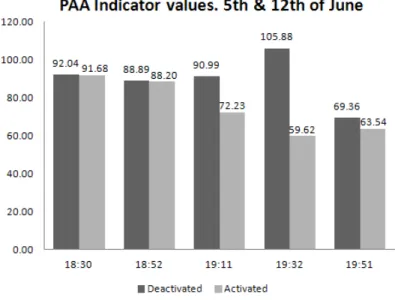
Figure 6. Comparison of the effectiveness indicator (PAA) on Tuesday 5th and 12th June
Figure 6 shows that PAAa and PAAd values are fairly similar, except for the trips that are highly affected by congestion. An analysis of the speed profiles on Figure 7 and the indicator values shows that in the 19:11 trip, the speed distribution is more homogeneous, although the congestion levels are similar. This fact causes the congestion on the following trip (19:32) to remain at similar levels (or even to decrease) while DSL is activated, and the queue length to increase while deactivated.
Figure 7. Comparison of speed profiles for trips with DSL activated and deactivated
5.1.2. Effects on traffic performance
Table 4 shows the relation (in percentage) between traffic throughput downstream and upstream during the peak hours in the test days.
Table 4. Traffic throughput relation downstream/upstream the test section
Date 05-June 06-June 07-June 12-June 13-June 14-June Mean
Activated 183% 181% 178% - - - 181%
Deactivated - - - 181% 177% 178% 179%
The results show a slight improvement of 2% in the relation between the traffic flow downstream and upstream during the test days.
Table 5 shows the travel times during peak hour trips on the 5th and 12th June. The results on
Wednesday 6 are considered invalid, as the system was automatically disconnected due to the unusual and extreme congestion (recorded speed under the operation thresholds).
Table 5.Trip travel time per day (activated/deactivated)
Activated Deactivated Tuesday 5 and 12. Afternoon peak
Time Travel time Time Travel time
18:30 7:59:00 18:29 6:59:00
18:52 7:28:00 18:52 6:15:00
19:11 6:35:00 19:10 6:10:00
19:32 5:36:00 19:32 7:24:00
19:51 4:45:00 19:55 4:46:00
Average 6:28:00 Average 6:18:00 Wednesday 6 and 13. Afternoon peak
18:28 9:34:00 18:27 7:21:00
18:50 10:13:00 18:49 6:32:00
19:14 10:29:00 19:13 6:56:00
19:38 7:02:00 19:38 6:04:00
Average 9:19:00 Average 6:43:00
Rejecting the results of the 6th June and comparing similar trips of activated and deactivated days,
the result shows a 3% increase in travel time with the system activated.
From the traffic performance point of view, the results are contradictory. Firstly, the application of variable speed limits produces in this case a slight improvement in the throughput relation between traffic flow downstream and upstream the controlled section. On the other hand, travel time suffers a small penalty, which is related with the more restrictive speed limits.
However, it is important to mention that although this travel time increase, PAA values decrease when the system is activated. This means that the system achieves more homogeneous speed profiles for the same travel times (Figure 8).
5.1.3. Environmental effects
Together with road safety considerations, positive environmental effects are one of the main reasons for implementing variable speed limits systems in motorways. Most of the studies reviewed show positive results in case of emissions and fuel consumptions.
In the presented case study, reductions of PAA values, which mean more homogeneity in speed profiles, imply reductions in emissions and fuel consumption. This reduction can be quantified by introducing the speed profiles in micro emissions models, such as VERSIT+ (Smit & etc., 2007).
The output of the VERSIT+ model for the presented case study is summarized in Table 6. Table 6. Trip travel time per day (activated/deactivated)
Activated Deactivated
Tuesday 5 and 12. Afternoon peak
Time CO2 NOx PM10 Time CO2 NOx PM10
18:30 1021 1.880 0.2396 18:30 1040 1.994 0.2413
18:52 1037 1.985 0.2481 18:52 1058 2.103 0.2462
19:11 973.1 1.845 0.2173 19:11 1074 2.379 0.2387
19:32 961.6 1.845 0.2216 19:32 1102 2.226 0.2495
19:51 1014 2.209 0.2199 19:51 1034 2.303 0.2200
Average 1001.3 1.952 0.2293 Average 1061.6 2.201 0.2391
Wednesday 6 and 13. Afternoon peak
Time CO2 NOx PM10 Time CO2 NOx PM10
18:28 1148 2.197 0.2704 18:27 1079 2.028 0.2523 18:50 1171 2.333 0.2819 18:49 1047 2.206 0.2426 19:14 1165 2.133 0.2703 19:13 1051 2.037 0.2431 19:38 1002 1.802 0.2442 19:38 1023 1.958 0.2380
Average 1121.5 2.116 0.2667 Average 1050 2.057 0.2440
As in previous analysis, rejecting the extreme results of the 6th June, the emissions savings are
shown on Table 7.
Table 7. Emissions savings comparing the scenarios activated vs. deactivated.
Emissions CO2 NOX PM10
Savings 2.58% 4.14% 2.54%
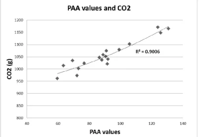
Analysing the relation between Positive Accumulated Acceleration indicator and the emissions, both CO2 and the pollutants show the same tendency. Despite this tendency is clear, NOxis not clearly
correlated with the indicator, obtaining a low value of R2. Figure 9, 10 and 11 show the relation between
PAA and CO2, NOx and PM10 respectively.
Figure 10. PAA values and NOx emissions
Figure 11. PAA values and PM10 emissions
6. Conclusions
After classifying Variable Speed Limits, the literature review has shown that in many cases VSL (and in particular VSL based on dynamic control) have been beneficial in terms of traffic performance, road safety and environmental effects. Based on the accumulated acceleration in a section (or instantaneous speed variations) the methodology described provides a single indicator (PAA) to evaluate whether the implementation of VSL is working properly and has the potential to produce the desired effects.
To evaluate the feasibility of the methodology on a practical level, a pilot study was carried out on a stretch of the M30 motorway ring-road in Madrid. This demonstrated the defined PAA effectiveness indicator to be specific, measurable, reliable and traceable.
Once the effects of driving variability have been statistically bounded by analyzing the trips in free flow, the variability in traffic intensities requires a greater number of routes. Regarding the traffic performance, traffic data extracted from induction loops shows an increasing traffic throughput when the system is activated, slightly penalising travel times.
Although it has been not possible to cross the obtained data with road safety figures, in general it can be concluded that the homogenization achieved by the implementation of variable speed limits systems has positive effects.
Future research in relation to this indicator could be directed towards establishing more solid quantitative relationships between changes in the value of the PAA effectiveness indicator and the VSL effects, especially regarding road safety.
Acknowledgments
This work was supported in part by the European Commission, under the project ICT-EMISSIONS, “Development of a Methodology and Tool to Evaluate the Impact of ICT Measures on Road Transport Emissions”, Grant agreement no: 288568.
References
1. Giles, M.J. (2004). Driver speed compliance in Western Australia: a multivariate analysis. Transport Policy, 11(3), 227–235.
2. Van Nes, N., Brandenburg, S. & D. Twisk. (2008). Dynamic speed limits; effects on homogeneity of driving speed. Intelligent Vehicles Symposium, IEEE, 269.
3. Elvik, R. (2005). Speed and road safety – Synthesis of evidence from evaluation studies, Transportation Research Record: Statistical Methods; Highway Safety Data, Analysis, and Evaluation; Occupant Protection; Systematic Reviews and Meta-Analysis, no. 1908 (pp. 59–69). Washington.
4. Ntziachristos, L. & Z. Samaras. (2000). Speed-dependent representative emission factors for catalyst passenger cars and influencing parameters. Atmospheric Environment, 34(27), 4611–4619.
5. Makarewicz, R. & M. Gałuszka. (2011). Road traffic noise prediction based on speed-flow diagram. Applied Acoustics, 72(4), 190–195.
6. Sisiopiku, V. (2011). Variable Speed Control: Technologies and Practice, Proceedings of the 11th
Annual Meeting of ITS America, 2011, Virginia.
7. Peltola, H. (2000). Seasonally changing speed limits – Effects on speeds and accidents. Transportation Research Record: Journal of the Transportation Research Board, 1734, 46–51. 8. Wyoming Department of Transport. (May 10, 2012). Variable speed limits replaces seasonal limit
on I-80 section, 2010. Available at –
http://www.dot.state.wy.us/wydot/news_info/news_releases;jsessionid=8C31A2CE4E803278FC9A 1703A8425BC4?template=tpl.newsDetail&newsID=910
9. Land Tirol. (May 24, 2012). Tempo 100 auf der Autobahn – warum? (In German). Available at – http://www.tirol.gv.at/themen/verkehr/verkehrsplanung/verkehrsprojekte/tempo100
10. Lehming, B. (2008). Noise reduction plan for Berlin – Action plan, Senatsverwaltung für Gesundheit, Umwelt und Verbraucherschutz. Abt. III Umweltpolitik, Referat Immissions schutz. Berlin.
11. Transport and Main Roads. (2011). School Environment Safety Technical Guidelines. Queensland Government, Queensland, Australia.
12. Allaby, P., Hellinga, B. & M. Bullock. (2007). Variable Speed Limits: Safety and Operational Impacts of a Candidate Control Strategy for Freeway Applications. Intelligent Transportation Systems, IEEE Transactions on, 8(4), 671–680.
13. Hegyi, A., De Schutter, B. & J. Hellendoorn. (2005). Optimal coordination of variable speed limits to suppress shock waves. IEEE Transactions on Intelligent Transportation Systems, 6(1), 102–112. 14. Xu, J., Liang, F. & W. Yu. (2006). Coordinated Control of Variable Speed Limits Based on Neural
Dynamic Optimization. In “Vehicular Electronics and Safety”, ICVES, IEEE International Conference on Vehicular Electronics and Safety (pp. 163). Shanghai, China.
15. Ghods, A.H., Fu, L. & A. Rahimi-Kian. (2010). An Efficient Optimization Approach to Real-Time Coordinated and Integrated Freeway Traffic Control. IEEE Transactions on Intelligent Transportation Systems, 11(4), 873–884.
16. Xiao-Yun, L., Varaiya, P., Horowitz, R., Dongyan, S. & S.E.Shladover. (2010). A new approach for combined freeway Variable Speed Limits and Coordinated Ramp Metering. In Proceedings of the 13th International IEEE Conference on Intelligent Transportation Systems (pp. 491). Funchal,
17. Highways Agency. (2004). M25 Controlled Motorways. Summary Report. Bristol (UK): Highways Agency Publications Group.
18. Nissan, A. & X. Bang. (2006). Evaluation of impacts of the motorway control system (MCS) in Stockholm. In Proceedings ofthe European Transport Conference, AET. Strasbourg, France. 19. García, A. (2009). Estudio sobre la gestión variable de la velocidad en las vías de acceso a las áreas
urbanas, Cambra Oficial de Comerç, Indústria i Navegació de Barcelona. Barcelona, Spain.
20. Heydecker, B.G. & J.D. Addison. (2011). Analysis and modelling of traffic flow under variable speed limits. Transportation Research, Part C: Emerging Technologies, 19(2), 206–217.
21. Zhicai, J., Xiaoxiong, Z. & Y. Hongwei. (2004). Simulation research and implemented effect analysis of variable speed limits on freeway. In Proc. of the 7th International IEEE Conference on Intelligent Transportation Systems (pp. 894). Washington.
22. Schick, P. (2003). Einfluss von Streckenbee in flussungs anlagen auf die Kapazität von Autobahn abschnittensowie die Stabilität des Verkehrsflusses. (In German) Ph. D. Thesis. Institut für Straßen- und Verkehrswesen Universität, Stuttgart.
23. Hoogendoorn, S.P. (1999). Multiclass continuum modelling of multilane traffic flow. Delft, The Netherlands: Delft University Press.
24. Knoop, V.L., Duret, A., Buisson, C. & B. Van Arem. (2010). Lane distribution of traffic near merging zones influence of variable speed limits. In Proc. of the 13th International IEEE Conference on Intelligent Transportation Systems (ITSC) (pp. 485). Madeira, Portugal.
25. ECMT. (2007). Congestion management measures that release or provide new capacity. In OECD/ECMT (Eds.), Managing urban traffic congestion (pp. 229). France: OECD Publishing. 26. Lee, C., Hellinga, B. & F. Saccomanno. (2007). Assessing safety benefits of variable speed limits.
Transportation research record: journal of the transportation research board, 1897, 183–190. 27. Piao, J. & McDonald, M. (2008). Safety Impacts of Variable Speed Limits – A Simulation Study.
In Proc. of the 11th International IEEE Conference on Intelligent Transportation Systems, (ITSC)
(pp. 833). Beijing, China.
28. Robinson, M. (2000). Examples of Variable Speed Limit Applications. In Speed Management Workshop, the 79th Annual Meeting of Transportation Research Board. Washington.
29. Benedekand, C.M., Rilett, L.R. (1998). Equitable traffic assignment with environmental cost functions. Journal of Transportation Engineering – ASCE, 124, 16–22
30. Zegeye, S.K., De Schutter, B., Hellendoorn, J. & E.A. Breunesse. (2010). Variable speed limits for area-wide reduction of emissions. In Proc. of the 13th International IEEE Intelligent Transportation Systems (ITSC) (pp. 507–510). Funchal, Portugal.
31. Hoffmann-Leichter. (1997). Untersuchung der Auswirkung der Verkehrsbeeinflussungs anlage auf der A5 Freidberg – Frankfurt auf Verkehrsablauf, Verkehrssicherheit und Reisezeit, Hessischen Landesamtes fürStraßen – und Verkehrswesen. Falkensee Germany.
32. Fildes, B.N. & S.J. Lee. (1993). The speed review: Road environment, Behavior, Speed limits, Enforcement and Crashes, (pp. 33–34). Monash University, Accident Research Centre.
33. Wegman,V., Aarts, L. & C. Bax. (2008). Advancing sustainable safety: National road safety outlook for The Netherlands for 2005–2020. Safety Science, 46(2), 323–343.
34. Rakha, H., Van Aerde, M., Ahn, K. & A.A. Trani. (2000). Requirements for evaluating traffic signal control impacts on energy and emissions based on instantaneous speed and acceleration measurements. Transportation Research Record: Journal of the Transportation Research Board, 1738(1), 56–67.
35. El-Shawarby, I., Ahn, K. & H. Rakha. (2005). Comparative field evaluation of vehicle cruise speed and acceleration level impacts on hot stabilized emissions. Transportation Research, Part D: Transport and Environment, 10(1), 13–30.
36. Joumard, R., Jost, P., Hickman, J. & D. Hassel. (1995). Hot passenger car emissions modelling as a function of instantaneous speed and acceleration. Science of the Total Environment, 169(1–3), 167–174.
37. Ding, Y. & H. Rakha. (2002). Trip-based explanatory variables for estimating vehicle fuel consumption and emission rates. Water, Air, & Soil Pollution: Focus, 2(5), 61–77.