The optimal combination: Grammatical swarm, particle swarm optimization
and neural networks
Luis Fernando de Mingo López*, Nuria Gómez Blas, Alberto Arteta
A B S T R A C T
Social behaviour is mainly based on swarm colonies, in which each individual shares its knowledge about the environment with other individuáis to get optimal solutions. Such co-operative model differs from competitive models in the way that individuáis die and are born by combining information of alive ones. This paper presents the particle swarm optimization with differential evolution algorithm in order to train a neural network instead the classic back propagation algorithm. The performance of a neural network for particular problems is critically dependant on the choice of the processing elements, the net architecture and the learning algorithm. This work is focused in the development of methods for the evolutionary design of artificial neural networks. This paper focuses in optimizing the topology and structure of connectivity for these networks.
1. Introduction
Natural sciences, and especially biology, represent a rich source of modelling paradigms. Well-defined áreas of artificial intelligence (genetic algorithms, neural networks), mathematics, and theoret-ical computer science (L systems, DNA computing) are massively influenced by the behaviour of various biological entities and phe-nomena [1]. In the last decades, new emerging fields of so-called natural computing identify new (unconventional) computational paradigms in different forms [2]. There are attempts to define new mathematical and theoretical models inspired by nature. Moreover, computational paradigms suggested by biochemical phenomena [3] are object of study.
Particle swarm optimization (PSO) [4,5] is a global optimization algorithm for dealing with complex problems. Optimal solution to these problems is represented as a surface in an n-dimensional space. Hypotheses are plotted in this space and seeded with an initial velocity, as well as a communication channel between the particles [2]. Particles then move through the solution space, and are evaluated by some criteria after each step. Particles
accelerate upon time towards other particles which have better fitness valúes [3]; this process occurs within the communication group.This idea shows an improvement when compared with other global minimization strategies such as simulated annealing; for example, the large number of members that in the particle swarm make the technique resilient to the problem of local minima [4,6,7]. Grammatical swarm (GS) adopts a particle swarm learning algorithm which is linked to a grammatical evolution (GE) [8] genotype-phenotype mapping to genérate programs in an arbi-trary language. Grammatical evolution (GE) [9] is an evolutionary algorithm that can evolve computer programs in any language, and can be considered as a form of grammar-based [10] genetic pro-gramming. Ratherthan representing programs as parse trees [11], a linear genome representation is used. A genotype-phenotype mapping is deployed for each individual binary string variable; it keeps the information to select production rules from a Backus Naur Form (BNF) grammar. This information is stored in codons (groups of 8 bits). The grammar allows to build programs in an arbitrary language and guarantees syntax correction. This method is used as a generative grammar, as opposed to the classical use of grammars in compilers to check syntactic correctness of sen-tences.
2. Neural networks Let the following symbols represent properties of a partióle:
Neural networks are non-linear systems whose structure is based on principies observed in biological neuronal systems. A neu-ral network may be considered as a system capable of answering quedes or providing inputs to given outputs. The in/out combina-tion, i.e. the transfer function of the network is not programmed but obtained through a "training" process on empiric datasets.
The network builds the function that relates "input" to "output" by processing correct input/output pairs. For each input the net-work returns an output which is not exactly the desired output, so the training algorithm modifies some parameters of the network in the desired direction. Henee, every time an example is input, the algorithm adjusts its network parameters to the optimal valúes for the given solution: in this way the algorithm tries to reach the opti-mal solution for all the examples. These parameters are essentially the weights or linking factors between each neuron that forms our network.
Neural networks application fields are typically those where elassie algorithms fail because of their inflexibility (they need pre-cise input datasets) [12]. Usually problems with imprepre-cise input datasets are those whose number of possible inputs datasets is so big that they cannot be classified. For example, in the image recognition field probabilistic algorithms have a lower efficieney than neural networks (even lower than the low flexible neural networks). Classic algorithms have also troubles in analysis of phe-nomena that do not respond to mathematical rules.
There are indeed rather complex algorithms which can anal-yse these phenomena; however, neural networks turn out to be the most efficient [13,14] by far. These algorithms use Fourier's transformation to divide phenomena in frequential components; that is the reason why the results are highly complex (they only extract a few number of harmonics by generating a big number of approximations). A neural network trained with complex phenom-ena's data is able to estímate also frequential components, However there is a big problem to solve when implementing one of these neural networks: The election of a valid architecture. This must be carefully chosen in order to obtain better results.
This paper proposes a grammatical swarm algorithm that decides the right architecture/topology to use in every case. Fur-thermore, the training process uses particle swarm optimization. Then a neural network is obtained just by running these two processes. (Obtaining the right topology and training the neural networks by using the appropriate weights.) Weights are defined by using ideas from social intelligence. Cross-disciplinary tools are useful in computational sciences [15].
Next sections describe how to implement a model which obtains neural network topology and trains it.
3. Particle swarm optimization
Particle swarm optimization (PSO) is a fairly recent population based stochastic optimization technique introduced by Kennedy and Eberhart [16]. It belongs to evolutionary computation área which uses iterative progress such as development in a set of numbers or codes. This set is addressed as population. The pop-ulation is being moved over a searching space by an algorithm that looks for a solution. A particle is an element of the popu-lation and represents a candidate solution to the problem. The model is inspired, like any other evolutionary algorithm, by a social-psychological model [5]. The case of our study is an algorithm which simulates the social behaviour of a group of fish or flock of birds; this means that particles move in swarms and thus stay relatively cióse together. A swarm has no leader and no one coordinates its behaviour.
• x¡ is the current position of particle í, • vi is the current velocity of particle í,
• PBest is the personal best position of the particle, • gBest is the global best particle.
With these notations, the formula to calcúlate a particle's veloc-ity is:
v{(t + 1) = v{(t) + cx*rx* (pBest -xi) + c2*r2* (gBest - x¿)
The next formula, for the new position of the particle, adds the newly calculated velocity to its current position:
xí(t + l ) = xí( t ) + ví(t + l)
T\ and r2 are randomly generated for every velocity update and 0 < ri, T2 < 1. They should both be different at each iteration. And
C\, c2 are user defined valúes called acceleration coefficients where 0 < C\, c2 < 2. Their valué depends on the problem to be optimized.
Term velocity clampinghas not been previously included, but it is necessary to restrain velocity updates. Without doing so, particles would move too far from the search space, ignoring the current solution. If the search space has a range [-xmax, xmax] then the velocity should also have a range [-vmax, vmax\. Our proposal for
vmax is k*xmax, k being the clamping factor between 0.1 and 1. The máximum velocity works as a constraint to control the global exploration of a swarm. If the valué is too high particles might bypass good solution and the exploration would be poor. On the other hand, slow particles might only be searching locally which would be good for local solutions but not for finding a global one; this means that the exploiting process becomes poor too. Balancing between exploration and exploitation improves considerably PSO. Introducing an inertia weight, for example, would sort that out.
Adding an inertia weight in the velocity formula is a very small but effective update:
V{(t + 1) = W * V,-(t) + C! * n * (pBest -Xi) + C2*r2* {gBest - x¡) As shown, a relatively large w empowers the global search. On the other hand, small valúes for w help to search locally. The higher the valué is, the faster the particle moves; thus, if valúes are small particles will move slowly. In most cases, when w > 1, velocity will increase upon time, reaching the máximum velocity if clamping is used. If w < 1, particles will slow down. This variable helps balanc-ing between exploration and exploitation but does not elimínate the need for vmax. This new formula consists of 3 parts:
• The inertia component w * v,(t).
• The cognitive component C\ *T\ *(PBest-x¡)'- this part represents the particle's common sense, its memory. With the help of this component the particle is encouraged to move towards or around its personal best position.
• The social component c2 *r2 * (gBest-x¡)'- makessure that the par-ticle moves towards the best región found by the whole swarm.
Note that the behaviour also depends on the valúes of C\ and
c2. For most optimization problems, the following valúes form a suitable combination: w = 0.7, c\ = c2 = 1.4.
T 1 Sphere — + 1 — * 0 — - 1 — - 2 — - 3 — + 1 — * 0 — - 1 — - 2 — - 3
../+
4
— + 1 — * 0 — - 1 — - 2 — - 3 ,-!P^cc:.'l' 3 — - 5 — - B
j§5§p=£^i|
2
1
0
BS^Í35
2 i 1 10 20 40
5 Linear slope
^.„..
¡
J
j ^ S H
--:.c;
:^?^ZI.4. L
1 0
g
r
HÉ^tí
3 5 10 20 9 Rosenbrock rotated
2 3 5 1 0 2 0 4 0 17 Schaffer F7, condition 10
::í"-- i i 1
$£3ü4
A±¿y&~i,
J3t:i...
„.,„;:, - : ¡ :
. — — • • • • •
:*&
2 3 5 10 20 40 2 1 Gallagher 101 peaks
2 Ellipsoid s e p a r a b e
;--"
é
,¿^T
-. .i „,
ik -£dj^\
>"•-•'
> 0 T :
>"•-•'
n
. U í 3 : : : : : :
7
2 i 5 10 20 40
6 A t t r a c t i v e sector 7
Í
-.-=;
¿ / f
^ ^ ? ^ *
4
2
1
0
i
i „p
H4
4
2
1
0
-:•:;:•;;;:
3 Rastrigin separable
=F
f
A i
j¡.^
$ J
i-p H
^
:=*°V ¡"
p H
, • - - " ] "
...i.
r.v-2 í 5 10 20 40
4 Skew Rastrigin-Bueche separable
7 Step-elJipsoid
4J
J¿"
¿£A
:
^
l
WW ~y +
„ . . . ^ " "r 11&L
\ ^ - - " T " '0 - } • * • - £ • £ : . : :
- - - r " ,....-•••!
2 3 ) 1 0 2 0 40 1 0 Ellipsoid
1
rTT
- !
: :
"' '* '• ' .¿' - — i . .: _ ^
'•- j !— i . .
2 3 i 10 20 40
14 Sum of different powers
^MCÍ
5
*.~ {
*t4
^MCÍ
3
fc4l
^ Í S ^ ^
-^^^r_^-*r- ^2 * 1 *
1 " t
*-H-=--i-0 ? '
-2 3 5 10 -20 18 Schaffer F7, condition 1000
3 5 10 20 40
19 Griewank-Rosenbrock F8F2
'- t
41 3- *
-pfpZ*
• "P=
¡?
t^
10
T |—
^ ,.-'"^'
' •1
0
2 3 5 10 2 0 8 Rosenbrock original
2 9 5 10 20 40
2 4 Lunacek bi-Rastrigin
8 i i i
H
1 U
)::i:5
0
8 i i i
H
1 U
*
:H
j - .
*
— + 1 .— +0
— - 1 — -i
3 — - 5 . — - 8
¿
cr:,...
:.
— + 1 .
— +0
— - 1 — -i
3 — - 5 . — - 8
?
— + 1 .
— +0
— - 1 — -i
3 — - 5 . — - 8
!£_
..--— + 1 .
— +0
— - 1 — -i
3 — - 5 . — - 8
:Z-J::
::; - ,
— + 1 .
— +0
— - 1 — -i
3 — - 5 . — - 8
2 i : 1 0 2 0 4 0
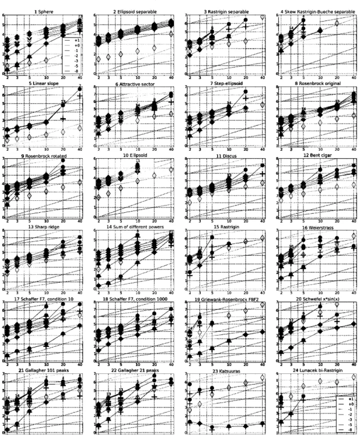
Fig. 1 . PSO expected r u n n i n g t i m e (ERT, <) t o r e a c h /o p t + A / a n d median n u m b e r off-evaluations f r o m successful triáis (+), for A / = 10Í + 1'°'_ 1'_ 2'_ 3'_ 5'_ S } (the exponent is given i n the legend o f / ] a n d /2 4) versus dimensión in l o g - l o g presentation. For each function and dimensión, ERT(Af) equals t o #FEs( Af) divided by the number of successful triáis,
w h e r e a t r i a l is successful if/o p t + A / w a s surpassed. The #FEs( Af) are t h e total n u m b e r (sum) off-evaluations w h i l e /o pt + A / w a s not surpassed i n the t r i a l , f r o m all (successful and unsuccessful) triáis, a n d /o p t is the o p t i m a l function valué. Crosses ( x ) indícate the t o t a l number of/-evaluations, #FEs(-co), divided by the number o f triáis. Numbers
above ERT-symbols indícate t h e n u m b e r o f successful triáis. V-axis annotations are decimal logarithms. The t h i c k light line w i t h diamonds shows the single best results f r o m BBOB-2009 for A / = l O- 8. A d d i t i o n a l grid lines show linear and quadratic scaling.
3.1. Differentiaí evoíution and PSO
Differential evoíution is, like PSO, a stochastic and population-based optimization technique. It was first introduced in 1996 by
Storn and Price [17]. Differential evoíution is capable of handling non-differentiable, nonlinear and multimodal objective functions and is fairly fast in doing so. DE has participated in the First
and was proven to be one of the fastest evolutionary algo-rithms.
The DE algorithm also works with a population of potential Solu-tions. The principie is same as PSO: a particle can gain by using information from other particles as well as the results of their own search. However, in the case of differential evolution, that information is sampled randomly. DE-PSO is basically a differential evolution algorithm mixed with ideas of particle swarm optimiza-tion[18].
PSO and DE define the population in the same way. It is
neces-sary to implement population and velocities as two 2-D arrays of data. The higher the dimensión, the more valúes each particle has. In order to initialize the velocities, one can either choose random valúes between the predefined bounds, or zero.
First, 3 random particles (ri, TJ, r-j) should be chosen in such a way that they are different from each other. The second task is to créate a mutated valué for each dimensión j of the particle according to the differential evolutionary algorithm.
When the mutation is done for every dimensión, the mutated one is evaluated with the fitness function, and then compared it to the evaluation of the non-mutated one, i.e. the current particle. If it is smaller, then the mutated particle replaces the oíd one in the population; in other case the particle swarm optimizer is triggered. If the DE-part of the algorithm does not find a better solution, PSO is activated. A new particle is created according to PSO formulas: velocity and new position. A basic velocity and position clamping is performed as well. We then just check whether the new valúes (velocity, position) exceeds the threshold defined in the algorithm. If the newly created particle is proven to be better, it is replaced by the oíd one for the next generation. Both personal best and global best particle vectors are updated as well. This whole process occurs over again until the Halt condition is reached.
More hybrid versions between particle swarm optimization and differential evolution have been proposed, for example the one proposed byjosé García, Enrique Alba andjavier Apolloni in:
"Noise-less Functions Black-Box Optimization: Evaluation ofa Hybrid Particle Swarm with Differential Operators" [19]. Their model is also simple
and is proven to obtain an accurate level of coverage range. The algorithm also contains 2 main parts. The first one is the differen-tial variation, in which new velocities and positions are calculated according to the following formulas:
Vy(t + 1 ) = W * Vy(t) + [1+0* (gbeStj ~ Xy)
xij(t + 1)=xij(t) + vij(t + 1)
j is the dimensión and í = l, 2, . . . population size, JJL is a scaling
factor (¡i = UN(0, 1)): and cp is the social coefficient (cp = LfN(0, 1)).
The second part is the mutation, which is calculated according to formula of DE. It is basically a new particle position between the specified bounds.
Figs. 1 and 2 show the benchmark results of both approaches
{PSO and DE-PSO) using the BBOB20W (Black Box Optimization Benchmark) with 24 noisy-free functions described in the
bench-mark procedure.
4. Neural network training using DE-PSO
Given a neural network architecture, every weight is coded as a genotype. Then we train the network by running the particle swarm optimization algorithm. The fitness function can be computed using
1 UN(0,1) function provides information about the uniform distribution on the interval from min = 0 to mea = 1 and generates random deviates. The uniform distri-bution has density/(x) = l/(max-mm) for min < x < max. UN(0,1) will not genérate either of the extreme valúes unless max = min or mea-min is small compared to min.
the mean squared error of the net with the training data set. Some variations aim to get better fitness valúes with more generalization properties just by running validation and testing sets.
Equations used in the particle swarm optimization training pro-cess are below: C\ and Cj are two positive constants, R\ and Rj are two random numbers belonging to [0,1 ] and w is the inertia weight. These equations define how the genotype valúes change along iter-ations; in other words this equations show how neural network weights change.
vin(t + 1 ) = wvin(t) + c^(pin -xin(t))+ (1)
C2MPgn - Xin(t)) (1)
xin(t + \)=xin(t) + vin(t + \) (2)
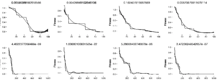
Previous equations modify the network weights until the Halt condition is reached, that is to say, either a lower mean squared error or a máximum number of iterations is reached. Figs. 3 and 4 show two examples of a neural network training using the DE-PSO algorithm, the XOR and the binary coding problems (Table 1).
Best neural network weights with a 8-3-3 architecture and com-puted by the particle swarm algorithm are shown in Tables 2 and 3 . These two neural examples reveal that the DE-PSO previously defined can be successfully applied to the training stage in order to solve the convergence of the algorithm when working with high dimensión individuáis. The XOR example with dimensión 9 and the binary-coding example with dimensión 39 are a good candidates to start with and to combine classical neural networks with swarm intelligence.
5. Grammatical swarm
Grammatical swarm (GS) [20] relates particle swarm algorithm to a grammatical evolution (GE); genotype-phenotype mapping to genérate programs in an arbitrary language [21]. The equations for the particle swarm algorithm are updated by adding new con-straints to velocity and location dimensión valúes, such tlS Vmax (bounded to ±255), and dimensión which is bounded to the range [0, 255] (denoted as cmjn and cmax, respectively). Note that this is a continuous swarm algorithm with real-valued particle vectors. The standard GE mapping function is adopted, with the real-values in the particle vectors being rounded up or down to the nearest inte-ger valué for the mapping process. In the current implementation of GS, fixed-length vectors are used, which implies that it is possible for a variable number of dimensions to be used during the program construction genotype-phenotype mapping process. A vector's ele-ments (valúes) may be used more than once if wrapping occurs, and it is also possible that not all dimensions are used during the map-ping process. (This can happen whenever a program is generated before reaching the end of the vector.) In this latter case, the extra dimensión valúes are simply ignored and are considered as introns that may be switched on in subsequent iterations.
5.1. Neural network topology using GS: first approach
Previous PSO model applied to a fixed neural network is a good training solution, however it does not define any kind or topol-ogy properties as it only obtains the best weight valúes. Following grammars can be used with grammatical swarm algorithms in order to obtain a network topology for a given problem.
This grammar can specify a feed-forward neural network topol-ogy with consecutive layers, that is to say, a classical multilayer perceptron.
<layers> :: = <layer> | <layer>, <layers> < l a y e r > : : = < d i g i t >
1 Sphere 2 Ellipsoid separable 3 Rastrigin separable 4 Skew Rastrigin-Bueche separable
2 3 i 10 20 40
5 Linear slope ?
-4
-4
5 .*•••*••' --"""H
l
f%~.
4 -4
>::: j .
'•"4
0 ^ = v . - - • ; • . ' . . ; . .; 1 ; . ..
2 3 5 10 20 6 Attractive sector
9 Rosenbrock r o t a t e d 1
i
r/^^r-^>
4
15—-<¡
^
r2 1 0
§ <
2 1 0_, ;
2 10
L*
- • • ' • ' •;".—-5 10 20 13 Sharp rídge
1 0 Ellipsoid
5
4
i Si
> : : *
2
1
0
A • Y
^
;;;;:,;2 1 0 V ~=ZZZ. 2 1
0 *¿í" • ' - '
2 J ¡ i 0 2 0 40
14 Sum of different powers
2 3 5 10 20 40 I S Schaffer F7, condition 1 0 0 0
7 7
r-r.
'."'
;:„"ZIÍ » <i /j
b^ f e 3
í
4
^
1 ^ H
K 2
^
r"
• ^r ' ^1
¿"
_._.
--.
1
i rt„_-¿ r'X £
2 } > i 0 2 0 4 0
2 3 5 10 20
7 Step-ellipsoid 8 Rosenbrock original
; , I..! A:-:rj „.-¿
Er:rr^4
5
-pdpxSfe
: *
;_:;;t
: *
, j -•""', |.;
TI'*
12 Bent clgar
7
2 J 5 10 20 40 15 Rastrigin
7 «.-*--
:;ÉIZ1.
5 4=
1 fKZA
5 4=
1 fJ
5 4=
1 fK*
5 4=
1 fP
r1í
--^"
r"
5 4
=
1 ff.
5 4=
1f _ . , t f
^ ' L j™
3 5 10 20 4 0 19 Griewank-Rosenbrock F8F2
*
'-" 1
s ^
' i
4 ¡P--A A-
._====£
5 V./ 3 S "i !^
^ _ = ^
; j p r " -
_----"
22 Gallagher 21 pe;
3 5 10 20 40 23 Kateuuras
SI
2 3 5 10 20 , 20 Schwefel x«sin(x)
<L^é^:z2*:ií
!
;
o .i^s=i-::4—i--.--,..-i
2 3 5 10 20 40 2 4 Lunacek bi-Rastrigin
B
7
: :«_ o _ i _
0.
i
3 -j"»
¿teg
&- - _-^>r
-i
3 -j"»
¿teg
-
• i . + 0 -1 -2l T
n r '
.±#F- ¡
:'J
-5 -8Fig. 2. DE-PSO expected running time (ERT, <) to reach/opt + A/and median number of/-evaluations from successful triáis (+), for A/= 10Í+1'°'_1'_2'_3'_5'_S} (the exponent is given in the legend of/i and/24) versus dimensión in log-log presentation. Foreach function and dimensión, ERT(Af) equals to #FEs(A/) divided by the numberof successful
triáis, where a trial is successful if/opt + A/was surpassed. The #FEs(Af) are the total number (sum) of/-evaluations while /opt + A/was not surpassed in the trial, from all
(successful and unsuccessful) triáis, and/opt isthe optimal function valué. Crosses (x) indícate the total number of/-evaluations,#FEs(-co), divided bythe numberof triáis.
Table 1
Binary coding: neural network pattern set and best fltness valué reached.
Input Output
Best fltness valué: 5 . 0 6 7 e - 0 5 .
0.0059O388182618566 0.00409949102646106 0.160407816687669 0.00670879911678114
4.4022377268488e-09 1.03680100831SOSe-22
20D 40D 6ÜD OÜD IODO
5.280084027408786-06 2.47236248542657e-07
8 0 0 IODO 2 0 0 400 600 000 1000
Fig. 3. XOR multilayer perceptron with 2 hidden neurons and a particle swarm optimization learning with 10 individuáis (individuáis have 9 dimensions). Each column
represents a different random initialization and each row a numberof iterations (100 and 1000).
0.448928449507574 0.380432955845818 0.166155810190459 0.0857910229358835
0.254269716684872
200
0.0718653921693906
100 150 200 250 300 300
0.0865752460809145 0.000314184787007479
Fig. 4. Binary coding neural network form 8 inputs to 3 outputs. First row is a neural network with 3 hidden neurons and second row a neural network with 5 hidden neurons.
Table 2
Binary coding: neural networkweights, fromthe input layertothe hidden layer, taking into account the bias term.
weight i, hidden neuron 1 hidden neuron 2 hidden neuron 3
input neuron 1 input neuron 2 input neuron 3 input neuron 4 input neuron 5 input neuron 6 input neuron 7 input neuron 8 Bias
0.1156528 -0.3683220 1.5325933 0.4830886 -1.5133460 -1.7465932 1.0519552 0.3397246 0.7092471
1.097272 25.945492 -9.765752 26.536611 0.790667 -3.369892 -4.920479 -1.924014 -5.304714
-0.946379977 -1.703378035 -0.636187430 0.002121948 -0.131921926 0.987214704 0.005404300 3.273439670 -0.331283300
Table 3
Binary coding: neural network weights, from the hidden layer to the output layer with the bias term.
weight i, output neuron 1 output neuron 2 output neuron 3
hidden neuron 1 hidden neuron 2 hidden neuron 3 Bias
1.261584 148.541038 -162.388447 0.090192
-4.759320 -1.054461 -2.017318 1.207254
0.9853185 -3.1161444 -3.4691962 1.9260548
Next grammar is able to genérate feed-forward connections not only with one consecutive layer but also with more than one con-secutive layer. Such connections are defined by the <connections> non-terminal, where the < d i g i t > means the n-consecutive layer.
< l a y e r s > : : = < l a y e r > | < l a y e r > , < l a y e r s > < l a y e r > : : = < d i g i t > < c o n n e c t i o n s >
-< c o n n e c t i o n s > : = -< d i g i t > | -< d i g i t >, -< c o n n e c t i o n s > < d i g i t > : : = 1 | 2 | 3 | 4 | 5 | 6 | 7 | 8 | 9
The whole algorithm is summarized as follows:
1 Créate an initial population of genotypes. 2 For genotype i
(a) Using genotype and grammar to obtain a neural architecture. (b) Compute fitness of genotype.
• Apply previous PSO algorithm to train the genotype net-work.
(c) Modified the best individual if appropriate. 3 Update velocity of genotype i.
4 Update position of genotype i.
5 If stop condition is not satisfied go to step 2.
This neural network model is a powerful one since only with the input and output pattern sets a network topology is chosen and also trained. Both tools, topology and training, are based on grammatical swarm and particle swarm optimization respectively, see Fig. 5.
Another useful approach could be to define a grammar with the weight valúes of neural networks connections instead of training the topology using a PSO algorithm.
6. Related work and experimental results
This work is focused in the development of methods for the evo-lutionary design of artificial neural networks. This paper focuses in optimizing the topology and structure of connectivity for these networks.
Artificial neural networks are well-established tools used with success in many problems such as pattern recognition, classifi-cation problems and optimization. The use of genetic algorithms in the evolution of neural networks has been widely used in the literature. However, in most cases limited experimental results are presented. In evolving a neural network using a genetic
algorithm, two main approaches are used. In the first approach, the network topology and the network weights are evolved simulta-neously [6,22-24], while in the second approach only the network topology is evolved and the parameters are estimated using a standard approach such as a gradient based optimization method [13,14]. Other approaches of defining the network's topology other than using genetic algorithms include pruning algorithms [13,14], simulated annealing based algorithms [13,14] and particle swarm optimization techniques [25-27,18].
The representation of the neural network is another important aspect of the evolutionary approach. Three major approaches are adopted in the bibliography. In the first, a binary coding of the topology and weights is used. In the second approach, a table struc-ture is used to represent the connectivity between the neurons and the network's weights. The third approach is considered the most sophisticated since it involves using a higher-level language such as a grammar to describe the network topology. The latter approach gives better control to the network architect since he can use créate node layers and better describe complex topolo-gies.
Evolutionary neural networks have been widely used in solv-ing various problems. Proposed method is tested against neural networks that are trained with various algorithms:
• RPROP [23] which is an improved versión of the well-known back propagation method local optimization method.
• A Powell's variant of the well-known BFGS [28] local optimization method.
• A global optimization method namely MinFinder [29] which is capable under some conditions, to find all the local mínimums of a function.
• Using and a genetic algorithm to estímate the neural net-work's initial parameters and the BFGS [30,31 ] local optimization method for fine tuning using a local search. This method is similar with the one described in [24]. In all cases, the function to be min-imized in the case of neural networks is the train error. In almost all cases, the proposed method outperforms its competitors.
-..
• -,
,
^ N s
'-X & V
^_ s
\ vil ' • S • 1
«. • i
**,
i> V-V '-N \ *• M v-} 1
* s
. , n -, . - . 1 "
— —
Fig. 5. Neural network topologies and training results obtained with a grammatical swarm for the topology and particle swarm optimization to train the net - XOR probiem - y axis: mean squared error vs. x axis: iterations.
6.1. Cíassification dataseis
• Wine: The wine recognition dataset (WINE) contains data from wine chemical analysis. It contains 178 examples of 13 attributes each that are classified into three classes.
• Glass: This dataset (GLASS) contains glass component analysis for glass pieces that belong to 6 classes. The dataset contains 214 examples with 10 attributes each.
• Pima Indians Diabetes: The PIMA dataset contains 768 examples of 8 attributes each that are classified into two categories: healthy and diabetic.
• Wisconsin Diagnostic Breast Cáncer: The Wisconsin Diagnostic Breast Cáncer dataset (WDBC) contains data for breast tumours. It contains 569 training examples of 30 attributes each that are classified into two categories.
• Circular Artificial data: The circular artificial dataset (CIRCULAR) contains 1000 examples that belong to two categories. The data in the first class belong to a circle and the data of the second class belong to a circular disc outside the first circle. Each example vec-tor has two attributes. It is expanded by adding 3 more attributes generated randomly (noise) using a normal distribution. • Spiral Artificial data: The spiral artificial dataset (SPIRAL)
con-tains 1000 examples that belong to two classes (500 examples each). The data in the first class are created using the following formula: x = 0.5 tcos(0.08t),y = 0.5rcos(0.08 + 7T/2), and the second-class data using: x = 0.5rcos(0.08r + 7r), y = 0.5rcos(0.08r + 37r/2), The original features vector has two attributes (x, y).
• Spiral Artificial data 2: The second spiral dataset (SPIRAL2) is cre-ated as the first dataset. Its difference is that its primitive set is expanded by adding 3 more noisy attributes using normal distri-bution.
• Liverdisorder: This dataset contains blood analysis data from peo-pie with liver disorders. It consists of 345 examples of 6 attributes each.
• Ionosphere dataset: The ionosphere dataset contains data from thejohns Hopkins Ionosphere datábase. It contains 351 examples of 34 attributes each that are split into two classes.
6.2. Regression dataseis
• BL: This dataset can be downloaded from StatLib (http://stat.cmu.
edu/datasets/). It contains data from an experiment on the affects of machine adjustments on the time to count bolts.
FA: The FA dataset contains percentage of body fat, age, weight, height, and ten body circumference measurements. The goal is to fit body fat to the other measurements.
LW: This dataset is produced from a study that was to identify risk factors associated with giving birth to a low birth weight baby (weighing less than 2500 g). Data were collected on 189 women, 59 of which had low birth weight babies and 130 of which had normal birth weight babies.
NT: This dataset contains data from a paper in the Journal of the American Medical Association that examined whether the true mean body temperature is 98.6°F.
PO: This dataset is available from StatLib (http://stat. cmu.edu/datasets/). It contains pollution data.
PW: This dataset contains numeric prediction data using instance-based learning with encoding length selection.
SN: This dataset contains data on a viticultural experiment that was conducted to investígate different methods of trellising and pruning.
MB: This dataset is available from Smoothing Methods in Statis-tics (http://stat.cmu.edu/datasets/).
BK: This dataset comes from Smoothing Methods in Statistics (http://stat.cmu.edu/datasets/).
6.3. Results
Results from the application of the proposed method against the methods RPROP, BFGS and MinFinder are Usted, see Tables 4 and 5 . Each method was tested for different topologies of the resulting neural network (e.g. the number of hidden neurons) and the topol-ogy with the best results was selected. The genetic algorithm's parameters have been estimated experimentally after observing that the algorithm converges faster using these parameters. The parameters are: máximum number ofgenerations: 500, population size: 500, chromosome length: 100, crossover rate: 0.95, mutation rate: 0.05, tournament size: 10.
Table 4
Test error for the classifications problems. All mentioned methods are compared against the proposed method, combination of grammatical swarm and particle swarm optimization (GS + PSO).
WINE GLASS PIMA WDBC CIRCULAR SPIRAL SPIRAL2 LIVER IONSPHERE
RPROP 0.5993 0.7137 0.3319 0.3271 0.4494 0.4906 0.5022 0.4356 0.1578
BFGS 0.4886 0.5393 0.3656 0.2091 0.0795 0.4531 0.4847 0.3886 0.1708
MINFINDER 0.1178 0.4941 0.3004 0.0489 0.0857 0.4343 0.4704 0.3559 0.1627
GENETIC 0.1426 0.4801 0.3216 0.0687 0.0784 0.4358 0.4815 0.3584 0.1699
GS + PSO 0.0541 0.5145 0.2133 0.0512 0.0811 0.4490 0.4880 0.3118 0.0999
Bold valúes represent the best obtained mean squared error.
Table 5
Mean squared error for the regression problems. All mentioned methods are compared against the proposed method, combination of grammatical swarm and particle swarm optimization (GS + PSO).
PO BL FA LW PW NT
Bold valúes represe nt the best obtained mean squared error.
SN MB BK
RPROP 0.34 0.57 0.94 0.51 0.17 0.56 1.08 0.49 0.54
BFGS 0.25 0.33 0.44 0.91 0.21 3.14 2.31 0.68 4.44
MINFINDER 0.26 0.21 0.25 2.41 0.27 1.72 1.13 57.94 3.06
GENETIC 0.29 0.26 0.29 2.01 0.22 2.81 2.04 8.45 13.64
GS + PSO 0.21 0.08 0.12 0.11 0.10 0.05 0.46 0.28 0.09
The experimental results show that the proposed method outper-forms the other methods, see Tables 4 and 5. Two major advantages of proposed model is that it is significantly faster than MinFinder by several orders of magnitude and is natively parallel. This gives it an edge over traditional methods since it can take advantage of distributed computing technologies.
References
7. Conclusión
This paper analyses a few optimization strategies in the natu-ral computation área. Some competitive and collaborative models have been described in order to understand the ability to extract some biological ideas and then apply them in computational mod-els. Such biological inspired models have proven to be a powerful tool in order to solve non-common problems in a collabora-tive/competitive way.
As a powerful application, neural networks can take advantage of such swarm optimization models. This paper has proposed a grammatical definition that chooses the best network topology by using grammatical swarm and network training.
Particle swarm optimization often fails when searching the global optimal solution when the objective function has a large number of dimensions. The reason of this phenomenon is not just existence of the local optimal solutions but also the degenera-tive process of the particles velocities (this means that particles stay in a subregion within the search área) [27]. This is a sub-plane which is defined by a finite number of particle velocities. Local óptima problem in PSO is object of study. New proposals are based on specific equations [26,25] which modify the basic particle. They use a randomized method (e.g. mutation in evolu-tionary computations) for either to maintain particles velocities or to accelerate them. Although such improvements work well and have ability to avoid falls in the local óptima, the prob-lem of early convergence by the degeneracy of some dimensions still exists, even when local óptima do not exist. Henee the PSO algorithm does not always work well for the high-dimensional function.
Usually, neural network parameters are in a high-dimensional space and then PSO algorithms are not very efficient ones when dealing with such individuáis. Best solution could be the integra-tion of PSO and GA in a new model GPSO taking advantages of both models, or at least to improve the impact of the high dimensional individuáis in the PSO algorithm.
[1] N. Agarwal, X. Xu, Social computational systems, Journal of Computational Science 2 (2011) 189-192.
[2] E. Bonabeau, M. Dorigo, G. Theraulaz, Swarm Intelligence: Form Natural to Artificial Systems, Oxford University Press, 1999.
[3] J. Kennedy, R. Eberhart, Y. Shi, Swarm Intelligence, Morgan Kauff-man, 2001. [4] T.Jayabarathi, S. Chalasani, Z.Z. Shaik, N.D. Kodali, Hybrid differential evolution
and particle swarm optimization based solutions to short term hydro thermal scheduling, WSEAS Transactions on Power Systems 11 (2007) 245-254. [5] N. Beji, B. Jarboui, M. Eddaly, H. Chabchoub, A hybrid particle swarm
optimization algorithm forthe redundaney allocation problem, Journal of Com-putational Science 1 (2010) 159-167.
[6] P. Haiguo, W. Zhixin, Z. Huaqiang, Cooperative-pso-based pid neural net-work integral control strategy and simulation research with asynchronous motor controller design, WSEAS Transactions on Circuits and Systems 8 (2009) 136-141.
[7] L. Ren, X. Jiang, G. Sheng, B. Wu, A new study in maintenance fortransmission lines, WSEAS Transactions on Circuits and Systems 7 (2008) 35-37.
[8] M. O'Neill, C. Ryan, Grammatical evolution, IEEE Transactions on Evolutionary Computation 5 (2001) 349-358.
[9] M.O'Neill,C. Ryan, M. Keijzer, M.Cattolico,Crossoveringrammaticalevolution, Genetic Programming and Evolvable Machines 4 (2003) 67-93.
[10] J.R. Koza, D. Andre, F.H. Bennett, M. Keane, Genetic Programming 3: Darwinian Intention and Problem Solving, Morgan Kauff-man, 1999.
[ 11 [ J.R. Koza, M. Keane, M.J. Streeter, W. Mydlowec,J. Yu, G. Lanza, Genetic Program-ming IV: Routine Human-competitive Machine Intelligence, Kluwer Academic Publishers, 2003.
[12] A. Neme, S. Hernández, O. Neme, An electoral preferences model based on self-organizing maps, Journal of Computational Science 2 (4) (2011) 345-352. [13] Y.H. Hu,J. Hwang, Handbookof Neural Network Signal Processing VE Profiling,
CRC Press, 2001.
[14] S. Katagiri, Handbook of Neural Networks for Speech Recognition, Artech House, 2000.
[15] P.M.A. Sloot,The cross-disciplinary roadtotrue computational science,Journal of Computational Science 1 (2010) 131.
116] J. Kennedy, R. Eberhart, Particle swarm optimization, in: Proceedings IEEE Inter-national Conference on Neural Networks, volume IV, 1995, pp. 1942-1948. [17] R. Storn, K. Price, Minimizing the real functions of the icec'96 contest by
differ-ential evolution, in: IEEE Conference on Evolutionary Computation, 1996, pp. 842-844.
[18[ M. Pant, R. Thangara, C. Grasan, A. Abraham, Hybrid differential evolution—particle swarm optimization algorithm for solving global opti-mization problems, in: IEEE International Conference on Digital Information Management, 2008, pp. 18-24.
[19] J. Garcia-Nieto, E. Alba,J. Apolloni, Noiseless functions black-box optimization: evaluation of a hybrid particle swarm with differential operators, in: Genetic and Evolutionary Computation Conference, 2009, pp. 2231-2238.
[21] M. O'Neill, A. Brabazon, Grammatical swarm, in: Proceedings of the Genetic and Evolutionary Computation Conference, 2004, pp. 163-174.
[22] G.G. Yen, H. Lu, Hierarchical genetic algorithm for near-optimal feedforward neural network design, International Journal Neural Systems (2002) 31-43. [23] M. Riedmiller, H. Braun, A direct adaptive method for faster backpropagation
learning: the rprop algorithm, in: Proceedings IEEE International Conference on Neural Networks, 1993, pp. 586-591.
[24[ V.M. Rivas, JJ. Melero, P.A. Castillo, M.G. Arenas, J.G. Castellano, Evolving rbf neural networks for time-series forecasting with evrbf, Information Sciences 165 (2004) 207-220.
[25] T. Hendtlass, A particle swarm algorithm for high dimensional, multi-optima problem spaces, in: Proceedings of Swarm Intelligence Symposium, 2005, pp. 149-154.
[26] K. Parsopoulos, V.P. Plagianakos, G.D. Magoulas, Stretching technique for obtaining global minimizers through particle swarm optimization, in: Proceed-ings of Particle Swarm Optimization Workshop, 2001, pp. 22-29.
[27] M.R. Rapaic, Z. Kanovic, Z.D. Jelicic, Atheoretical and empirical analysis of con-vergence related particle swarm optimization, WSEAS Transactions on Systems and Control 11 (2009) 541-550.
[28] M.J.D. Powell, A tolerant algorithm for linearly constrained optimization calcu-lations, Mathematical Programming 45 (1989) 547-566.
[29] I.G. Tsoulos, I.E. Lagaris, Minflnder: locating all the local minima of a function, Computer Physics Communications 174(2006) 166-179.
[30] C.G. Broyden, The convergence of a class of double-rank minimization algo-rithms, Journal of the Institute of Mathematics and Its Applications 6 (1970) 76-90.