Application of global numerical procedures to the analysis of shells

APPLICATION OF GLOBAL NUMERICAL PROCEDURES

TO THE ANALYSIS OF SHELLS

Avelino SAMARTIN

Universidad Politecnica de Madrid

Department of Structural Mechanics

E. T.S./ de Caminos, Canales y Puertos 280.40 Madrid, Spain

E-mail: samartint!)cami nos. u pm .es

Abstract

Examples of global solutions of the shell equations are presented, such as the ones based on the well known Levy series expansion. Also discussed are some natural exten-sions of the Levy method as well as the inherent limitations of these methods concerning the shell model assumptions, boundary conditions and geometric regularity. Finally, some open additional design questions are noted mainly related to the simultaneous use in analysis of these global techniques and the local methods (like the finite elements) to finding the optimal shell shape, and to determining the reinforcement layout.

1.

Introduction

The shallow curved plate theory of linear elastic thin shells is assumed. Details can

be seen in [1). A right hand cartesian axis (x1,X2,z) is used to describe the middle shell

surface by means the following parametric equations:

The following notation is used:

• Indexes i and j vary between 1 and 2

(i ::/:

j).

• 6;i is the Kronecker delta.

• Einstein summation convention applies unless the contrary is explicitly stated.

• Comma notation with index i is used to represent partial derivatives respect to a;.

• X;, Z are the pressure force components on the middle surface.

• u;, w are the displacement components at a point of the middle surface.

• n;₁ and q; are the force stress-resultants of the stresses Uij and Uiz.

• m;1 are the couple stress-resultants of the stresses U;j.

• A;i arc the coefficients of the first fundamental form of the middle surface. It is &'iSnmed A;1

= 0.

• 1\;j are the curvatures of the middle surface.

• h is the constant shell thickness, E the Youngs modulus, v the Poisson ratio,

Eh 3 Eh

D

=

₁₂(1~v2) and K = ~·

The equilibrium equations of a differential shell element are:

n;j,j +X; 0

ffiij,j -q; 0

K;inii

+

q;,i

+

Z 0

• Strains/ displacements

1

e · · _IJ

= -

₂ (u · · _I,J

+

u · -_J,l 2K _IJ w)

k;j = -W,ij

• Stress-resultants/strains

• Strcss-rcsultants/ displacements

n;;

=

K(u;,;

+

vu_{1,1 -} (K;;

+

vK₃j)w)

n;3 = K[u;,i

+

Uj,i - 2K;iwJ

r; = q;

+

m;i,j = -D(w,;;;

+

(2-v)w,jjj)

in which r; are the Kirchhoff shears and '\72 =

f;.r

+

f;.r.

I 2

The governing differential equations expressed in terms of the normal displacement

w and the Piicher stress function <I>, defined by the expression (not summed) n;i = (-)'+J<f>,₁ - l i ; j

J

X;da;, are:

D'\74w- V'k<I>

=

Z- K;;

f

X;da;

'\74<1>- Eh'\72Kw

=

jx ·

I,JJ do·+ l vX · 111

• · 2

e

2

e

2

m whtch '\7 K = J<;; ~-K;i ~·

j ' 3

In the case of '\7~ =f-'\72 the Ambartsuyam function W is normally introduced [3) to

obtain the complementary solution by solving a single differential equation:

vsw

12(1 - v2) '\74 lV = 0

+

h2 K

in which w = '\74lV;<I> = -EhVi-W.

In the other case (Ku = K22; K12

=

0 i.e. spherical shallow curved plate) the

Mishonov function is used instead, defined as: '\72w = '\72W;'\72<1> = -EhK'\7~ W, and

the same single differential equation as before is reached except the coefficient of second

term is now multiplied by K.

2. Description of the Levy solution.

Rectangular planform, curvature lines ( K12 = 0) and normal gable boundary

condi-tions along two opposite edges of the shell are assumed, i.e.:

n11 =O;u2=0;w=O;mt1 =Oalongo1 =O,Lt

For brevity only the case with different curvatures is shown. The spherical solution

The solution is expressed by sum of harmonic terms. For each term a vector R of dimension 15x1 containing the results of interest in the analysis is defined as follows:

in which each element is a function of 02 and varies along the direction 01 as sin >.o1

except the terms 1, 4, 8, 11, 12 and 14 which vary as cos >.o1, >.

=

n [

1 corresponds to

the n-th expansion term. The expression of this vector of results is given as sum of a particular and the complementary solutions (2]:

in which G is a 15 x 8 matrix shown in table 1. C;

=

(Ci, C~] is a partitioned matrix of dimension 8 x 4 and the k-th row of the 8 x 2 submatrix Cj is t;k (pr cosk~.p;, p~ sin k~.p;]

with €a

=

(-1)\~:2k = 1;k = 0,1, ... ,7,p; = (r~ +s~)! and r; and s; are constants

depending on the real and imaginary parts of the roots of the characteristic equation,:

.

_[a;+~]!·.- [-a;+~]!

r,- 2 ,s,- 2

2 ( i

I

-K?

+

6. [Kt+ 6. ( )' K2-Kl ]

a;=>.- -l)p.y 2 ;b;=p. 2

+ -

1 K 1 IK2-K1I

J3(1- v2) ).4

P. = h ; ~ = Kt+ 4(Kl - K2)2 p.₂

The square matrix P(x) = (Pt;(x)],x

= 02,/32

= £2- 02 of dimension 4

is

parti-tioned in 4 submatrices of dimension 2 X 2. Each of these submatrices has the following

expression:

P;;(x)

= [

Pi! (x)

-p;2(x) Pi2(x) ]

n ( ) 0 -r·z -r·z ·

( ) ; r;; x

= ;

P••

=

e ' coss;x; P12

=

e ' sms;x

Pi! X

The eight arbitrary constants A;i, B;; are contained in the two 4 X 1 column matrices

These constants can be found by imposing the arbitrary boundary conditions along the edges o2 = 0, L2

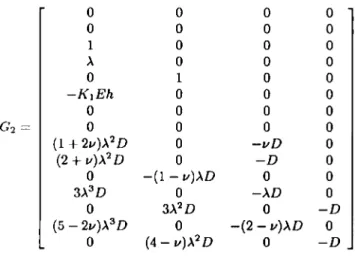
TABLE 1. Matrix G = [G1,G2]

( -I<1

+

vl<2)>.3 0 -K2>.

+

{2

+

v)K1>. 0

0 K1>.2- {2

+

v)K2>.2 0 K2 +vK1

>.4 0 -2>.2 0

>.5 0 -2>.3 0

0 >.4 0 -2>.2

0 0 Ki>.2 Eh 0

-K2>.4Eh 0 K1>.Eh 0

G1= 0 -K2>.3 Eh 0 K1>.Eh

>.6 _{0 -{2}

₊

_v)>.4 _{D 0}

v>.6D 0 -(1

+

2v)>.4 D 0

0 -(1

+

v)>.5 _D

0 2{1- v)>.3 D

>.' D 0 -3>.5D 0

0 >.6D 0 -3>.4D

). T lJ _{0 -(4- v)>.}5 _{D 0}

0 0 0 0

0 0 0 0

1 0 0 0

>. 0 0 0

0 1 0 0

-K1Eh 0 0 0

0 0 0 0

G2 = 0 0 0 0

(1+2v)>. 2D 0 -vD 0

(2 + v)>.2 D 0 -D 0

0 -(1-v)>.D 0 0

3>.3D 0 ->.D 0

0 3>.2D 0 -D

(5- 2v)>.3 D 0 -(2-v)>.D 0

0 (4- v)>.2 D 0 -D

3. Extensions of the Levy process.

The Levy formulation just described can be extended [2) to treat quite general systems of shallow shell structures, with transversally variable thickness or curvature changes, by introducing the standard methods of matrix analysis of structures, such as the stiffness method, along the transversal shell direction, i.e. the 02 direction. By a suitable selection

of columns and rows of the matrix G and the vector

Ro

the two following relations can

be reached:

[

~~

] =

~

+

Gd [

~

] ; [

~

]

=

po

+

Gp [

~

]

in which p; and d; are the vectors of the forces and displacements along the border

02 = 0 and 02 = L2 respectively, i.e., the vectors with components n12,n22,rl,m22

and u1, u2, w, W,2· By elimination of the constants A and B the stiffness fundamental

equation is obtained:

[

~

] =

Po - kdo

+

k [

:~

]

with k = GpG~ 1 the 8 X 8 stiffness matrix.

To treat other boundary conditions than the normal gables in the two opposite edges

01 = 0, L1 several attempts have been made. The first introduce further approximations

in the theory [4], in such a way that the derivatives of order 6 and 2 in the direction 01 disappear. Some typical approximations are summarized in table 2. In these cases the trigonometric functions sin >.o1 and cos>.a1 used in the Levy process can be replaced by

the new orthogonal set of functions in

[0,

L1 ), known as Raleigh functions, 4>(at). These

functions satisfy more general boundary conditions than the normal gable ones along the two opposite shell edges and they are defined by the eigenvalue problem: 4>,tlll +.>.44>

=

0 and the general homogenous boundary conditions. In the formulation of the equations of table 2. the static-kinematic analogy of Goldenweizer (5] has been considered.

Table 2. Approximations of the shell equations.

Approxi1nations General Plate Shallow Curved Plate

State Functions Name Urder derivatives Name Urder derivatives

owp;;l<'<'l<>d

"'•

__l "'2

_"'•

_l "'2

I !\'one - 8,6,4,2 8,6,4,2 _Jenkins Don ell 8,6,4,2 8,6,4,2

2 1U.t2. ~12 - 8,4 8,6,4,2

-

8,4 8,4

3 fUt2• t':t2 Vlasov 4 8,6,4 Schorer 4 8

1lltl' l22 tvb

particular solution and may be a double trigonometric series i.g. the Navier solution.

The complementary solution is constructed of two groups of linear independent Levy

solutions, along of each the directions a1 and 02. The procedure combines suitable

sets of Levy solutions with the particular solution to satisfy all the boundary conditions

simultaneously. Good convergence has been reported mainly for kinematic boundary conditions.

Finally Michael [7] has developed several strategies to extend the Levy process to

more general boundary conditions. The line techniques has been applied to the direct differential equations either in the two variables (normal displacement and stress func-tion) or in the three displacements. Indirect solutions i.e. those using a variational

approach or a

n ..

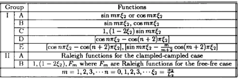
,leigh-Ritz method with or without Lagrange multipliers have proven to

be efficient even with "difficult" boundary conditions. In table 3 the functions selected in these methods arc shown. The suitable selection of these approximating functions is essential for the convergence of the methods.

Table 3.- Approximating functions

Group Functions

I A sin m7T{2 or cosm7T6

B sin m7T{2, cosm7T{2

c

1, (1- 26) sin m7T{2

D [cosn7T{2- eos(n

+

2)11"{2]

8 [cos n7T{2- cos(n

+

2)11"{2], [sin m7T{2- m~ cos(

m+

2)11"{2]

II A R.aleigh functions for the clampled-campled case

B 1, (1- 26), Fm where Fm are R.aleigh functions for the free-fre case

m=

1,2,3,···n=0,1,2,3,···6 =I!

The functions lA, IB, IC and liB have been used by Chuang and Veletsos, while

Noor and Veletsos have used IB and ID. The functions lA, IIA and liB are orthogonal

functions. The functions ID satisfy the clamped boundary conditions but produce zero normal and Kirchhoff shears on the boundary. They have been proposed in [8] when

they are referred as alnwst ortlwgonal functions. The functions lE have been obtained

by modifying ID to avoid the zero shears along the boundaries. However, the shape of the subgroups of lE arc similar, and numerical difficulties are foreseen if more terms

are considered. The functions IIA and liB have been used with the three displacements

formulation of the shell equations. Some essential or kinematic boundary conditions are not satisfied by some groups of these functions and in these cases Lagrange multipliers have been used.

4. Conclusions.

Shown abo\·e are several global numerical techniques that have been successively applied during the past for the analysis of shells. However, with the advent of the FEM and related numerical methods, global solutions had diminished use in shell analysis. Nevertheless, in the author's opinion, the simultaneous use of these solution techniques for the regular or smooth part of the shell structure and the application of a discretized model for the borders and the most irregular part of the shell can be a an efficient compromise.

Finally it is important to point out that shell analysis represents only a part of the

more comprehensive task of the shell design. Problems of optimal shell shape finding, reinforcement of concrete shells and construction procedures must also be considered.

1. V. Z. Vlasov Geneml Theory of Shells and its Applications to Engineering

NASA. 'ITF-99 (1964).

2. A. Q. Samartin and J. Munro Dynamic Analysis of Translational Shells CSTR

3. S. A. Ambartsumyan On the calculation of shallow shells NACA. TM-1425

{En-glish translation from Prikjanaya Matematika i Mekhankia, Vol 11 {1947).

4. J. Munro The Linear analysis of thin shallow shells Proc. Inst. Civil Engineers,

Vol 19. (1961).

5. A. L. Coldenweizer Theory of elastic thin shells Pergamon Press {1961).

6. D. A. Cuna...--ekera Numerica.l analysis of thin shells PhD Thesis University of

London (1967).

7. K. C. t-.1ichael and J. Munro Approximating functions and indirect solutions of

shell prvblems Proc. of the lASS Conference (Mexico, 1967)

8. M. M. Filoncnko-Boroditch On a system of functions and its applications in the