Modeling and numerical sensitivity study on the conjecture of a subglacial lake at Amundsenisen, Svalbard

Modeling and numerical sensitivity study on the conjecture

of a subglacial lake at Amundsenisen, Svalbard

D. Mansutti , E. Bucchignani , J. Otero , P. Glowacki

A B S T R A C T

We present a new numerical procedure to assess the plausibility of a subglacial lake in case of relative small/moderate extension and surging temperate icefield. In addition to the flat signal from Ground Penetrating Radar remote survey of the area, early indication of a likely subglacial lake, required icefield data are: top surface elevation and bathymetry, top surface velocity at some points, in-depth temperature and density profiles of upper layer. The pro-cedure is based on a mathematical model of the evolution of dynamics and thermo-dynam-ics of the icefield and of a subglacial lake. The Glen's law is adopted for ice rheology and Stokes reduction is applied; Large Eddy Simulation technique is used for the lake. Ice/water phase change is described. Finite volumes for model discretization and a front-tracking tech-nique to follow the moving interface characterize the numerical method.

We have applied this procedure to the case of a subglacial lake conjectured in the area of Amundsenisen, Svalbard, and, here, the results of a sensitivity study are discussed. In partic-ular we point out that the effect of firn and snow upper layers on the system, in terms of temperature field, density and water content, has to be included in the modeling, as it con-tributes to the overcoming of the ice metastable state and the release of subglacial water. Accordingly, ice water content changes have to be carefully described. The depth of the bed depression is confirmed to be critical for the formation of the lake.

1. Introduction

The fact that icy moons of the solar system, such as Europa and Enceladus, are known to have oceans of water beneath their thick ice crusts, has further increased the importance to study the polar subglacial hydrology, for the similarities between the two environments and the possible extended use of the gained knowledge [1,2]. The attention is, here, focused on polar subglacial lakes.

(mirror-like) surface with slopes less than 1%. Nevertheless a water film on a flat rocky bottom has very similar character-istics and might be interpreted erroneously as being a sub-glacial lake.

The principal aim of this work is to provide a new mathematical numerical tool for seeking additional hints on the plau-sibility of the existence of a subglacial lake based on the equations of the dynamics and thermo-dynamics of the grounded icefield and a conjectured subglacial lake.

Incorporating the appropriate ice constitutive law (Glen's law) (see Paterson [5]), we have extended to this application well-tested modeling and numerical simulation tools developed by two of the authors for solving moving boundary prob-lems in materials science (metal melting/solidification, artificial crystal growth) [6-8] and for the evolution of the icy crust of Europa [9].

We have considered the case of the Amundsenisen Plateau at Southern Spitzbergen (Svalbard archipelago), an icefield of about 80 km2 in area, where radio-echo sounding measurements show high intensity returns from a nearly flat basal reflec-tor at four zones, all of them with ice thickness larger than 500 m [10]. These reflections might correspond to subglacial lakes. In order to determine whether, in one of those zones, a subglacial lake is compatible with other measured quantities, such as density and temperature of ice upper layer and ice surface velocities, we propose to simulate the system at fixed measured conditions, lake included, by solving numerically the model introduced and, then, check the compatibility of the results.

This paper is organized as follows: in Section 2, the mathematical model is introduced; in Section 3, the finite volume solution procedure is sketched; in Section 4, the physical problem at Amundsenisen is described and the simulation plan for the conjecture check is proposed; in Section 5, the numerical results of sensitivity tests are presented and discussed and, in Section 6, conclusions are drawn.

2. Mathematical modeling

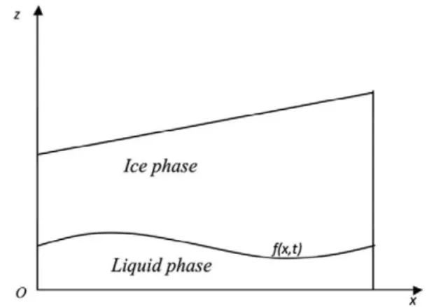
A prototypical space geometry, as in Fig. 1, is considered, that is a 2D section with an icefield, flowing from left to right on a rocky bottom, and a subglacial lake, that has been conjectured under the icefield in correspondence of a bed depression. Depending on external temperature history, the interface of ice with atmosphere might have very complex rheology in cor-respondence of the snow layer and the firn layer, the last one formed from water and ice sublayers resulting from successive refreezing events with compression.

The mathematical model adopted is based on the classical mechanics laws and principles: for the icefield, we refer the reader to Greve and Blatter [11] and, for phenomenological aspects of glacier physics, to Paterson [5]; in addition, references focussed on subglacial lakes and taken into account in this work, are Thoma et al. [12-14].

2.1. Icefield equations

Ice crystals have a structure that allows continuous deformation in response to an applied shear stress (creep, fluid-like behavior) in a way that is dependent on the direction of stress relative to the crystal planes (anisotropy). However ice con-sists of a huge amount of crystallites (polycrystalline ice) and the single crystal anisotropy averages out in the compound which exhibits an isotropic macroscopic behavior. Elastic deformation, primary, secondary and tertiary creep are the subse-quent deformation phases that a polycrystalline ice sample undergoes due to constant shear stress. Such a non-newtonian rheology is satisfactorily described by the Glen's law, a power law of the deformation gradient components for the effective viscosity of ice ¡i¡ [5,15], that is

Hi = 2-(1+n)/2M-1/"{fr(D2)}1~"/2" (1)

z

O

x

Fig. 1. Prototypical problem geometry.

tlrn

ice

being ü, the velocity vector, D = \\ VÜ + (Vü)T the rate of strain tensor, tr the trace operator, A the so called flow rate func-tion, and n a constant ranging between 1.5 and 4.2. The function A is an Arrhenius type function of the temperature I,

A=A0exp(-Q_/RT), (V)

with Q_= 60 -f-139 kj mol- 1 [5], the activation energy for creep, and R = 8.314 J mol_1K_1, the universal gas constant. The flow rate factor, A0, does not depend on temperature but it may depend on pressure or water content of ice or crystal size and

orientation according to the actual natural setup. For cold ice at temperature T > 263.15 K, the constant value for the flow rate factor amounts toA0 = 1.733 x 103 Pa~3 s. We observe that with exponent n unitary, p¡ reduces to Newtonian viscosity.

Restricted to the cases where the incompressibility constrain applies, the icefield equations for momentum and mass con-servation laws are written in the following form:

A f^ = - V p + V • {ft- [Vu + (Vu)du — — \ / n _ i _ \ / . ; / / i \ / T / _ i _ i \ / T M i *. _i_ n . c r T]} + Pig

(2) V ü = 0.

with pi} the density amounting to p¡ = 910 ^ , p, the pressure and g, the gravitational acceleration. The advective term is

neglected for the characteristic slowness of the ice motion.

The 2nd order PDEs system, (1), ( 1'), (2), results determined via the assignment of initial and boundary conditions that will be discussed later.

2.1.1. The case of temperate ice

In Arctic, and also in the mountains at non-extreme latitudes, ice might be temperate, that is a mixture of water and ice agglomerates at pressure melting point temperature, Tm (locally metastable state).

The Clausius-Clapeyron law for Tm represents one of the counterintuitive behaviors of the water molecule, as Tm

decreases with increasing value of pressure p:

Tm{p) = T0-Pp, with p = 9.7456 - l O ^ K P a- 1, (3)

being I0 = 273.15 K, the value of ice melting temperature at low pressure. Then, in the case of temperate icefields, the ther-mal field is known and we are allowed to neglect the equation for energy balance.

Furthermore, the flow rate function A in the Glen's law has to be specifically detailed.

According to Duval [16], who developed mechanical tests on ice samples of temperate glacier, the linear relation

A = (3.2 + 5.8W)10"2 4Pa-3s-1 (4)

with W, the water content of ice in per cent, fits the data up to tertiary creep and is valid for n = 3 and water content up to 1% (essentially in the case of water present in veins confined by three to four grains, due to pressure or strain heating melting). The average value W= 0.33 [%] is often used in the literature; actually, it holds at the basal ice layers, the most important in glacier flow, and is also adopted here.

Another expression of the flow rate function, A, and related water content correlation, W, have been proposed by Breuer et al. [17] using characteristic data typical of King George Island temperate ice cap (South Shetland Island, Ant-arctica). For the physical similarities of that icefield with the one considered in the present work, we report those func-tions below.

Starting from Lliboutry [18] theoretical argument on the increase of water content with depth due to strain heating and from Vallon et al. 's variation law of water content with depth [19], Breuer et al. fitted their data to a fourth-power depen-dence of water content with ice normalized thickness.

Called zmin(x) and zmax(x) respectively the value of the z coordinate a.s.l. (above sea level) of bottom and top icefield surface at the abscissa x, the estimate of the water content W as a function of zmax(x) and of the normalized thickness,

Zn = (Z- Zmin(x))/(Zm a x(x) - Z m i n M ) . r e s u l t s :

0.6 • exp (1 - z„)4, at zmax(x) < 400 m

W(z„,zmax) = ^ J 2¡ E? ^ M . o . 6 - e x p ( l - z „ )4, at 400 m < zmax(x) < 675 m (5) 0, at zmax(x) > 675 m.

For the sake of clarity, in the following function, temperature is measured in °C and transformed into T* = T + ¡5p, in order to overcome the dependency of the melting point on pressure; then, assigned:

(6)

A{T ,W) =

(1 + 1.81 -W), l"l 01 i f-\ w \

^l.Ul + ^l 0 6 e x p ( 1 )J

= [l + ( l + f ) - 1 . 8 1 2 5 • (0.925 + 0.084 - T ) , (0.855 + 0.07 - T ) ,

•0.126

W],

• r].

atT

at at at

--2 -5 -8

0°C

< c

sj

proposed flow rate function has the following expression:

A=A{T,W)-3M\ - l O - ^ P a ^ s -1. (7)

Let us notice that Duval's (4) and Breuer et al.'s (6) and (7) formulas meet at pressure melting temperature when W = 0.33 is assumed. The additional evaluations at lower ranges of temperature pertain to the firn and snow layers upon the temper-ate core of the glacier. The total thickness of the two superficial layers amounts typically to 25-30 m.

2.1.2. Boundary conditions

2.1.2.1. Atmosphere/icefield interface. In this work we limit the modeling to the treatment of steady ice upper surface. In this case non-null accumulation/ablation rate as implies non-null velocity of the accumulating/ablating phase (here, ice); fixed Fs(x, t) = s(x, t) - z = 0, the equation of the upper icefield surface, and called ns = ^^, its normal unitary vector, the boundary condition reads

-ü-ñs = as. (8)

The interface normal velocity (here, supposed to be zero) is in general different from the normal velocity of the interfacing phases. In the present case, when snow falls, it pushes down ice to the ground so that the external icefield surface keeps the same position though ice at the surface moves inward according to the determined velocity.

However, as data on as are fragmentary and insufficient, for steady upper surfaces, the following condition

T • ns = 0 (8')

is, here, preferred. This condition results from the atmosphere/icefield momentum jump condition where the contributions of the advective term and the atmospheric stress are neglected for being relatively smaller compared to the icefield stress. 2.1.2.2. Icefield/rocky bottom interface. With basal temperature at pressure melting point, the phenomenological Weertman-type sliding condition, quantifying the basal sliding velocity of ice, vb, might be adopted; fixed Fb(x, t) = b{x, t) - z = 0, the

equation of the lower icefield surface and called ñb = ^¡^; its normal unitary vector, the condition reads: IIVFbll

T P

u=vb = Cb^tb (9)

with T • ñb = xbtb +Nbñb, the stress undergone by the icefield at the rocky bottom (xb, basal shear stress, and Nb, normal

stress), p andq, integer exponents modulated according to the specific natural set-up ((p,q) = (3,1) or (3,2) for sliding on hard rock and (1,0) for sliding on soft, deformable bottom) and Cb, a constant to be tuned according to available data.

2.1.2.3. Left and right outlets. The prototypical geometry considered in this work is characterized by open right and left ver-tical boundaries, respectively a glacier outlet and an ice divide, this one being an ideal verver-tical plane where ice flows down-ward and departs away from it at both sides. Here, the ice velocity field undergoes homogeneous Neumann or Dirichlet condition as in the following:

^ = 0 (outflow) (10)

Bv

u = 0, 4f- = 0 (vertical flow). (11)

The condition (10) holds far enough from the ice divide. The condition (11) enforces the symmetry of the vertical com-ponent of velocity with respect to the ice divide (that is maximum/minimum point locus of v).

2.2. Subglacial lake equations

In describing the hydrodynamics of a subglacial lake it is necessary to take into account the occurrence of turbulence phe-nomena that we have chosen to face by the Large Eddy Simulation (LES) approach [20]. In this modeling context, in the liter-ature on the Antarctic subglacial lakes, Thoma et al. [12], point out the typical dominance of the background viscosity on the velocity so that the use of constant eddy viscosity and diffusion coefficients appear to be preferred to the Smagorinsky approach resulting in unnecessary complications. Then, the equations adopted for the subglacial basin hydrodynamics follow:

9 U , V7 XT', — 1 V7„ , V7 ÍAMY7,-I\ , P-A

dt Po ^ V J p0a' (12)

V 0 = 0.

(equation of state) is taken into account: the expression of the water density pw, as provided by Chen and Millero [21] in

1986, is adopted; with a precision better than 2 x l C T6g c n r3 within the validity ranges, [0-0.6] for salinity, [0-30 °C] for temperature and [0-180 bar] for pressure, it has the form:

pjp) = p0(l - p/fc) with p0(g cm-3) = 0.9998395 + 6.7914 x K T T - 9.0894 x l ( Tbr

+ 1.0171 x 1 0 "7r3- 1 . 2 8 4 6 x l 0 -9T4 +1.1592 x l 0 - " T5- 5 . 0 1 2 5 x lO"1 4!6 + (8.181 x l 0 ~4- 3 . 8 5 x 10-6T + 4.96x 10-87"2)S,

and k{bar) = 19652.17 + 148.113 • T - 2.293 • T2 + 1.256 • 10_2T3 - 4.18 x l o "5!4 + (3.2726 - 2.147 x 10_4T + 1.128 x 10~4r2)p + (53.238 - 0.313 • T + 5.728 x 10~3p)S

(13) where p0 and pw(p) are respectively the density values at sea level (p = 0) and at pressure value p, and S is the salinity.

For the choice of the LES coefficients AM = (A",A"\ also called Eddy Viscosity Coefficients (EVC), we have developed

numerical tests on the specific geophysical set-up of the experimental case that will be presented later; we have also taken into account the numerical results by Thoma et al. [12], on the Vostok and Concordia subglacial lakes in Antarctica. Cited authors obtain that the eddy viscosity coefficients can be estimated via this formula:

M LxU M M 6

Ah = ^ — , Av <xAh x 10 (14)

where L and Li represent the reference length of the lake geometry and the reference horizontal advection velocity. In par-ticular, for the Vostok lake, they have chosen A" = 50 m2/s leading to Li = 1 mm/s. We have adopted this value of the refer-ence velocity as target in the numerical tuning of LES coefficients; in fact a direct measurement of the true velocity is not possible.

The energy equation for the water subglacial basin has the form:

|+( f l . V ) T = V . ( # V T )+ ]¿ - *w (15)

where <DW, the dissipation term is assumed negligible. The thermal diffusivity vector-valued coefficient AH = (A",A"), whose

components are called Eddy Diffusion Coefficients (EDC), is evaluated in terms of AM and of the directional Prandtl numbers, AM AM

defined as: Prh = -4¡, Pr¡, = ^+. Thoma et al. [12], successfully experimented the following ranges for the Vostok lake: (a) Prh = Prv = 0.2 -=-10 and (b) Prh = 1 and Prv = 0.2 -=-10.

2.2.1. Boundary conditions

2.2.1.1. Subglacial water/rocky bottom interface. On the rocky bottom of the basin, no-slip condition would be ordinarily asso-ciated to the momentum equation:

u = 0. (16) However LES formulation does not describe the flow structures within the corresponding boundary layer but only their

dynamical impact through ad hoc choice of the value of the eddy viscosity and diffusivity coefficients, EVC and EDC. Then, in the vicinity of the solid boundary, only grid-sized flow structures, undergoing free-slip, are detected and the vector boundary condition (16) changes into the following scalar ones:

^ = 0

dn (16') u„ = 0,

with ut and un, the tangential and normal velocity components.

The geothermal heat flux qgeo is assigned in order to determine the solution of the thermo-dynamical model of the basin:

^^+^W=

^>, (17)

with cw, the subglacial water heat capacity, and ñb = (n6x,n6z), the normal unitary vector pointing inside the lake. In the literature, the value of qgeo is estimated within [35 mW/m2, 50 mW/m2].

In this paragraph superscripts w and i are added to the symbols of the unknowns in order to distinguish the phases; n = (nx,nz) stands for the unitary vector normal to the interface, pointing inside the icefield.

At the interface, here, considered, water, ice and the interface itself move at each own velocity.

Concerning boundary conditions to ice flow, the size of the subglacial lake has to be taken into account. When the ratio of the length of the lake over the average ice thickness is very large, ice behaves like in a ice shelf that is no shear stress applies at the interface; for example, above Vostok lake (50 km long), an increase of velocity towards the center of the lake (extension flow) followed by a decrease in ice speed passed the lake (compression flow) and a slight turning of the ice flow over the lake are revealed by the surface velocity field determined from radar interferometry (see Kwok et al. [22]). In Antarctica average ice thickness is R¿4.5 km. In that case, the boundary conditions to be imposed result the following:

ff = 0, 4 = 0 (18')

where u[, u\ are the tangential and normal component of ice velocity to the interface. When the two-dimensional reduction is applied, alike in the present case, Weertman-type sliding condition (9) is to be extended also to this portion of the bound-ary. On the other hand free shear stress condition would induce ice rotational motion that is not supported here. Then, two dimensional reduction of the modeling has the implication to neglect the action of the lake onto the icefield dynamics and is admissible only when the ratio of subglacial lake length over average ice thickness is small and the impact of the icefield motion on lake water dynamics is dominant compared to the vice-versa.

About boundary condition for temperature, also water is to be fixed at pressure melting point: V" = Tm(p).

In the following the jump conditions on ice and water fundamental quantities are detailed. The jump condition for the conservation of mass leads to:

p(( " i - U n ) = P o W - " n ) (1 9)

where un, here, represents the normal component of the interface velocity.

The jump condition for the conservation of momentum follows: L^ • ñj - Lpw((w — "') • ")J = 0. where the brackets [J stand for the jump operator across the ice/water interface, T, U and p are the stress tensor, the velocity field and the density respectively, associated either to ice or to lake water depending of the side of the interface to which they attain. By writing explicitly the jump operator, the following scalar conditions are obtained:

-p'nx + fi¡

'cht fdu* dw>\ 2—n„+ 1 \n,

dx \dz dxj

{

fiiiW f)llW 1

-pwnx + p0< ^rn , + P o < ^ nz} - { A "i( ai- n -U„ ) - po U w( í r . n -U„ ) } = 0 , _(20')

-p'riz + Hi _\dz

+^x~)nx + 2^n z \ ~ \ P n* + P°A%-dJr1l* + P°A"-d£-n*\-iP<w(u n-un)-p0ww(uw-n-u„)}=0 (20")

The jump condition for the conservation of energy, so called Stefan condition, in the considered case, leads to the follow-ing expression:

^ - - c

( < ^ n ,

^ - „

)

¿ - ( r

P ) ) . (21)

with L, the subglacial water latent heat, and k¡ the ice thermal diffusivity This equation describes the evolution of the inter-face normal velocity un, that is the interface motion. The relations (19), (20') and (20") play the role of boundary conditions for the water dynamical equations at the ice/water interface. Provided the ice variable evaluations, u',p'} a boundary

condi-tion on the normal component of water velocity is obtained from the first relacondi-tion; then, pw is eliminated from the remaining

ones and a scalar relation on both water velocity components is obtained.

3. Numerical solution

The hypothesis of a subglacial water channel network in Antarctica has fostered the use of reformulations of the model in terms of enthalpy. Actually, this global approach avoids the re-computation of discrete space meshes in time dependent numerical simulations [23]. However, when focusing on a subglacial lake, the identification of the ice/water interface results more straightforward with classical multi-physics domain decomposition and front-tracking numerical approach.

Let us observe in both the dynamical models (icefield and water basin), the presence of the pressure gradient and of the divergence free constrain on the velocity field. In order to overcome the complicacy of solving for the pressure field, we have transformed the momentum equation of the two phases into the vorticity transport equation by applying the curl operator and introducing the vorticity, co, by definition m = V x u, as a new unknown. The definition equation of m is transformed by applying the divergence operator and is included to the PDE system, whereas the condition of solenoidality of the velocity field is implicitly imposed where it occurs.

^ + V-üco = V-(AMVco) + V x (té\,

V2 ü = - V x o),

£^+(Ü-V)T = V-(ÁHVT).

An analogous system of equations holds for the icefield.

The boundary conditions on m are obtained from those on the velocity field via the definition relation [24].

3.1. Discretization

The numerical method adopted has been previously experienced on several problems of incompressible Navier-Stokes fluid flow by Bucchignani, one of the authors, [25]. Its extension, related to the treatment of two-phase moving boundary glaciological problems, is sketched.

The governing equations have been discretized by using a finite volume approximation on a non uniform space mesh of quadrilateral elements, actually logarithmic local stretching has been adopted at the upper boundary of both the domains (ice and water basin) where the spatial gradients of the physical quantities undergo significant growth.

According to the Galerkin method, the finite volume technique integrates each equation over an appropriate control sur-face (sursur-face of the finite control volume), where the staggering of the discrete variable locations has been chosen in order to obtain maximum accuracy of the discretized terms.

The boundary conditions are discretized by using finite difference approximations and the discrete values of the unknowns, obtained in this way, contribute to the integrals of the equations over the adjacent control surface [26].

The adopted numerical schemes are second order in time and in space. 3.2. Time integration and linearization

Time discretization is accomplished with an implicit scheme, the three-points second order centered formula: dof+1 _ cog'1 - 4cog + 3cog+1

lit ~ At '

that requires some care for the treatment of the non-linear terms.

We have avoided straightforward decoupling of the equations as it generally leads to poor mass conservation. In the pres-ent case, this weakness would be enhanced as continuity equation is not explicitly imposed; in fact not only mass conser-vation but also the definition of vorticity might be violated. Good coupling within the full set of equations is, here, strongly recommended. The procedure adopted is based on the following representation: considered a generic nonlinear term, for example, F(u, Tx) • co, let us call F(u, Tx)° and co°, the known values (at the previous time step), and AF and Act), the related

time step variations (to be calculated); then, the nonlinear term can be rewritten in the form: F{u, Tx)-0)= (f(Ü, Tx)° + AF)(co° + Aco) = F{u, Tx)°of + F{u, Tx)°Ao) + co°AF + AcoAF,

and, by dropping the last term, that is the second order correction, the used linearized form is obtained.

This approach has the advantage to allow a great flexibility in writing the discretized form of the numerical model; actu-ally, the discretization and linearization of the governing equations and boundary conditions lead to a large sparse linear system of equations of type Ax = b for each phase and at each time step (x, the vector of the discrete unknowns). As a direct method is unsuitable due to the size of the problem, an iterative solution procedure has been built, based on a variant of the Preconditioned Conjugate Gradient method; in particular a Bi-CGSTAB algorithm (see Van der Vorst [27]) has been adopted for its numerical stability and speed of convergence.

Although, from a theoretical point of view, iterative methods do not require necessarily preconditioning, this is recom-mended. The aim of the pre-conditioner is to convert the original linear system into one equivalent and better-conditioned, Golub et al. [28]. This consists of finding a real matrix C such that the new linear system, C~Vlx = Cr^b, has (by design) better convergence and stability characteristics than the original system. The matrix C should be close to the inverse of A but easy to be inverted in order to avoid excessive additional computational cost. The ILU factorization inspires one of the most widely used pre-conditioners: C is chosen as the product L • U of a lower (L) and an upper (U) triangular matrix generated by a var-iant of the Crout factorization algorithm where only the originally non-zero elements of A are factorized and stored so that the sparse structure of A is preserved.

A

Ice phase

Fig. 2. Sketch of a portion of the generic space domain around the phase front.

time step is obtained for each phase as follows: At = -¿^. where As is the average of the space step adopted and 0(u) is the order of magnitude of velocity vector intensity. Then it results: At, = ^ r ^ ^ A tw. However the computational procedure undergoes further limitations to time step value due to numerical stability whose analysis is out of the scope of this paper.

3.3. Resolution of the moving boundary problem

The presence of the moving phase boundary implies that, at each time step, its evolution has to be registered. In this work only the icefield/lake interface is allowed to change in time.

Let us call y =/(x,t), the graph of the phase front in the two-dimensional case as in Fig. 2; then, according to the front-tracking technique, its updated position at time t + At and at the generic ¡th nodal point is computed by the following for-mula: f\+M =f\ + u¡,At, where u'n is, here, the related value of the normal velocity of the interface. The finite difference form

of the Stefan condition (21) is, actually, used to evaluate u\ within an overall procedure where the equations of the two phases are uncoupled and solved sequentially. The value of u\ is computed with the time current value of the icefield and lake variables.

It has to be noted that the Stefan condition prescribes the updated phase front position along the local normal direction where the continuity of the heat flux is imposed. So both components of u\ (along x and z axis) may assume non-zero value with the consequence that the nodal points of the phase front move into new points out of the vertical lines.

As the overall updating procedure results straightforward if new nodes are kept on the coordinate vertical lines to which their precursor belong, a spline based interpolation procedure has been developed in order to relocate the phase front nodes at the previous abscissa values (see Fig. 3).

After repositioning of the phase front nodes, all the nodes of both the phases grids are recomputed, keeping unchanged the number along each vertical but in redistributed position.

Then each variable value has also to be adjusted on the new space grid according to these possibilities, that the size of the phase domain is decreased or increased.

In the first case the calculation is done via a linear interpolation procedure (Fig. 4, left), whereas in the second case, lim-ited to the point on the interface, extrapolation is required (Fig. 4, right).

4. A test case in Svalbard

We have tested the presented model with numerical simulations aimed at checking the compatibility of a conjectured subglacial lake with the surrounding environment as characterized by field measured data.

The study case considered is located at the Amundsenisen Plateau, South-Spitzbergen (Svalbard). The icefield has three outlet glaciers and four flat superficial zones that might be the sign of the presence of subglacial lakes. Required data on the physics and the geometry of the study case, provided by co-author Glowacki et al. [10], are described in this section.

4.1. Physical assumptions

Updated node

spline

t+At

t

•

Fig. 3. One time step evolution of the phase front nodes: relocation on the coordinate lines x = x¡.

i,nj i,nj

I, ¡i>di '< h+dt

Fig. 4. Change of the position of the grid points when the size of space domain of the considered phase decreases (left) or increases (right).

that the icefield top surface elevation is stationary which implies that the ice loss (from icefield outlets and for melting at icefield bottom) equals the new accumulated ice mass in time average.

Density and temperature profiles of the upper 25 m thick layer above ice, together with several other physical quantities not relevant to our mathematical model, are available in Zagorodnov et al. [30], collected during field campaigns in the eight-ies. They describe the firn composition with a stack of black and white strips corresponding to a sequence of melted and refreezed ice layers whose age and collocation in depth is identified and carefully reported. The density and temperature profiles, rebuilt from their data, are shown in Fig. 5. Both graphs do not include the snow layer.

Then, for those simulation tests including the snow layer, we have smoothly and linearly extended the temperature pro-file over a 10 m thick layer, starting from depth -2.5 m where the reported temperature value is about T = -2 °C, up to reach the target value T = - 8 °C, which is the annual average air temperature at 600 m a.s.l., average altitude of the upper surface of the icefield (for the last value we refer to reports from the meteorological station in Hornsund, South-Spitzbergen (Svalbard), http://www.yr.no/sted/Norge/Svalbard/Svalbard_lufthavn_m%C3%A51estasjon/varsel.rss).

As the thickness of the snow and firn layer is generally estimated to be about 25 m (see Paterson [5]), we adopt Zagorod-nov's firn data just down to 17.5 m in depth.

The value of the geothermal heat flux is in principle crucial within the test problem faced in this work. For this estimate we have chosen to rely on the observations by Van de Wal et al. [31] related to Lomonosovfonna plateau, North-East Spitz-bergen (Svalbard), that is characterized by similar thickness to Amundsenisen: the value qgeo = 37.5 mW/m2 is found to insure best matching between numerical results and other measurable quantities.

4.2. Geographical setting and geometrical reduction

The choice of the domain where we have focused our study has been made after a preliminary tridimensional numerical simulation of the icefield flow, ignoring the possible lakes, in the area represented in Fig. 6, where the top surface ice velocity at the three outlets are also reported.

rho (kg/m3)

400 900

T°C

-P -10

-15

20

-25

Fig. 5. Firn layer density (right) and temperature (left) profiles at Amundsenisen (rebuilt from original graphs from Zagorodnov [30]).

1 7.22 cm/d |

3 principal outlet glaciers

Velocities 20 Apr. -18 l\ /lay 2006

10.65 cm/d /• \&S-:S::sSfe

A

Amundsenisen surface velocity

Fig. 6. Ice surface elevation and top surface ice velocity at outlets (from Glowacki et al. [10]).

an ice divide, that is an imaginary line, in the middle of the domain between two of the flow-lines, from where, at the two sides, ice departs oppositely. We have chosen to focus on the conjectured subglacial lake below the quasi rectilinear flow-line in order to be allowed to reduce the modeling and simulation to two dimensions, on the vertical plane section passing through it. The selected flow-line is located at left in Fig. 7 and corresponds to measured top surface ice velocity 7.22 cm/

d (RÍ26.35 m/yr) in Fig. 6.

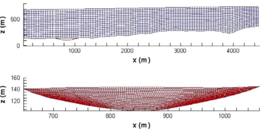
Fig. 8 (upper) shows the space domain chosen for the numerical tests, with top surface elevation and rocky bottom shape taken from measured data. The reference system is chosen so that z = 0 m corresponds to altitude 0 m a.s.l. The vertical boundary at right side is set close to the ice divide, whereas, through the vertical boundary at left, ice flows out. The top boundary corresponds to the atmosphere/icefield interface and the bottom boundary corresponds to the rocky ground except for the flat horizontal portion, where the icefield faces the conjectured subglacial lake whose curved red-colored bottom profile is visible underneath.

The ratio of lake top boundary length over average icefield thickness is about 0.7, that is rather small, so the two-dimensional reduction of ice flow over the lake is admissible (see discussion on the dynamical boundary condition for ice at the lake interface in Section 2.2.1).

506000 508000 510000 512000 514000 51600^ 518000 520000

Fig. 7. Numerical simulation of icefield flow (by ELMER code): ice velocity field (m/yr) at top surface.

•p 500

N

0

I nnn 2000 3000 4000

x(m)

160

"g 140

17 120

700 800 900 1000

x(m)

Fig. 8. Icefield (upper) and subglacial lake (lower) space domain and prototypical finite volume grid.

4.3. Simulation plan for the conjecture check

Relying on the above assumptions and physical and geographical data, we have developed several numerical simulations including the description of the unsteady icefield dynamics with fixed experimental thermal field on a space domain with fixed measured top boundary, of the unsteady subglacial lake dynamics and thermo-dynamics on a guessed space domain and of the unsteady ice/water interface. The mathematical modeling has been reduced in order to incorporate a priori reference data: in particular ice top surface elevation and temperature profile are kept fixed, whereas the remaining variables, evolving in time, are forced to adapt to them. The check of the likelihood of the subglacial lake can be done by pushing time integration forward in order to seek stabilization: if a steady numerical solution with water in the subglacial basin will be reached, then such a lake results 'consistent' - within the adopted mathematical modeling - with estimated data and its real existence depends on the effective presence of the icefield bed depression. In that case a seismic survey would be justified as further investigation.

5. Numerical results

In present paper we develop numerical simulations aimed at tuning the numerical and physical parameters and doing a sensitivity study upon the icefield composition and lake depth. The final results on the check of the likelihood of the subgla-cial lake at Amundsenisen are subject of the next paper [32].

5.1. Icefield space mesh refinement analysis

Before starting the experimentation of the numerical model of the icefield, we have still to fix some parameters. The icefield section for numerical simulation has been chosen along a quasi rectilinear flow-line where ice moves towards an outlet, sliding on the bedrock. Along with this, the Weertman-type sliding condition has been adopted as dynamical boundary condition to ice equations at the icefield bottom (extension of this condition to icefield/lake interface has been jus-tified in Section 2.2.1).

In formula (9), we have done this choices: (p,q) = (1,1) and Nb = p¡gAzav (with Azav average icefield thickness, normal

stress is approximated with ice hydrostatic pressure); the value Q, = 1CT9 has been the best one allowed by the numerical model when it has been challenged to approach the measured value of ice top surface velocity. Commenting on the choice of Q, and on the estimation of the normal stress Nb, Paterson [5] points out that the uncertainty on one of the two quantities

can be overcome by tuning appropriately the other one; more precise evaluations of Nb is out of the scope of this paper.

Due to the heaviness of the numerical simulation, then, we have developed a mesh refinement analysis only for cold ice (see formula ( 1')), assuming that, limited to this issue, considerations may be extended also to temperate ice constitutive relation. Space meshes made of quadrilateral elements have been considered, the tested sizes were: 101 x 16, 151 x 21, 201 x 31, 301 x 46 and 401 x 61.

At time t = 0 d, the ice velocity field has been taken from the fully developed numerical solution obtained with the 3D ELMER code (see Section 4.2. Geographical setting and geometrical reduction). With each grid the simulation has been pushed to time t = 500 d and ice velocity fields have been compared. The results are represented in Fig. 9 with the profile of the horizontal velocity at the vertical outlet of the icefield: convergence appears quite slow, though a trend towards con-vergence is apparent between the finest mesh and the grid 301 x 46. Due to the necessity to limit the computational effort, we have chosen this mesh for the whole following experimentation. With this space mesh maximum time step allowed for integration of the icefield equations has been At, = 0.5d.

5.2. Tuning the eddy viscosity and thermal diffusion coefficients

It is expected that lake water flows into one or more convective cells as result of the icefield driving action at the interface and of the geothermal heating at the bottom.

The LES approach to the lake description (see equations (12) and (15)) leaves the modeler several degrees of freedom that have to be saturated: the choice of the lake space mesh, of the coefficient vectors AM and AH (called EVC and EDC from here

on) and of the kinematical wall boundary condition.

The choice of the space mesh size has obvious implications on the computing effort; the extension of the dynamical and thermo-dynamical vortical structures, 'eddies', described by the model, depends on it while leaving the effect of the subgrid scales of motion to be modeled through the EVC and EDC. The chosen lake finite volume mesh is made of quadrilateral ele-ments drawn by introducing a rectangular mesh on the curvilinear rectangle resulting by properly fixing two points on the lake bottom curve as it is exemplified in Fig. 8 (lower). The size of the adopted space mesh is 113 x 31, with local logarithmic refinement in the neighborhood of the ice/water interface. Actually, comparing results on uniform grid versus results on

300 400 500 600 700

z(m)

locally refined grid leads to the conclusion that, for a satisfactory representation of the phase transition process and heat transfer between the phases, local treatment is mandatory in place of uniform finer meshes that would be computationally too expensive. With the adopted grid the minimum space step in the z direction is Azmin = 0.15 m, that is very fine in the context of oceanographic simulations. Maximum time step allowed for numerical time integration of the lake equations results Atw = 7.2 min.

At paragraph 2.2.1 we have already discussed the possibility to change the no-slip boundary condition to the free-slip one at the lake bottom within the LES formulation. Results obtained with both conditions are compared hereafter.

Finally, the tuning of the EVC and EDC has been accomplished versus target values of the velocity and temperature fields amounting respectively to 0(1 mm/s) and I s Tm(pph) + 3 (to 4) K, being pph, the hydrostatic pressure value at the ice/water

phase front. The lack of any (even local) measured data leads us to rely on published numerical simulation results of inves-tigated subglacial lakes, such as Vostok and Concordia Lakes in Antarctica. In fact these lakes exhibit evident differences with our study case, for this reason we stress that those evaluations are used, here, just to extrapolate the order of magnitude of velocity and temperature fields. Eventually, during final test, along with time integration, numerical solution will adjust to fit present geographical and physical setting.

Now we comment, briefly, on the data in Table 1 from this experimentation, where initial values of EVC and EDC (first row) are taken from Thoma et al. [12], and the following ones are adjusted towards reaching the targets of Tmax and Velmax;

in particular the values A" = 1CT4, A" = 1CT5 and Pr„ = 10, out of Table 1, are kept fixed. In order to understand the extent of the reduction introduced by the LES formulation, it is worth to compare the value of the coefficients A"v with the value of

the exact kinematical viscosity of water at T= 273.15 K, that is v = 1.79 • 10~6 m2/s: LES coefficients are significantly larger as they incorporate the effect of subgrid scale vortices on the surrounding flow in terms of increased viscosity. Moreover the order of magnitude of the coefficients with 'horizontal' impact results higher than the one of 'vertical' impact coefficients as horizontal grid is relatively coarser.

The first set of results, called Bl, is obtained with initial flow at rest and temperature profile slightly increasing from bot-tom to top. This surprising, though physically consistent, temperature distribution (lake colder than icefield) is possible due to the decrease of melting point temperature with pressure (see (3)) which implies that, at lake bottom, its value is lower than at icefield/lake interface. About the results we can see that only those ones reported at the two final rows are compat-ible with liquid phase of water or its metastable state but maximum value of velocity components, Velmax, appears too low.

On the other hand, no slip condition was imposed at the lake bottom and, with the chosen space grid, only with large values of the viscosity coefficient, A", computation is successful. The second set of results, B2, was obtained by initializing each test with the results computed at 5000 time steps with the set of EVC and EDC above in the list and adopted at the previous test.

Table 1

Data and results of numerical tests for tuning EVC and EDC (adopted parameter set in the last row).

Pr„ <(K) Ve/max (mm/s)

Bl-at bottom, no-slip (I.e.: flow at rest, T linear profile T_m(pb) €. T €. Tm(pph))

50 9 70

100 250 300

B2- at bottom, no-slip (I.C.: solution at r =

300 250 200 190 180

B3-at bottom, no-slip (I.C.: solution at t =

300 545.45 250 454.54 200 363.63 150 272.72 50 90.90 35 63.63

B4- at bottom, free-slip (I.C.: solution at t

300 545.45 250 454.54 350 636.36 400 727.27

5000 At based

5.55 7.77 11.11 22.22 33.33

on previous EVC set)

33.33 27.77 22.22 21.11 20

5000 At based on previous EVC set)

0.55 0.55 0.55 0.55 0.55 0.55

= 5000 A t based on previous EVC set) 0.55

" " "

B5- at bottom, free-slip (I.C.: solution at t = 10,000 At based on B3 EVC set)

35 63.63 15 27.27 5 9.09 0.55 " " NAN Inconsistent Inconsistent 272.66 274.35 274.35 274.18 273.93 273.35 273.2 273.03 Inconsistent Inconsistent Inconsistent Inconsistent 272.8 (r = 30,000Ar)

284(r=13,000Ar) 288.3 (r=18,000Ar) 287.4 (r=18,000Ar) 287(r = 22,000Ar)

272.82 (r = 40,000Ar) 272.90 (r = 60,000Ar) 272.94 (r = 90,000Ar)

In this way, by decreasing the value of A™, a too modest increase of Velmax was obtained together with a slight decrease of

temperature (towards metastable state of water).

The third set of results, B3, was computed with the same procedure as B2, starting with the last result and parameter set in the list B^ and successively decreasing either A" (as in B2) and A" in order to keep fixed the horizontal Prandtl number Prh = 0.55, a considerably lower value compared to tests B} and B2. Just with the last set of parameter values, compatible results with proposed target are obtained, though lake temperature appears still too low; for this test, simulation has been pushed forward to t = 30,000 At.

The fourth set of trials, B4, was obtained by changing the no-slip condition at lake bottom into free-slip, keeping fixed both the values of the Prandtl number and starting from the first set of parameter values used in B3. Here, each test has been pushed forward longer than in previous sets of runs, up to the time instants specified in parenthesis beside the temperature values, in order to let the system state develop further. Finally, it appears that the target order of magnitude of velocity is caught but temperature value appears too high.

The first trial of the last set of tests, B5, which is based on the same choice of boundary conditions as in B4, has been ini-tialized with the result of the last test in the set B3, characterized by the lower value of eddy viscosity coefficients". Prandtl numbers are kept as in B4 and the value oí A" is progressively decreased according to A" and keeping Prh = 0.55. Simulations are pushed forward longer than in B4 to reach the time indicated beside the temperature value.

Finally, we have selected the last pattern of boundary conditions and parameter values as the most adequate for the key sperimentation of this work.

5.3. Study of the impact of snow andfirn layers and of lake bottom length

We have tested the sensitivity of the system to the presence of snow and firn layers on the upper region of the icefield in order to check if, within present investigation, it is possible to neglect them.

We have developed simulations only with temperate ice (test case A) and with firn layer (test case B) and with firn and snow layers (test case C); in each case icefield thickness has been kept unchanged.

In addition to density and temperature measured profiles previously introduced in Section 4.1. Physical assumptions, firn and snow have been characterized also through water content. Actually constant water content, W=0.33%, has been assumed for the case of whole temperate icefield combined with Duval's flow rate function (4). For the physical similarities of Amundsenisen Icefield and King George Island ice cap, Breuer et al.'s formula (5), for water content as a function of depth, and associated formulas (6) and (7), for the flow rate function, have been adopted when firn and snow have been included. Influence of temperature on effective viscosity is also represented in (6).

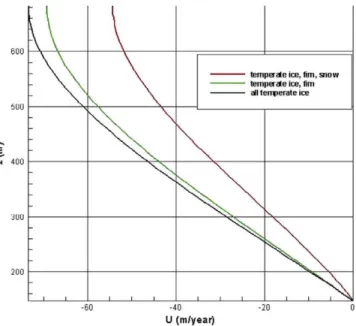
The initial ice velocity field has been taken from the fully developed ELMER code solution (see Section 5.1. Icefield space mesh refinement analysis). In Fig. 10, the graph of the numerical horizontal velocity at the icefield outlet, after 500 days of simulated time, is drawn for each one of the three cases: it results that the relative difference between the top surface values in cases A and C and in cases B and C is quite significant, 0.46 and 0.32 respectively, so we conclude that both snow and firn layers are critical for icefield dynamics and for present investigation.

600

500

M" 400

J LI LI

200

-60 -40 -20 0 U (m/year)

Fig. 10. Icefield horizontal velocity profiles at the outlet, t = 500 d.

\ \

- \

\

\ \

\ \

-"

-- , ,

v \ \

tempérale ¡ce, lim

J

"

'infiérate ice

We show in Fig. 11 the iso-surfaces of the horizontal velocity field in the case C; particle tracks departing from ice divide and running towards the icefield outlet are also visible.

In Fig. 12, imposed water content distribution for test cases B and C is represented.

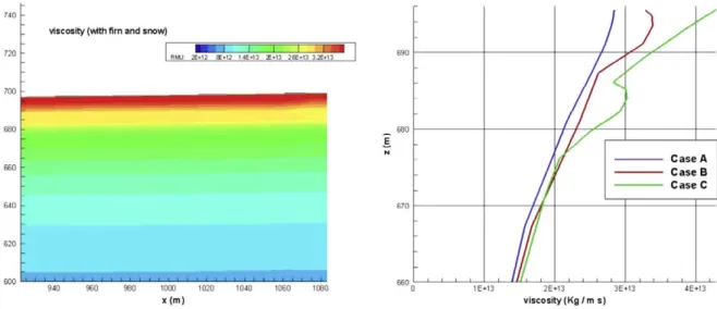
Different values of the effective viscosity at the icefield upper layer are computed and these ones are responsible for dif-ferent ice dynamical response: in Fig. 13 zoomed on the ice upper layer, enhanced increase of the effective viscosity at increasing altitude is clearly visible from iso-surfaces of test case C (left) and from the vertical profiles above the conjectured lake either for test cases B and C (right). In particular, for test case B, effective viscosity curve has a bump in correspondence of firn colder layer; the same bump is clearly visible also for test case C, where a further increase is obtained above, in cor-respondence of snow at lower temperature.

In both the cases B and C, the bumpy profile represents the nonlinear effect of the combined contribution of water content and temperature to the flow rate function in the range of temperature [-2 °C, 0 °C] (see (6)).

U: -76 -70 -65-60 -56 -60-45 -40-36 -30 -25 -20 -15 -10 -5 U (m/year)

2000 3000

x ( m )

Fig. 11. Icefield horizontal velocity iso-surfaces, at time r = 500 d (case C).

1000

i-W3: 0 0.5 0.7 1.2 1.7

•

4 J [I

_l I I I I I I I I I I I I I I I I I I I I L

1000 2000 3000

x ( m )

4000

Fig. 12. Ice water content according to Breuer et al.'s formula (5) (cases B and C).

viscosity (with firn and snow)

^ I I I I • | RMU 2E*12 EE.12 1 4E«13 2E.13 26E.13 3 2E-13

'LIU

N

560

•j-lij

620

-.

-_

-"

"

1

y

Case A Case B

940 960 980 1000 1020 1040 1060 1080 x ( m )

2E*13 3E+13 viscosity (Kg / m s)

In test case A, velocity gradients, that are dominant compared to feeble temperature increase, induce an increase of effec-tive viscosity as well, though much weaker and quasi linear.

For the sake of confidence in our numerical results, we have checked ice local mass conservation: in Fig. 14, the profiles of V • ü along two inner horizontal coordinate lines are drawn within the top half region and the bottom half one. We observe that the numerical residual divergence of u amounts to K.2. • 1CT2 y_ 1 at the largest, a result that we judge satisfactory in this context.

Effects of the inclusion of the firn and snow layers are perceived also in the subglacial lake as it can be seen in Fig. 15, by comparing the thermal field for tests A and C at time t = 500 d: including firn and snow layers (bottom), lake water reaches slightly higher temperature values and, though still lower than Im(p), this is relevant to the aim of checking the compatibility of the existence of the lake which requires metastability be overcome.

Firn and snow layers carry out an insulating action on the system below (ice and lake), so that dispersion of the geother-mal heat from the icefield/lake system is limited, preserving temperate ice, indirectly contributing to melting at the icefield bottom and to increasing lake water temperature; actually, especially firn and snow, interfacing air, do exchange heat with it. Even if the equation for energy balance is not included in present ice modeling, effects of the presence of firn and snow layers are obtained in our simulation by acquiring measured temperature and density profiles, together with appropriate flow rate and water content functions. These ones drive ice dynamics (through effective viscosity) and thermo-dynamics (influencing the value of Im(p)), and, through them, influence also lake water dynamics and thermo-dynamics (by means of the dynamical and thermal boundary conditions and the Stefan condition at the interface).

0 0 6

0.05

-0.03 0.02

001

0.06 0.05

0.03 0.02

0.01

1000 2000 3000 4000

Fig. 14. Residual discrete divergence of ü along longitudinal discrete coordinate lines at top-mid region (left) and at bottom-mid region (right), time

r = 500d (case C).

N 120

,•'00 800 900

x ( m )

1000

160

1 I I

TLV 272.5 272 54 272 •:... ..'_'._ - , 6 6 272.7 272.74

140 120

800 900

x ( m )

As mentioned earlier, the depth of the lake has been simply guessed; on the other hand we understand that a lake with longer bottom profile allows a larger amount of geothermal heat to enter the basin.

Then, we have developed a simulation also with a 20% deeper lake. In Fig. 16, the temperature iso-surfaces with stream-lines are shown at time t = 500 d and, according to expectation, a certain, though weak, enhancement of the thermal field can be observed in comparison with plots in Fig. 15.

Pushing the last simulation forward in time, we have observed that the trend of lake water to overcome metastability and allow the subglacial lake formation shows better off as it can be seen from the thermal iso-surfaces picture at t = 5000 d in Fig. 17.

It is worth to comment briefly on the lake water flow. Here, the particle tracks show clearly that the main vortex rotates in opposition to the driving action of the sliding upper icefield. This is an effect of buoyancy at early stage of simulation (see tuning tests for EVC and EDC, results set Bl in Section 5.2): as, in the vicinity of melting point, water density increases with temperature, the assigned initial increasing thermal (and density) profile is responsible of the onset of clockwise convection.

B00 900

x(m)

Fig. 16. Lake temperature iso-surfaces and streamlines, time t = 500 d (case C, deeper subglacial lake).

TLV 272.45 272.5 27255

1

1

1

1

x(m)

Fig. 17. Lake temperature iso-surfaces and particle tracks, time t = 5000 d (case C, deeper subglacial lake).

140

130

120

110

100

.

! -1.5

U (mm/sec)

-0.5 0 0.5 1 1.5 :

U

Moreover, by looking at streamlines in Fig. 15 we notice that, in test C, main vortex loses the central position, hold in test A: this corresponds to the observed slow down of the icefield motion that allows convection, supported by the geothermal heating, to gain strength. This trend is more evident in Fig 17 for test C with deeper lake due to the increase of geothermal heat entering the cavity.

Momentum transfer from ice to water is, anyway, perceived on top of the lake as it is shown in Fig. 18 for the last test, where the midline vertical profile of the horizontal velocity component appears hold back in the vicinity of interface.

6. Conclusions

We have presented a mathematical numerical model for the description of the dynamical and thermo-dynamical evolu-tion of a system consisting of a grounded icefield and a subglacial lake laying in a bed depression. Glen's law (n = 3) is adopted as constitutive equation of ice and Large Eddy Simulation reduction is applied to lake thermo-hydrodynamics equa-tions. The description of the ice/water phase change process is included in the model. We have approached the solution of the partial differential system with a finite volumes technique and built up a numerical procedure suitable for checking the plausibility of the existence of the subglacial lake. Then we have introduced the study case located at the Amundsenisen Pla-teau (Svalbard) where a subglacial lake is conjectured. This is an accumulation area and the icefield is temperate. Physical and geometrical data from recent field campaigns [10] are taken into account.

Starting from the observation that, according to last decades records, average ice elevation variation may be assumed negligible [29], we have considered reasonable to assume that, at the Amundsenisen Plateau, also other relevant icefield characteristics should not have undergone drastic changes of annual average values during the same time span. So we have adopted the temperature and density profiles of the firn layer measured by Zagorodnov et al. [30] and the average air tem-perature data provided by Hornsund meteorological station and built up a numerical test aimed to check if the conjectured subglacial lake is dynamically and thermo-dynamically compatible with such a data pattern.

Prior to choosing the space grid for simulation we have developed a numerical mesh refinement analysis and then, we have analyzed the sensitivity of the system versus the presence of snow and firn on top of the icefield. At this purpose we have compared two different phenomenological estimates of the water content and flow rate functions, namely, by Duval [16] and by Breuer et al. [17]; numerical solutions appear significantly sensible to local water content variations. The con-tribution of firn and snow to the dynamics and thermo-dynamics of the system is shown to be non-negligible as it is critical for ice flow and for overcoming the typical metastable state of temperate ice with consequent appearance of water in the subglacial cavity.

Consistently with the specialized literature (e.g. Siegert [4]), numerical results point out also that lake cavity depth (or, better, its bottom surface area) is critical for the existence of the lake as the amount of geothermal heat entering the cavity is directly linked to it.

We want to stress that the phenomenological law of water content, taken from Breuer et al., though related to a set of environmental parameters values close to those of the present study case, does not describe dynamically the effect of strain heating due to the specific icefield motion in terms of internal water production and ice effective viscosity. In the next paper [32], an extension of the present model that overcomes this limitation is presented, related numerical results are discussed and the numerical assessment of the likelihood of the subglacial lake is also completed.

Acknowledgements

The authors acknowledge the ESFERANET Polar Climate Consortium for founding the transnational project SvalGlac -Sensitivity of Svalbard Glaciers to Climate Change (2010-2013); presented results are part of its accomplishments. In par-ticular the national agencies supporting the authors are the following: Piano Nazionale Ricerca Antartide (PNRA) (Mansutti), Ministerio de Ciencia e Innovación (MICINN) (Otero) and Narodowe Centrum Badañ i Rozwoju National (NCBiR) (Glowacki). Mansutti thanks Dr. A. Forieri for sharing his on-field experience about subglacial lakes in Antarctica and is grateful to Prof. F.J. Navarro for his expert advice on glaciological issues and his comments for the improvement of the paper.

References

[ 1 ] M.H. Carr, M.J.S. Bel ton, C.R. Chapman, M.E. Davies, P. Geissler, R. Greenberg, A.S. McEwen, B.R Tufts, R. Greeley, R Sullivan, J.W. Head, R.T. Pappalardo, K.P. Klaasen, T.V. Johnson, J. Kaufman, D. Senske, J. Moore, G. Neukum, G. Schubert, J.A. Burns, P. Thomas, J. Veverka, Evidence for a subsurface ocean on Europa, Nature 391 (1998) 363-365.

[2] G. Mitri, A.P. Showman, Convective-conductive transitions and sensitivity of a converting ice shell to perturbations in heat flux and tidal-heating rate: implications for Europa, Icarus 177 (2005) 447-460.

[3] A. Wright, M. Siegert, A fourth inventory of Antarctic subglacial lakes, Antarct. Sci. 24 (2012) 659-664. [4] M.J. Siegert, Antarctic subglacial lakes, Earth Sci. Rev. 50 (1-2) (2000) 29-50.

[5] W.S.B. Paterson, The Physics of Glaciers, Butterworth-Heinemann, Elsevier Science, 2006.

¡6] W. Miller, S. Succi, D. Mansutti, A lattice-Boltzmann model for anisotropic liquid/solid phase transition, Phys. Rev. Lett. 86 (2001) 3578-3581. ¡7] M.M. Cerimele, D. Mansutti, F. Pistella, 'Numerical modelling of liquid/solid phase transitions. Analysis of a gallium melting test', Comput. Fluids 31

(2002) 437-451.

[9] D. Mansutti, E. Bucchignani, M.M. Cerimele, Rayleigh-Benard convection flow with liquid/solid phase transition in a low gravity field, in: M. Rahman, C.A. Brebbia (Eds.), Advances in Fluid Mechanics, vol. 7, 2008, pp. 247-255.

[10] P. Glowacki, A. Glazovsky, Y. Macheret, E. Vasilenko, J. Moore, J.O. Hagen, D. Puczko, M. Grabiec, J. Jania, F.J. Navarro, Dynamics and mass budget of Amundsenisen, Svalbard: interpretation of surface elevation and radar data, IUGG 2007, Perugia, 2007.

[11] R. Greve, H. Blatter, Dynamics of Ice Sheets and Glaciers, Springer-Verlag, Berlin Heidelberg, 2009.

[12] M. Thoma, K. Grosfeld, C. Mayer, 'Modelling mixing and circulation in subglacial Lake Vostok, Antarctica', Ocean Dyn. 57 (2007) 531-540.

[13] M. Thoma, C. Mayer, K. Grosfeld, Sensitivity of subglacial Lake Vostok's flow regime on environmental parameters, Earth Planet. Sci. Lett. 269 (2008) 242-247.

[14] M. Thoma, K. Grosfeld, C. Mayer, F. Pattyn, Interaction between ice sheet dynamics and subglacial lake circulation: a coupled modelling approach,

Cryosphere Discuss. 8 (2009) 805-829.

[15] T. Zwinger, R. Greve, 0. Gagliardini, T. Shiraiwa, M. Lyly, 'A full Stokes-flow thermo-mechanical model for firn and ice applied to the Gorshkov crater glacier, Kamchatka', Ann. Glaciol. 45 (2007) 29-37.

[16] P. Duval, The role of the water content on the creep rate of polycrystalline ice, IAHS 118 (1997) 29-33.

[17] B. Breuer, M.A. Lange, N. Blindow, 'Sensitivity studies on model modifications to assess the dynamics of a temperate ice cap, such as that on King George Island, Antarctica', J. Glaciol. 52 (177) (2006) 235-247.

[18] L. Llyboutry, Physical processes in temperate glaciers, J. Glaciol. 16 (1976) 151-158.

[19] M. Vallon, J.R. Petit, B. Fabre, 'Study of an ice core to the bedrock in the accumulation zone of an Alpine glacier', J. Glaciol. 17 (75) (1976) 13-28.

[20] U. Piomelli, E. Balaras, Wall-layer models for Large Eddy Simulations, Annu. Rev. Fluid Mech. 34 (2002) 349-374.

[21] C.T. Chen, F.J. Mulero, Precise thermodynamic properties for natural waters covering only the limnological range, Limnol. Oceanogr. 31 (3) (1986) 657-662.

[22] R. Kwok, M. Siegert, F. Carsey, Ice motion over Lake Vostok, Antarctica: constrains in inferences regarding the accreted ice, J. Glaciol. 46 (2000) 689-694.

[23] V.R. Voller, C.R. Swaminathan, B.C. Thomas, Fixed grid techniques for phase change problems: a review, Int. J. Numer. Methods Eng. 30 (4) (1990) 875-898.

[24] L. Quartapelle, Numerical Solution of the Incompressible Navier-Stokes Equations, Birkhauser Verlag, Basel, 1993.

[25] E. Bucchignani, An implicit unsteady finite volume formulation for natural convection in a square cavity, Fluid Dyn. Mater. Process. 5(1) (2009) 37-59.

[26] R. Eymard, T. Gallouet, R Herbin, Finite volume methods, in: P.G. CiarletJ.L. Lions (Eds.), Handbook of Numerical Analysis, vol. 7, 2000, pp. 713-1020.

[27] H. Van der Vorst, Bi-CGSTAB, a fast and smoothly converging variant of Bi-CG for the solution of nonsymmetric linear systems, SIAM J. Sci. Stat.

Comput. 13 (2) (1992) 631-644.

[28] G. Golub, C. van Loan, Matrix Computations, The John Hopkins University Press, 1990.

[29] C. Nuth, G. Moholdt, J. Kohler, J.O. Hagen, A. Kaab, 'Svalbard glacier elevation changes and contribution to sea level rise', J. Geophys. Res. 11 (2010) 1-16.

[30] V.S. Zagorodnov, Ldoobrazovanye i glubnoye stroyenie lednikov (Ice formation and inner structure of glaciers), in: V.M. Kotlyakov (Ed.), Glyatsiologiya Spitsbergena, Nauka, Moskva, 1985, pp. 119-147.

[31 ] R.S.W. Van de Wal, R. Mulvaney, E. Isaksson, J.C. Moore, J.F. Pinglot, V.A. Pohiola, M.P.A. Thomassen, 'Reconstruction of the historical temperature trend from measurements in a medium-length borehole on the Lomonosovfonna plateau, Svalbard', Ann. Glaciol. 35 (2002) 371-378.