Second-Best Taxation for a Polluting Monopoly with
Abatement Investment
Guiomar Mart´ın-Herr´ana,∗, Santiago J. Rubiob
aIMUVA and Department of Applied Economics, University of Valladolid, Spain. bDepartment of Economic Analysis and ERI-CES, University of Valencia, Spain.
Abstract
This paper characterizes the optimal tax rule to regulate a polluting monopoly
when the firm has the possibility of investing in an abatement technology and
the environmental damages are caused by a stock pollutant. The optimal policy
is given by the stagewise feedback Stackelberg equilibrium of a dynamic policy
game between a regulator and a monopolist. The regulator playing as the leader
chooses an emission tax to maximize net social welfare, and the monopolist
act-ing as the follower selects the output and the investment in abatement
technol-ogy to maximize profits. We find that the optimal tax has two components. The
first component is negative and equal to the gap between the marginal revenue
and the price caused by the firm market power; the second component is given
by the difference between the social and private shadow prices of the pollution
stock. Considering a linear-quadratic model we show that if marginal
environ-mental damages are constant, the difference between social and private shadow
prices is positive and the optimal policy consists of taxing emissions at a
con-stant rate if the marginal damages are large enough. However, if the marginal
environmental damages are increasing the numerical exercises carried out show
that this difference is negative at the steady state and the optimal policy gives
the firm a subsidy when approaching the steady state regardless of the
impor-tance of the environmental damages. This result is explained by the negative
∗Corresponding author: Facultad de Ciencias Econ´omicas y Empresariales, Avda. Valle
effect that abatement technology accumulation has on the tax. Finally, it can
be pointed out that although both models yield different predictions about the
sign of the optimal policy the dynamics is globally stable for both cases.
Keywords: monopoly, emission tax, pollution stock, abatement capacity,
dynamic games
1. Introduction
The first papers addressing the use of corrective taxes for a polluting monopoly
in a static setting were published by Buchanan (1969) and Barnett (1980).
Buchanan (1969) showed that if marginal damages are low a Pigouvian tax will
lead to a reduction in welfare instead of implementing the efficient outcome. In
fact, if a tax on emissions is used when marginal damages are low, the optimal
tax rate that maximizes net social welfare is negative playing as a subsidy on
production as was pointed out by Barnett (1980).1 Later on, Benchekroun and Long (1998, 2002) extended this analysis in two directions. Firstly, they studied
an oligopolist market and, secondly, they focused on the case of a stock
pollu-tant placing the analysis in a dynamic setting. In the first paper, the authors
show for a linear-quadratic case that there exists a stationary linear tax rule
that leads polluting oligopolists to implement the efficient outcome. The
au-thors propose a three-step procedure. First, they assume that the government
announces at the initial period the tax rule that is applicable to all firms, at
all times. Second, the regulated market equilibrium is calculated as a Markov
perfect Nash equilibrium. Finally, the parameters of the linear tax rule are
computed imposing the output strategy selected by the firms to be equal to the
efficient strategy. The authors show that the equations system defined by this
condition has a unique solution and that the tax increases with the pollution
stock and could be negative for low levels of the stock if there are just a few
firms.2
In Benchekroun and Long’s paper the only way to control emissions is
reduc-1In a very interesting paper Cornes et al. (1986) show for the case of a common-property
resource exploited by an oligopoly that there exists an optimal industry size that implements the efficient outcome as a market equilibrium. Mason and Polasky (1997) analyze this issue in a dynamic setting.
2Im (2002) and Daubanes (2011) also find that optimal taxation of an exhaustible resource
ing production. For this reason, we consider interesting to extend the analysis
of emission taxation to a polluting monopoly to take into account the
possibil-ity of investing in an abatement technology that we assume to be end-of-pipe
type.3 Following a strategic approach, we characterize the optimal tax as an
equilibrium of a dynamic policy game between a regulator that chooses the tax
to maximize net social welfare and a monopolist that selects the output and
the investment in abatement technology to maximize profits. Specifically, we
calculate the stagewise feedback Stackelberg equilibrium (SFSE) of the game
where the regulator is the leader and the monopolist is the follower. The SFSE
gives the leader only a stagewise first-mover advantage that can be interpreted
as the ability of the regulator to commit in the short run.4
In the first part of the paper, we show that the optimal tax has two
com-ponents. The first component is negative and equal to the gap between the
marginal revenue and the price caused by the market power of the firm; whereas
the second component is given by the difference between the social shadow price
of the pollution stock andits private shadow price. The private shadow price
3This end-of-pipe technology mitigates (net) emissions by absorbing pollution at the end
of the production process (e.g., flue gas desulfurization equipment and activated carbon ad-sorption equipment are end-of-pipe technologies). Xepapadeas (1992) addresses the effects of a higher emission tax on the firm’s optimal investment in an abatement technology of this type. More recently, Menezes and Pereira (2017) also assume an end-of-pipe technology to investigate the optimal environmental policy in a dynamic setting when two polluting firms, producing differentiated products, compete in the output marke; and Lambertini at al. (2017) examine the relationship between competition and abatement investment.
4In fact, it is easy to show that if the regulator does not have the ability of short-run
is the price the monopolist associates with the pollution stock because the firm
is aware that the optimal policy selected by the regulator depends on the level
of pollution stock. As the first term is negative, the sign of the optimal policy
could be negative even for a positive difference in the shadow prices.
In order to clarify this issue and investigate the dynamics of the optimal
policy, in the second part of the paper we first solve a linear state (LS) policy
game for which marginal environmental damages are constant; and secondly,
we solve a linear-quadratic (LQ) policy game with increasing marginal
environ-mental damages. With constant marginal damages the optimal policy consists
of taxing emissions at a constant rate provided that marginal damages are large
enough. In this case, we find that the social shadow price of the pollution stock
is positive and increasing with respect to the marginal damages. However, the
monopolist’sshadow price is zero. As the optimal tax does not depend on the
pollution stock, the monopolist’s decision on output (gross emissions) will not
influence the regulator decision on the tax and the monopolist does not give any
value to the pollution stock. On the other hand, the LQ game does not have an
analytical solution but our numerical experiments point out that the optimal
policy at the steady state is a subsidy. We find that for all our simulations
both the social and the private shadow price of pollution stock are positive but
the difference is negative. Thus, the tax becomes a subsidy at the steady state
because its two components are negative. Nevertheless, we may point out that
although both games yield different predictions they present the same type of
dynamics: the steady state is globally stable, i.e. for any initial condition of
the pollution stock and the abatement capacity, all the variables of the model
converge asymptotically to their steady-state values.
In order to have a complete view of the divergence between the private and
social assessment of the state variables by the monopolist and the regulator,
we have also computed the difference in the marginal benefit (value) of the
abatement capacity. This difference is positive at the steady state. Thus, we
may conclude that when a monopoly creates astock externality and the market
stock is larger than themonopolist’sshadow priceof the pollution stockat the
steady state, while the opposite occurs for the marginal values of the abatement
capacity. In this framework, the optimal tax ultimately becomes a subsidy. The
temporal path of the optimal policy is difficult to characterize because it depends
on the initial conditions of the pollution stock and the abatement capacity, but
we can show that it converges to the steady state from above. This means that
the tax becomes a subsidy at some point of time and it is increasing when it
approaches its steady-state value. In fact, we cannot rule out the possibility of
applying a subsidy for the entire time horizon.
This result is explained by the negative effect that the abatement
capac-ity has on the tax. As in Benchekroun and Long’s (1998) paper, we obtain a
stationary linear tax rule with a negative independent term and an increasing
tax with the pollution stock. Without investment in abatement capital, the tax
increases with the pollution stock and if the marginal damages are large enough
the steady-state optimal policy consists of taxing emissions. The optimal policy
is a subsidy when the pollution stock is low, but as the pollution stock converges
to its steady-state value the optimal policy converges to a tax. However, if the
firm invests in an abatement technology, an increase in the abatement capacity
reduces the tax. Our numerical simulations show that in this case as the
pol-lution stock and the abatement capacity tend to their steady-state values the
optimal policy converges to a subsidy. Finally, the negative effect of abatement
capacity accumulation on the tax dominates the positive effect of pollution
ac-cumulation, and therefore, the tax not only decreases but becomes a subsidy
regardless of the importance of marginal damages.
This result plays against the application of an emission tax to regulate a
polluting monopoly when marginal damages are increasing because the optimal
tax simply becomes asubsidy on emissions. Something that is difficult to justify
as an environmental policy. Thus, our analysis suggests that the use of a tax
to control pollution when the market is strongly concentrated as occurs in the
energy markets and in particular in the electricity markets does not seem to be
implement the maximum net social welfare, but also because taxation could not
be an optimal policy in this context and then the use of a tax would have a
negative impact on net social welfareas was already pointed out by Buchanan
(1969) for the case of a flow pollutant.
1.1. Literature Review
The literature addressing the taxation of polluting firms with market power
in a dynamic framework includes only a few papers: Xepapadeas (1992), Kort
(1996), Stimming (1999) Feenstra et al. (2001), Daubanes (2008), Yanese
(2009), and more recently Menezes and Pereira (2017).5 The first four papers
assume that damages are caused by a flow pollutant and focus on the investment
in an abatement technology. For these papers the environmental policy is
ex-ogenously determined and the research assesses the effects of a stricter
environ-mental policy and the comparison of taxes vs emission standards on investment
in abatement technology. In comparison with this literature, our paper
consid-ers that damages are caused by a stock pollutant and the environmental policy
is endogenously determined. Daubanes (2008) extends the analysis developed
by Benchekroun and Long (1998, 2002) to the case of a polluting exhaustible
resource supplied by an oligopoly but the author does not take into account
the possibility of investing in an abatement technology. Maybe, Yanese (2009)
is the first paper where the environmental policy is endogenously determined
although the focus of the research is different from ours and as in Daubanes
(2008) the paper does not consider the possibility of increasing the abatement
capacity. The author examines a non-cooperative policy game between national
governments in a model of international pollution control of a stock pollutant in
which duopolists compete myopically in a third country and expense resources
in abatement activities. Menezes and Pereira (2017) study the dynamic
com-petition between two firms in supply schedules for a stock pollutant using an
5Biglaiser et al. (1995) is a very interesting paper where pollution regulation is examined
abatement technology as the one we assume in this paper. They consider a
model with linear damages and technological spillovers and focus on the
char-acterization of the first-best policy, the mix of emissions tax and R&D subsidy,
assuming that the regulator can commit for the entire temporal horizon and
that the firms’ abatement capital is given by its steady-state value when the
regulator decides the optimal policy. Although our model presents the same
ingredients that those used by these authors, our analysis differs from theirs
in several aspects. We assume that the regulator cannot commit for the entire
temporal horizon and look for time-consistent policy rules. We focus on the
characterization of a second-best tax rule and develop the stability analysis of
the steady state that is not done by Menezes and Pereira (2017), and mainly
we show that with quadratic damages the result obtained for linear damages do
not hold. Thus, to the best of our knowledge, our paper characterizes for the
first time the optimal taxation for a polluting monopoly with a stock pollutant
and investment in abatement technology.
More recently, Wirl (2014) investigated a differential policy game between a
monopoly that provides a clean technology for a polluting competitive industry
and a regulator that uses an emission tax or standard to control a flow
pollu-tant.6 Thus, when the regulator uses a tax, the monopoly is forced to provide
the clean technology at a price equal to the emission tax. For this model, the
Markov perfect Nash equilibria (MPNE) when the regulator applies a tax and
when it uses a standard are compared. The analysis shows that the efficient
solution cannot be implemented using only one instrument, but that the tax
and the standard are equivalent. However, our model presents some differences
with respect to Wirl’s paper. Mainly, we consider the case where damages are
caused by a pollution stock whereas Wirl (2014) analyzes the case of a flow
pollutant. Moreover, we assume that the polluting industry is a monopoly that
6Golombek et al. (2010) consider that the supply of abatement equipment services is
can devote resources directly to abatement activities.
Finally, we would like to comment on the papers by Saltari and Travaglini
(2011) and Karp and Zhang (2012) where both the abatement capital and the
pollution stock are taken into account in the analysis of the firm’s investment
decisions as we do in our paper. Saltari and Travaglini (2011), following the
approach adopted by the previous literature, assume that the emission tax is
exogenously determined and constant. In their model, the pollution stock affects
negatively the production function, and a single price-taker firm has to decide
about the use of a polluting factor and the abatement investment taking as
given the dynamics of the pollution stock that evolves according to a geometric
Brownian motion.7
Karp and Zhang (2012) analyze a two-stage game where in the first stage a
representative firm selects the emissions that maximize its current profits, and in
the second stage the firm and the regulator play a simultaneous non-cooperative
game. In the second stage, the firm decides the level of investment to reduce
abatement costs and the regulator chooses the level of the policy instrument.
They solve the game numerically using a linear-quadratic model for an
appli-cation to climate change. The paper focuses on comparing taxes vs emission
standards. Although the model and strategic approach adopted by Karp and
Zhang (2012) is very similar to the one we follow in this paper, there are some
differences that clearly differentiate our analysis from their analysis. Karp and
Zhang (2012) do abstraction from the type of competition that operates in the
output market, focus on investment to reduce abatement costs and look at a
global environmental problem as the global warming is.
The remainder of the paper is organized as follows. Section 2 presents the
ingredients of the differential game we study in this paper. Section 3
character-izes the optimal policy. In Section 4 a policy game with linear environmental
damages is solved, while in Section 5 it is assumed that damages are given by
7In a more recent paper, Saltari and Travaglini (2017) characterize the optimal growth
a quadratic function. Section 6 offers some concluding remarks and points out
lines for future research.
2. The Model
We consider a monopoly that faces a market demand represented by the
decreasing inverse demand functionP(q(t)) whereq(t) is the output at timet.
The firm produces the output at a constant unit cost c ≥0 and the
produc-tion process generates emissions of pollutants. After an appropriate choice of
measurement units we can say that each unit of output generates one unit of
pol-lution. The emissions can be reduced without declining output if the monopoly
employs an abatement technology that we assume to be end-of-the-pipe type.
For this type of abatement technology the emission function iss(t) =q(t)−y(t)
wherey(t) stands for the installed abatement capacity.8 This capacity can be
increased by w(t) at an increasing cost given by the convex function C(w(t)).
Thus, the dynamics of the abatement capacity is defined by the differential
equation
˙
y(t) =w(t)−δyy(t), y(0) =y0≥0, (1)
whereδy>0 stands for the depreciation rate of the abatement technology. The
focus of the paper is on a stock pollutant that evolves according to the following
differential equation
˙
x(t) =s(t)−δxx(t) =q(t)−y(t)−δxx(t), x(0) =x0≥0, (2)
8We are aware that the linear specification of the emissions function could lead to negative
where x(t) stands for the pollution stock and δx > 0 for the decay rate of
pollution. The environmental damages are given by a function D(x(t)) with
Dx>0 andDxx≥0.
The objective of the firm is to choose output and investment in abatement
capacity in order to maximize the discounted present value of net profits given
by the following expression
max
{q(t),w(t)}
Z ∞
0
e−rt{P(q(t))q(t)−cq(t)−C(w(t))−τ(t)(q(t)−y(t))}dt (3)
subject to differential equations (1) and (2), initial conditions and the usual
non-negativity constraints, where τ(t) stands for the emission tax imposed by
the regulator andr is the time discount rate.9
On the other hand, the environmental regulator chooses the temporal path
of the emission tax with the aim of maximizing net social welfare defined as
the sum of consumer surplus and monopoly net profits plus tax revenues
mi-nus environmental damages subject to differential equations (1) and (2), initial
conditions and the usual non-negativity constraints. As firm tax expenses and
regulator tax revenues cancels out, the dynamic optimization problem for the
regulator can be written as follows
max
{τ(t)}
Z ∞
0
e−rt
Z q
0
P(z(t))dz−cq(t)−C(w(t))−D(x(t))
dt. (4)
Thus, the optimal tax rate is given by the solution to a dynamic policy game
defined by (3), (4) and differential equations (1) and (2).
3. The Reference Differential Game and the Second-Best Emission Tax
As we are interested in characterizing a time-consistent tax, we assume
that the regulator cannot commit in the long run to future taxes and
conse-9As the model is in continuous time we are assuming implicitly that the regulator can
quently we compute a subgame perfect equilibrium in Markov strategies using
the Hamilton-Jacobi-Bellman (HJB) equations. However, it is straightforward
from (4) that if the regulator does not have the ability of short-run
commit-ment its capacity of influencing the monopolist’s decisions vanishes. For this
reason, we assume that output selection occurs after the choice of the tax and
investment.
We assume that the firm is a forward looking agent that realizes of its
dy-namic strategic interdependence with the regulator, because it is aware that the
dynamics of the pollution stock and the abatement capacity that depends on
output (gross emissions) and investment, respectively, will be taken into account
by the regulator to set up the tax. Then the output selection must satisfy the
following HJB equation10
rV(x, y) = max
{q}
P(q)q−cq−C(w)−τ(q−y) +∂V(x, y)
∂x (q−y−δxx)
+∂V(x, y)
∂y (w−δyy)
,
whereV(x, y) stands for the maximum discounted present value of net profits
for the current values,xandy, of the pollution stock and abatement capacity.
From the first-order condition for the maximization of the right-hand side
of the HJB equation, we get
P0q+P =c+τ−∂V
∂x, (5)
where the left-hand side of the condition stands for the marginal revenue of
output and the right-hand side represents the marginal costs. These costs
in-clude the marginal cost of production, the tax and the firm’s shadow price of
pollution stock. The latter is given by the reduction in the discounted present
value of the firm’s profits because of an increase in the pollution stock coming
from an increase in production. Condition (5) implicitly defines the dependence
of the production with respect to the tax and the two state variables: q(τ, x, y).
It is straightforward to see that if the marginal revenue is decreasing, then an
increase in the tax for given values of the stocks leads to a decrease in output.
The reference differential game
Once we have implicitly defined the dependence of the output with respect to
the tax, we can obtain the optimal tax as the solution to the following differential
game
max
{w}
Z ∞
0
e−rt{P(q(τ, x, y))q(τ, x, y)−cq(τ, x, y)−C(w)−τ(q(τ, x, y)−y)}dt,
max
{τ}
Z ∞
0
e−rt
(
Z q(τ,x,y)
0
P(z)dz−cq(τ, x, y)−C(w)−D(x)
)
dt, (6)
subject to
˙
x = q(τ, x, y)−y−δxx, x(0) =x0≥0,
˙
y = w−δyy, y(0) =y0≥0.
We call this differential game, the reference differential game of the model.
Now, expression (6) clearly recognizes the dependence of net social welfare on
the tax because the regulator can influence the market equilibrium through the
imposition of the emission tax.
Next, we calculate the Markov perfect Nash equilibrium (MPNE) of this
reference differential game. The selection of the tax must satisfy the following
HJB equation
rW(x, y) = max
{τ}
(
Z q(τ,x,y)
0
P(z)dz−cq(τ, x, y)−C(w)−D(x)
+∂W(x, y)
∂x (q(τ, x, y)−y−δxx) +
∂W(x, y)
∂y (w−δyy)
,(7)
whereW(x, y) stands for the maximum discounted present value of the net social
welfare for the current values, xand y, of the pollution stock and abatement
capacity.
From the first-order condition for the maximization of the right-hand side
of the HJB equation (7), we get
P(q(τ, x, y)) =c−∂W(x, y)
This condition establishes that the price must be equal to marginal costs that
include the marginal cost of production plus the social shadow price of the
pollution stock.
On the other hand, the selection of the investment in abatement technology
must satisfy the following HJB equation
rV(x, y) = max
{w} {P(q(τ, x, y))q(τ, x, y)−cq(τ, x, y)−C(w)−τ(q(τ, x, y)−y)
+∂V(x, y)
∂x (q(τ, x, y)−y−δxx) +
∂V(x, y)
∂y (w−δyy)
. (9)
Taking into account that the output does not depend on investment we obtain
the following condition
Cw(w) =
∂V(x, y)
∂y . (10)
The left-hand side represents the marginal investment cost. The right-hand side
is the marginal benefit that is given by the increase in the discounted present
value of net profits coming from the increase in the abatement capacity i.e.,
the monopolist’s marginal value of abatement capacity. These two conditions
(8) and (10) implicitly define the optimal strategies for the tax and investment
that characterize the MPNE of the reference differential game. At this point
we should highlight that according to (8) and (10) the optimal policy does not
depend on firm’s investment and the optimal investment does not depend of the
tax what allowsus to conclude that
Proposition 1. The stagewise feedback Stackelberg equilibria (SFSE) of the ref-erence differential game coincide with the MPNE.
The SFSE gives the leader only a stagewise first-mover advantage that can
be interpreted as the ability to commit in the short run. Backward induction
is applied to characterize the equilibrium, substituting the follower’s reaction
function in the leader’s HJB equation, and computing the optimal strategy of
the leader by maximizing the right-hand side of this equation. The reaction
functions given by (8) and (10) are orthogonal and, therefore, directly yield the
depend on investment and, on the other hand, the investment defined by (10)
does not depend on the tax. Thus, the backward induction procedure does not
provide any difference with respect to the optimal strategies that characterize
the MPNE regardless of how is the leader of the reference differential game.11
From the previous result it is straightforward to show that
Corollary 1. The SFSE when the regulator is the leader of the game is consis-tent both in the short run and in the long run.
The short-run consistency is explained by the fact that the two Stackelberg
equilibria of the reference differential game (one when the regulator is the leader
and the other one when it is the follower) coincide. The tax selected by the
reg-ulator when it acts as the leader is the same as the one it chooses when it is the
follower. The equilibrium when the regulator chooses the tax before the
mo-nopolist selects the investment and output is identical to the equilibrium when
the regulator chooses the tax after the monopolist has decided the investment
but before the monopolist selects the output, so that the SFSE is consistent in
the short run. In the long run, the tax is also time consistent because a
sub-game perfect equilibrium in Markov strategies is computed. Notice that when
the regulator is the leader of the reference differential game is also the leader of
the complete differential game defined in the previous section and consequently
Corollary 1 also applies in this case.
Finally, we characterize the tax of the SFSE when the regulator is the leader
of the policy game. Using (5) and (8) we obtain
τ=−(P−M R)−
∂W
∂x −
∂V ∂x
, (11)
whereM Rrepresents the marginal revenue. Thus, the second-best emission tax
is equal to minus the difference between the price and the marginal revenues
11In Rubio (2006) the conditions that explain this coincidence in economic applications of
plus the difference between the social and private valuations of the pollution
stock. The first term reflects the distortion created by the market power of the
firm that leads the firm to value the output at the marginal revenue instead of
valuing it at the market price. The second term reflects the difference between
the social shadow price of the pollution stock,−∂W/∂x, and themonopolist’s
shadow price of the pollution stock, −∂V /∂x. Unfortunately, at this point we
cannot advance in the analysis of the tax components and sign without giving
more structure to our model because at this level of generality the shadow prices
of the pollution stock are given by unknown value function derivatives. For this
reason, in the next two sections, we investigate this issuesolving, first, the policy
game set up in this section when marginal damages are constant; and second,
when they are increasing. We will see that the equilibrium tax rate changes
remarkably with the specification of the environmental damages.
4. The Linear-State (LS) Policy Game
The LS differential game we analyze in this section considers a monopolist
that faces a linear (inverse) demand function given byP =a−q, and operates
with a quadratic investment cost function C(w) = γw2/2, γ > 0. On the other hand, the environmental damages are given by the linear functionD(x) =
dx, d >0.
For this specification of the model, the first-order conditions that
character-ize the SFSE, (5), (8) and (10) can be written as follows
a−2q=c+τ−∂V
∂x, a−q=c−
∂W
∂x , γw=
∂V
∂y,
that yield the optimal strategies for the output and the investment
q=a−c+∂W
∂x , w=
1
γ ∂V
∂y. (12)
Then by difference we can obtain the emissions
s=q−y=a−c−y+∂W
Finally, the resulting tax using the two first conditions is given by the
fol-lowing expression
τ= ∂V
∂x −2
∂W
∂x −(a−c). (14)
This expression can be rewritten as in (11) yielding
τ =−
a−c+∂W
∂x − ∂W ∂x − ∂V ∂x
=−q−
∂W ∂x − ∂V ∂x , (15)
where −q is the difference between the marginal revenue and the price for a
linear demand function, and the second term is the difference between the social
shadow price and thefirm’sshadow price for the pollution stock.
Next, we substitute the production and investment given in (12) in the
reg-ulator’s HJB equation defined by (7) and after rearranging terms the following
nonlinear partial differential equation is obtained
rW = 1
2
a−c+∂W
∂x 2 −1 2γ ∂V ∂y 2
−dx−(y+δxx) ∂W ∂x + 1 γ ∂W ∂y ∂V
∂y−δyy
∂W
∂y .
(16)
Substituting in the monopolist’s HJB equation defined by (9) the following
nonlinear partial differential equation is obtained
rV =
a−c+∂W
∂x
2
−(a−c)y−2y∂W
∂x + 1 2γ ∂V ∂y 2
−δxx ∂V
∂x−δyy
∂V
∂y. (17)
In order to solve this pair of equations, we propose linear representations for
the value functions12
W(x, y) =Drx+Ery+Fr, V(x, y) =Dmx+Emy+Fm,
that yields ∂W/∂x = Dr, ∂W/∂y = Er, ∂V /∂x = Dm, ∂V /∂y = Em with
Dr, Er, Fr, Dm,
EmandFmunknowns to be calculated.
SubstitutingW, ∂W/∂x, ∂W/∂y, V, ∂V /∂x, ∂V /∂yinto (16) and (17) yields
a system of algebraic Riccati equations that presents a unique solution for the
coefficients of the value functions
D∗r=−
d
r+δx
, Er∗=
d
(r+δx)(r+δy) ,
D∗m= 0, Em∗ =2d−(a−c)(r+δx)
(r+δx)(r+δy) .
From these coefficients, we can obtain the optimal strategies defined by
(12).13
Proposition 2. The optimal strategies for the production and investment are
q∗ = a−c− d
r+δx
,
w∗ = 2d−(a−c)(r+δx)
γ(r+δx)(r+δy)
.
The two variables satisfy the non-negativity constraint provided that
1
2(a−c)(r+δx)≤d≤(a−c)(r+δx). (18)
Notice that if d is too large, it does not make sense to produce the good
from an economic perspective because the environmental damages are extremely
huge. Instead ifd is too low, it does not pay to invest in abatement capacity
because the marginal value of abatement capacity, ∂V /∂y =Em∗, is negative. Moreover, it is straightforward to see that an increase in marginal damages
re-duces production and increases investment and consequently leads to a decrease
in the steady-state pollution stock and to an increase in abatement capacity as
can be checked below.
Next, we analyze the dynamics of the state variables given by the following
system of differential equations
˙
x = a−c− d
r+δx
−y−δxx, (19)
˙
y = 2d−(a−c)(r+δx)
γ(r+δx)(r+δy)
−δyy. (20)
13We omit coefficientsF∗
r andFm∗ because they do not affect the results we obtain in this
The steady state of the system is given by
x∗SS = (a−c)(r+δx)(1 + (r+δy)γδy)−d(γδy(r+δy) + 2)
γδxδy(r+δx)(r+δy)
,
ySS∗ = 2d−(a−c)(r+δx)
γδy(r+δx)(r+δy)
,
that yield the following value for the steady-state emissions: s∗SS=q∗−y∗SS =
δxx∗SS.
The steady-state values are non-negative provided that
1
2(a−c)(r+δx)≤d≤
(a−c)(r+δx)(1 + (r+δy)γδy) γδy(r+δy) + 2
, (21)
where the upper bound is lower than the upper bound in (18).
Next, we calculate the characteristic equation of the homogeneous system
corresponding to the two linear first-order differential equations (19) and (20):
λ2+ (δx+δy)λ+δxδy= 0. (22)
The equation has two negative real roots λ1 = −δy and λ2 = −δx and the
general solution for the dynamic system (19) and (20) provided that δy 6=δx
is14
x(t) = y0−ySS
δy−δx
e−δyt+
x0−xSS−
y0−ySS
δy−δx
e−δxt+x
SS, (23)
y(t) = (y0−ySS)e−δyt+ySS. (24)
Thus, we can conclude that
Proposition 3. The system of differential equations for the stock of pollution and abatement capacity has a unique positive steady state provided thatdbelongs
to the interior of interval (21). The steady state is a stable node and is globally
stable, i.e. for any initial (x0, y0) the system converges asymptotically to the
steady state.
As usual the dynamics of the abatement capacity depends on its initial value.
If y0 is lower than the steady-state value, the abatement capacity increases.
14The particular caseδ
However, ify0 is higher than the steady-state value, the opposite occurs. Given
this dynamics we can write the dynamics of emissions as follows
s(t) =q∗−y(t) =q∗−y0e−δyt−(1−e−δyt)y∗SS.
If d belongs to the interval (21), the steady-state emissions are positive and
consequentlyq∗ is larger than y∗SS so that s(t) is positive provided that y0 is
lower than q∗ i.e. that the initial abatement capacity is lower than the gross emissions (production).15
The dynamics of the pollution stock is more complex because it depends
on the relationship between the initial values of the state variables and their
corresponding steady-state values and also on the relationship betweenδx and
δy.The following proposition summarizes the dynamics of the model and Figures
1 and 2 illustrate it. The proof is presented in the Appendix.
Proposition 4. Along the optimal time paths,
• The abatement capacity increases (decreases) if the initial abatement
ca-pacity is lower (larger) than its steady-state value.
• The stock of pollution increases (decreases) if the initial stock is lower
(larger) than its steady-state and the initial point(x0, y0)is above (below)
isocliney˙= 0 and below (above) isoclinex˙ = 0.
• In all other cases, the temporal evolution depends on how characteristic
roots−δx and−δy compare.
– Ifδx≥δy,the pollution stock first increases (decreases) until isocline
˙
x= 0 is reached and decreases (increases) afterwards provided that
y0<(>)ySS∗ .
15As building an abatement capacity has a cost for the firm and no benefit in an unregulated
– Ifδx< δy, the pollution stock first increases (decreases) until isocline
˙
x= 0 is reached and decreases (increases) afterwards provided that
y0 <(>)y∗SS and the initial point is below (above) the straight line
y−y∗
SS = (x−x∗SS)(δy−δx). If this is not the case and the initial
point is above (below) the straight liney−y∗SS = (x−x∗SS)(δy−δx),
the pollution stock is monotonically increasing (decreasing).
Figure 1 shows the phase diagram whenδx≥δy.In this case, the pollution
stock is increasing (decreasing) only when the initial values of the abatement
capacity and pollution stock are below (above) isocline ˙x= 0 and above (below)
isocline ˙y = 0.In the other cases, if the steady-state abatement capacity is lower
(higher) than its steady-state value, the temporal path of the pollution stock has
a maximum (minimum) with a first phase in which the pollution stock increases
(decreases) and a second phase with a decreasing (an increasing) pollution stock.
0 0.1 0.2 0.3 0.4 0.5 0.6 0.7 0.8 0.9 1 0 0.1 0.2 0.3 0.4 0.5 0.6 0.7 0.8 0.9 1
xSS* ySS*
x=0.
y=0. (+) (−)
(−) (+)
0 0.1 0.2 0.3 0.4 0.5 0.6 0.7 0.8 0.9 1 0 0.1 0.2 0.3 0.4 0.5 0.6 0.7 0.8 0.9 1
xSS* ySS*
x=0 . y=0 . (+) (−) (+) (−)
Figure 1: Dynamics of the LS game forδx≥δy(left) andδx< δy(right)
The dynamics of the model forδx< δy is also represented in Figure 1. The
dynamics is richer with six areas that define different temporal paths. Now, the
pollution stock is increasing (decreasing) when the initial values of the
abate-ment capacity and pollution stocks are below (above) isocline ˙x= 0 and above
(below) the straight line that passes through the steady state and has as
capacity can increase or decrease depending on whether the initial value is
be-low or above the steady-state value. If the initial values of the state variables
are in the other two areas, the temporal paths have the same profile than in the
previous case whenδx ≥δy.Finally, it should be pointed out that in this case
if the initial values of state variables are on the straight line with positive slope
that crosses the steady state, the ratio y(t)/x(t) will be constant throughout
the optimal paths that converge to the steady state.
Next, using coefficientD∗r, we can obtain the optimal tax defined by (14).
Proposition 5. The optimal emission tax is
τ∗=−(a−c− d
r+δx
) + d
r+δx
,
which is positive provided that condition (21) is satisfied.
According to expression (15), the first component of the tax is the output
that gives the difference between the marginal revenue and the price for a linear
demand function, and the second component is the difference between the social
shadow price of the pollution stock, −∂W/∂x = −Dr∗ = d/(r+δx), that is
positive, and the private shadow price of the pollution stock, ∂V /∂x = D∗m,
that for constant marginal damages is zero. Thus, the second component of
the emission tax is positive and the sign of the tax depends on the importance
of marginal damages. If these damages are large enough to justify a positive
investment in abatement capacity, the tax is positive and increases with the
marginal damages. In any case, we have that the tax is lower than the social
shadow price of the pollution stock.
On the other hand, the fact that the monopolist’sshadow price is zero
in-dicates that as the tax is constant the optimal decision on output is given by
the maximization condition of current net profits. Thus, for constant marginal
damages the reference differential game can be defined assuming that the firm
myopically selects the output level. However, as we will see in the next section
Finally, the analysis developed in this section shows that although the marginal
damages determine the level of the steady-state values of the different variables
of the model, the dynamics depends on the relationship between the
deprecia-tion rate of the abatement technology and the decay rate of polludeprecia-tion, although
in any case the steady state is globally stable.
5. The Linear-Quadratic (LQ) Policy Game
In this section we assume that environmental damages are quadratic,D(x) =
dx2/2, d >0,implying that marginal damages increase with the pollution stock.
The first-order conditions (5), (8) and (10) that characterize the SFSE do
not depend explicitly on environmental damages. Therefore, the expressions
characterizing the optimal strategies for production, investment and the tax are
the same expressions as those we obtained for the linear policy game. Thus, the
differential equations we obtain substituting the optimal strategies in the HJB
equations are also the same equations as those we obtained for the LS policy
game, except that in (16) the linear term representing the damages must be
substituted by the quadratic term we have just defined.
In order to solve the pair of equations (16) and (17), we propose
linear-quadratic representations for the value functions
V(x, y) = Amx2+Bmy2+Cmxy+Dmx+Emy+Fm,
W(x, y) = Arx2+Bry2+Crxy+Drx+Ery+Fr,
implying
∂V
∂x = 2Amx+Cmy+Dm,
∂V
∂y = 2Bmy+Cmx+Em,
∂W
∂x = 2Arx+Cry+Dr,
∂W
∂y = 2Bry+Crx+Er,
where all the coefficients of the value functions are unknowns to be determined.
SubstitutingW, ∂W/∂x, ∂W/∂y, V, ∂V /∂x, ∂V /∂yinto (16) and (17) yields
a system of algebraic Riccati equations that must hold for everyxandy.Then if
from (12) and (13) the optimal strategies for output, investment and emissions
would be
q(x, y) = a−c+Dr+ 2Arx+Cry, (25)
w(x, y) = 1
γ(Em+Cmx+ 2Bmy), (26)
s(x, y) = q(x, y)−y=a−c+Dr+ 2Arx+ (Cr−1)y. (27)
Finally, using (14) we obtain the optimal strategy for the emission tax16
τ(x, y) =Dm−2Dr−(a−c) + 2(Am−2Ar)x+ (Cm−2Cr)y. (28)
Unfortunately, the system of Riccati equations has not an analytical solution.
For this reason, we develop a numerical exercise to investigate the dynamics
of the system and in particular of the tax when environmental damages are
quadratic.
Numerical exercise
We have solved the model for the following values of the parameters: a =
1000, c = 20, r = 0.05, γ ∈ {2.5,5,10,20}, d ∈ {2.5,5,10,20} and three
combinations ofδxand δy, (δx= 0.05, δy = 0.10), (δx= 0.10, δy= 0.10) and
(δx= 0.10, δy = 0.05),amounting to a total of 48 combinations.
We find that forall combinations of parameter values, the system of Riccati
equations has a unique (globally) stable solution and for all solutions the
dif-ferent terms of the optimal strategies have the same sign given by the following
expressions:17
Output
q(0,0) =a−c+Dr>0,
∂q
∂x = 2Ar<0,
∂q
∂y =Cr>0. (29)
16The derivation of the dynamics of the model has been relegated to the Appendix. 17The system of Ricatti equations and the results of the numerical exercise are presented in
the Appendix.Although we restrict ourselves in this paper to the analysis of linear strategies, we would like to mention that as has been pointed out among others by Rowat (2007) a
Investment
w(0,0) = Em
γ >0,
∂w
∂x =
Cm
γ >0,
∂w
∂y =
2Bm
γ <0.
Emissions
s(0,0) =a−c+Dr>0,
∂s
∂x = 2Ar<0,
∂s
∂y =Cr−1<0.
Tax/subsidy
τ(0,0) =Dm−2Dr−(a−c)<0,
∂τ
∂x = 2(Am−2Ar)>0,
∂τ
∂y =Cm−2Cr<0. (30)
In words, output decreases with the pollution stock, but increases with the
abatement capacity, while the opposite occurs for investment. On the other
hand, emissions are decreasing both with respect to the pollution stock and
with respect to the abatement capacity. Finally, (30) shows that the tax
in-creases with the pollution stock but dein-creases with the abatement capacity.
The numerical analysis also points out that when the two state variables are
zero, the tax becomes a subsidy. To have a better understanding of what drives
the policy rule to give a subsidy when the two state variables are zero, we
ob-serve the second component of the tax given by (15): the difference between
the social shadow price of the pollution stock and the firm’s shadow price of
the pollution stock, because we already know that the first component is always
negative. This difference is defined by the following expression
−
∂W
∂x −
∂V ∂x
=Dm−Dr+ 2(Am−Ar)x+ (Cm−Cr)y, (31)
and our results establish that
Dm−Dr<0, Am−Ar>0, Cm−Cr>0.
Thus, the tax becomes a subsidy forx=y= 0 because thedifference between
the social shadow price of the pollution stock,−∂W(0,0)/∂x=−Dr>0,and
when marginal damages are increasing the firm’s shadow price of pollution stock
is positive. The monopolist is aware of the dependence of the optimal policy
with respect to the evolution of the pollution stock and takes into account this
dependence when it chooses the levels of output and investment associating a
shadow price with the pollution stock equal to the negative effect of an
(in-finitesimal) increase in the pollution stock on the discounted present value of
net profits. According to the optimal policy rule given by (28) and the signs
determined by (30), this negative effect is given by the fact that an increase
in the pollution stock increases (decreases) the tax (subsidy). Then, we can
conclude that the sign of the optimal policy will depend on the initial values
of the pollution stock and the abatement capacity and on the dynamics of the
system. However, for all the numerical simulations we have carried out, the
sign of the optimal policy at the steady state as well as the difference in the
shadow prices are also negative. The tax operates as a subsidy at the steady
state because its two components are negative as it occurs when x = y = 0.
Thus, we find that the divergence between the shadow prices of the pollution
stock strengthens the divergence between the price and the marginal revenue
of output.18 In any case, as established by (15) the subsidy is larger than the
difference between the social and private valuations of the pollution stock.
In order to have a complete view of the divergence between the private and
social assessment of the state variables by the monopolist and the regulator,
we have also computed the difference in the marginal benefit (value) of the
abatement capacity. This difference is given by the following expression
∂W
∂y −
∂V
∂y =Er−Em+ (Cr−Cm)x+ 2(Br−Bm)y.
The numerical analysis establishes that
Er−Em>0, Cr−Cm<0, Br−Bm>0.
18In some cases, the difference in the shadow prices can be positive when the stock increases,
Now, when the initial values of the pollution stock and the abatement capacity
are zero, the regulator’s marginal benefit of the abatement capacity is larger
than the monopolist’s marginal benefit of the abatement capacity. Furthermore,
we also find that this difference is positive at the steady state. Thus we can
conclude that when a monopoly creates a stock externality and the market is
regulated using an emission tax, the private shadow price of the pollution stock
is larger than the social shadow price of the pollution stock at the steady state,
while the opposite occurs for the marginal values of the abatement capacity. In
this framework the optimal tax ultimately becomes a subsidy.
Next, we present the results of the sensitivity analysis of steady-state values
with respect to environmental damages and investment costs, i.e., with respect
to parameters dand γ. For the three combinations of δx and δy we consider
in this numerical exercise, we find that an increase ind reduces the pollution
stock, increases the abatement capacity, negatively affects output, and increases
the subsidy. This positive effect on the subsidy is clearly understood taking into
account that according to the signs given by (30) for the different terms of the
optimal strategy of the tax, the subsidy decreases with the pollution stock and
increases with the abatement capacity. Thus, ifdreduces the pollution stock and
expands the abatement capacity an increase in the subsidy should be expected.
On the other hand, an increase in γ reduces both the pollution stock and the
abatement capacity and negatively affects both output and the subsidy. In this
case, the reduction in the pollution stock increases the subsidy, but the decrease
in the abatement capacity reduces it. The numerical exercise shows that the
net effect is a decrease in the subsidy. The effects on steady-state emissions and
investment are the same that those obtained for the pollution stock and the
abatement capacity.
We close this section analyzing the dynamics of the model. We would want to
point out that for all the cases analyzed in our numerical exercise the following
inequalities apply:
dy dx
x˙=0
=−2Ar−δx
Cr−1
<0, dy
dx
y˙=0
=− Cm
Thus, the slope of isocline ˙x= 0 is negative as in the case with constant marginal
damages, but the slope of isocline ˙y = 0 is positive. Then, if the
combina-tion (x, y) is below (above) isoclines ˙x = 0 and ˙y = 0, then both variables
increase (decrease). In the other cases one variable increases but the other
decreases. Moreover, the coefficients of characteristic equation (B.5) are both
positive yielding two negative roots withλ2< λ1<0 and the dynamics of the
system coincides with the one described in Prop. 5 forδx> δy and represented
in Fig. 1.19 Suppose now that the initial abatement capacity is lower than its
steady-state value. If the initial pollution stock is below isocline ˙x= 0,then the
sign of the initial tax and its dynamics remain undetermined. The sign of the
initial tax depends on the initial values of the state variables and the
dynam-ics could be increasing or decreasing because both the abatement capacity and
the pollution stock are increasing and according to policy rule (28),τ increases
with the pollution stock but decreases with the abatement capacity. However,
once the optimal path of the state variables cuts isocline ˙x = 0 in the phase
diagram of Fig. 1, τ will decrease because the pollution stock will fall and the
abatement capacity will continue to grow. Then given thatτ is negative at the
steady state,τ will necessarily take a negative value when the state variables
approach the steady state. Thus, we cannot reject that during a first phase,
when the pollution stock is increasing, the optimal policy is to tax emissions,
but once it reaches its maximum value and begins to decrease the sign of the
policy will change. If the initial pollution stock is above isocline ˙x= 0 initially a
tax could be applied because the initial pollution stock is high, but as the stock
decreases the tax also decreases and will finally become a subsidy. Nevertheless,
we cannot rule out the possibility of applying a subsidy at allt.20
Finally, we would like to point out that the only relevant change in the
optimal paths when the initial pollution stock is above the isocline x˙ = 0 is
that the initial value forτ is higher than its steady-state value.
19Notice that in the linear modelλ
6. Conclusions
This paper characterizes the optimal policy rule for regulating a polluting
monopoly when the firm has the option of investing in an abatement technology.
We obtain the policy rule by characterizing the stagewise feedback Stackelberg
equilibrium (SFSE) of a dynamic policy game between a regulator and a
monop-olist. The regulator acting as the leader chooses an emission tax to maximize
net social welfare, and the monopolist playing as the follower selects the
out-put and the investment to maximize profits. The SFSE gives the leader only a
first-mover advantage in the short run.
In the first part of the paper, we find that the optimal tax is lower than the
difference between the social and private valuations of the pollution stock. In
order to deepen our understanding of the properties of the tax, in the second
part of the paper, we first solve a linear-state (LS) policy game and, secondly, a
linear-quadratic (LQ) policy game. The results obtained from these two games
are remarkably different although in both cases the steady state is a stable node
and is globally stable. With constant marginal damages the optimal policy
consists of taxing emissions at a constant rate if the marginal damages are
important enough. The difference between the social and private shadow prices
of the pollution stock is positive and larger than the negative component of the
tax, given by the difference between the marginal revenue and the price implied
by the firm’s market power. Unfortunately, the LQ policy game does not have
an analytical solution but a numerical exercise allows us to find some patterns in
the range of parameter values we have considered. The numerical analysis shows
that according to the optimal policy rule the tax increases with the pollution
stock, decreases with the abatement capacity and takes a negative value when
the two state variables are zero. Moreover, we obtain that at the steady state
the two components of the tax are negative. Our numerical simulations show
that the optimal policy is a subsidy at the steady state. This result is the
combination of two forces. First, the monopolist evaluates the output at the
the shadow price that the monopolist associates with the pollution stock is larger
than the shadow price the regulator uses to evaluate the pollution stock. The
optimal temporal path of the optimal policy is difficult to characterize because
it depends, among other things, on the initial conditions. However, we have
found that it converges to the steady state from above, i.e. the optimal policy is
an increasing subsidy when it approaches the steady state. This result is driven
by the negative effect that the accumulation of abatement capacity has on the
tax.
Thus, our analysis establishes that ultimately the optimal environmental
policy consists of subsidizing emissions, although we cannot reject that the
subsidy could be applied for the entire temporal horizon. Obviously, this type
of policy recommendation is difficult to fit from an environmental perspective.
For this reason, it would be very interesting to investigate whether an alternative
policy instrument as an emission standard could work as well as a subsidy in
terms of welfare to regulate a firm with market power that has the possibility of
investing in an abatement technology. This is an issue we point out for future
research. It would be also very interesting to characterize the first-best policy
that implements the efficient outcome. Another extension we would like to
address is to consider other types of abatement technologies different from the
end-of-pipe type in order to check how general is the result we have obtained
in this paper when marginal damages are increasing. Two more issues could
be in the agenda. First, to introduce into the analysis that the abatement
technology can be subject to stochastic innovation or that there is uncertainty
on environmental damages. And, second, it would be also interesting, following
Lambertini et al. (2017), to know how an increase in competition can modify
Appendix A. Proof of Proposition 5
In order to evaluate the dynamics of the pollution stock, we calculate the
first derivative of (23) that can be rearranged as follows
˙
x(t) = (x∗SS−x0)δxe−δxt−
y0−ySS∗
δx−δy
δ
x
eδxt−
δy
eδyt
. (A.1)
To evaluate the sign of this derivative and to know whether the stock is
in-creasing or dein-creasing, we begin studying whether ˙x(t) = 0 has a solution. For
˙
x(t) = 0,expression (A.1) yields
(x∗SS−x0)δx=
y0−ySS∗
δx−δy
δx−δye(δx−δy)t
. (A.2)
On the left-hand side we have a constant and on the right-hand side a function
oftwith the following features: initial value,y0−y∗SS; first derivative,−(y0−
ySS∗ )δye(δx−δy)t; and second derivative,−(y0−ySS∗ )δy(δx−δy)e(δx−δy)t.Thus, the
existence of a solution for this equation depends on the sign of the differences:
x∗SS−x0, y0−y∗SS andδx−δy.
We initiate the analysis consideringδx> δy andy0< y∗SS.In this case, the
function on the right-hand side of (A.2) is an increasing convex function with
a negative initial value, and consequently equation (A.2) has a unique positive
solution provided that (x∗ss−x0)δx > y0−y∗SS. This condition is satisfied if
ySS∗ −δx(x0−x∗SS) < y0,i.e. if vector (x0, y0) is below isocline ˙x= 0. Notice
that isocline ˙x = 0 is a straight line with slope −δx, so that we can write it
as followsy−ySS∗ = −δx(x−x∗SS). Thus, we can conclude that if (x0, y0) is
below isoclines ˙x= ˙y= 0,the stock of pollution first increases until line ˙x= 0
is reached and decreases afterwards. However, if (x0, y0) is below isocline ˙y= 0
but above isocline ˙x= 0,the pollution stock is a monotone decreasing function
of time. Next, we suppose that y0 > ySS∗ . In this case, the function on the
right-hand side of (A.2) is a decreasing concave function with a positive initial
value, and then equation (A.2) has a unique positive solution provided that
(x∗SS −x0)δx < y0−y∗SS, i.e. if vector (x0, y0) is above isocline ˙x= 0. This
decreases until line ˙x= 0 is reached and increases afterwards. But in the case
that (x0, y0) is below isocline ˙x = 0 and above isocline ˙y = 0, the pollution
stock is a monotone increasing function of time. The dynamics we have just
described is represented in Fig. 1 (left) of the main text.
We continue the analysis considering δx < δy and y0 < ySS∗ . In this case,
the right-hand side of (A.2) is an increasing concave function of time with a
negative initial value that converges to the following value
lim
t→+∞
y0−y∗SS
δx−δy
δx−δye(δx−δy)t
=y0−y
∗
SS
δx−δy
δx>0.
In this case, equation (A.2) has a unique positive solution if
y0−y∗SS <(x∗SS−x0)δx<
y0−ySS∗
δx−δy
δx. (A.3)
This condition implies, on the one hand, thaty0< ySS∗ −δx(x0−x∗SS) and, on the
other hand, thaty0< y∗SS+(x0−xSS∗ )(δy−δx) that requires that (x0, y0) is below
isocline ˙x= 0 and below the straight line that passes through the stationary
point (x∗SS, y∗SS) and has as direction vector the eigenvector (1, δy−δx).If this
is the case, the pollution stock first increases until isocline ˙x= 0 is reached and
decreases afterwards. When this condition is not satisfied because the initial
point is above isocline ˙x = 0, the pollution stock is a monotone decreasing
function; while if it is not satisfied because the initial point is above the line
y−y∗SS = (x−xSS∗ )(δy −δx), the pollution stock is a monotone increasing
function.
Next, we suppose that y0 > ySS∗ . When the initial value of the abatement
capacity is larger than its steady-state value, the right-hand side of (A.2) is a
decreasing convex function of time with a positive initial value that converges
to the negative value: (y0−ySS∗ )δx/(δx−δy).Now, equation (A.2) has a unique
positive solution provided that
y0−y∗SS
δx−δy
δx<(x∗SS−x0)δx< y0−ySS∗ .
This condition holds now if (x0, y0) is above isocline ˙x= 0 and liney−ySS∗ =
isocline ˙x = 0 is reached and increases afterwards. When this condition does
not hold, two possibilities arise. In the first possibility the initial point is below
isocline ˙x= 0, and then the pollution stock is a monotone increasing function of
time. In the second possibility the initial point is below the line with direction
vector (1, δy−δx),and in this case the stock of pollution is a monotone decreasing
function of time. Fig. 1 (right) in the main text represents the dynamics we
have just characterized.
Finally, we address the case δx = δy.When the decay rate of the pollution
stock is equal to the depreciation rate of the abatement capacity the two roots
of the characteristic equation (22) are identical and equal toδ.Then, there are
no changes in the solution of differential equation (24) that can be written as
follows
y(t) = (y0−ySS∗ )e−δyt+y∗SS.
However, now the solution for the differential equation of the pollution stock
reads
x(t) =x0e−δt+ (1−e−δt)x∗SS−(y0−y∗SS)te−
δt.
For this solution the first derivative is
˙
x(t) =e−δt((x∗SS−x0)δ−(y0−ySS∗ )(1−tδ)),
so that equation ˙x(t) = 0 has a positive solution provided that the following
expression is positive
t= 1
δ +
x0−x∗SS
y0−ySS∗
. (A.4)
It is obvious that this expression is positive if x0 > x∗SS and y0 > y∗SS or if
x0 < x∗SS and y0 < y∗SS. When x0 > x∗SS and y0 < y∗SS, (A.4) is positive if
y0 < ySS∗ −δ(x0−x∗SS),i.e. if the initial point is below isocline ˙x= 0. When
x0 < x∗SS and y0> ySS∗ ,(A.4) is positive if y0 > ySS∗ −δ(x0−x∗SS), i.e. if the
initial point is above isocline ˙x= 0. Thus, if the initial point is below (above)
isoclines ˙x= ˙y= 0,the pollution stock first increases (decreases) until isocline
˙
the pollution stock increases (decreases) if the initial stock is below (above) its
steady-state value. This is the type of dynamics represented in Fig. 1 (left).
Appendix B. The dynamics of the LQ policy game
Finally, we derive the dynamics of the state variables in terms of the
coeffi-cients of the value functions substituting (25) and (26) in (1) and (2):
˙
x = a−c+Dr+ (2Ar−δx)x+ (Cr−1)y, (B.1)
˙
y = 1
γ(Em+Cmx+ (2Bm−γδy)y). (B.2)
The steady state of the system is given by
xSS =
(Cr−1)Em−(a−c+Dr)(2Bm−γδy)
(2Ar−δx)(2Bm−γδy)−Cm(Cr−1)
, (B.3)
ySS =
Cm(a−c+Dr)−(2Ar−δx)Em
(2Ar−δx)(2Bm−γδy)−Cm(Cr−1)
. (B.4)
In order to study the stability of this dynamic system, we calculate the
characteristic equation of the homogeneous system corresponding to the pair of
linear first-order differential equations (B.1) and (B.2).
λ2+1
γ(γ(δx+δy)−2(γAr+Bm))λ
+1
γ(4ArBm−2(γδyAr+δxBm) +γδxδy−(Cr−1)Cm) = 0.(B.5)
Then ifλ16=λ2,the general solution to the dynamic system is
x(t) = 1
λ1−λ2
((2Ar−δx−λ2)(x0−xSS) + (Cr−1)(y0−ySS))eλ1t
+ 1
λ1−λ2
((λ1−(2Ar−δx))(x0−xSS)−(Cr−1)(y0−ySS))eλ2t+xSS,
y(t) = λ1−(2Ar−δx)
(Cr−1)(λ1−λ2)
((2Ar−δx−λ2) (x0−xSS) + (Cr−1)(y0−ySS))eλ1t
+ λ2−(2Ar−δx) (Cr−1)(λ1−λ2)
((λ1−(2Ar−δx))(x0−xSS)−(Cr−1)(y0−ySS))eλ2t+ySS.
Appendix C. Riccati equations and steady-state values
Substituting the linear-quadratic representations of the value functions in the
system of Riccati equations for the monopolist
8γA2r+Cm2 −2γ(2δx+r)Am= 0, (C.1)
γ(Cr−2)Cr+ 2B2m−γ(2δy+r)Bm= 0, (C.2)
−4Arγ+ 2CmBm+ 4ArCrγ−Cmγ(δx+δy+r) = 0, (C.3)
CmEm+ 4Ar(a−c)γ−(δx+r)γDm+ 4ArγDr= 0, (C.4)
−(a−c)γ−2γDr+2EmBm+2Cr(a−c)γ−γ(δy+r)Em+2CrγDr= 0,(C.5)
Em2 + 2γ(a−c+Dr)
2
−2γrFm= 0, (C.6)
and for the regulator
4γA2r−2γ(2δx+r)Ar−Cm2 −γd+ 2CrCm= 0, (C.7)
γCr2−4B2m−2γCr+ 8BrBm−2γ(2δy+r)Br= 0, (C.8)
2γArCr−2BmCm−2γAr+2BrCm+2CrBm−γ(δy+δx+r)Cr= 0, (C.9)
−2γAr(a−c+Dr) +CmEm+γ(δx+r)Dr−CmEr−CrEm= 0, (C.10)
−γCr(a−c+Dr)+2BmEm+γDr−2BmEr−2BrEm+γ(δy+r)Er= 0, (C.11)
−γ(a−c+Dr)
2
+Em2 −2ErEm+ 2γrFr= 0. (C.12)
This system can be solved sequentially. The first three equations of the two
systems, (C.1)-(C.3) and (C.7)-(C.9), are independent of the rest of equations
and yield the values for coefficientsAm, Bm, Cm, Ar, BrandCr.Given these
values the fourth and fifth equations, (C.4)-(C.5) and (C.10)-(C.11), allow us
to calculate Dm, Em, Dr and Er. Finally the last equation of each system,
(C.6) and (C.12), yieldsFmandFr, respectively. For the 48 cases evaluated in
this numerical exercise, the system of the first three equations gives four real
solutions for each case but in all the cases only one solution is globally stable i.e.,
the roots of the characteristic equation (B.5) are both negative.21 For the other
solutions, the roots are both positive or one positive and the other negative.
Using the solution that is globally stable coefficientsDm, Em, Dr andEr are
21Notice that the coefficients that appear in the characteristic equation are given by this
calculated and the signs (29)-(30) of the optimal strategies terms are determined.
The steady-state values for the pollution stock and the abatement capacity are
obtained calculating the stationary point of the dynamic system (B.1)-(B.2)
and finally substituting in the optimal strategies, the steady-state values for
production and the tax are derived.22 Next tables show the steady-state values
for these variables for two combinations of depreciation rates (δx= 0.05, δy =
0.10) and (δx = 0.10, δy = 0.05). We omit the values for the combination
(δx = 0.10, δy = 0.10) to save space. Nevertheless, they are available from the
authors upon request.
d/γ 2.5 5.0 10 20
2.5 102.8,477.0 81.3,469.2 64.2,453.5 51.2,424.3
5.0 54.7,478.9 42.7,470.7 33.3,454.6 26.3,425.2
10 28.8,479.9 22.2,471.5 17.1,455.2 13.4,425.9
20 15.0,480.4 11.4,471.9 8.8,455.5 6.8,425.9
Table C.1: Pollution stock and abatement capital (δx= 0.05, δy= 0.10)
d/γ 2.5 5.0 10 20
2.5 113.0,478.0 92.4,476.8 76.1,472.2 63.5,461.9
5.0 60.2,482.3 48.5,480.3 39.5,475.1 32.7,464.2
10 31.6,484.6 25.2,482.1 20.3,476.5 16.7,465.4
20 16.4,485.7 13.0,483.0 10.4,477.3 8.5,466.1
Table C.2: Pollution stock and abatement capital (δx= 0.10, δy= 0.05)
Using the figures in Tables C.1-C.4, we elaborate the sensitivity analysis
22Observe that at the steady state, the investment is given by w
SS = δyySS and the
emissions bysSS=δxxss.For this reason, we do not find necessary to show these values in
δx= 0.05, δy= 0.1 δx= 0.1, δy= 0.05
d/γ 2.5 5.0 10 20 2.5 5.0 10 20
2.5 482.2 473.3 456.7 426.9 489.3 486.0 479.8 468.2
5.0 481.7 472.9 456.3 426.5 488.3 485.1 479.0 467.5
10 481.4 472.6 456.1 426.3 487.7 484.6 478.6 467.1
20 481.2 472.5 456.0 426.2 487.4 484.3 478.3 466.9
Table C.3: Output
δx= 0.05, δy= 0.1 δx= 0.1, δy = 0.05
d/γ 2.5 5.0 10 20 2.5 5.0 10 20
2.5 1710.1 1329.5 1009.0 730.1 1520.3 1233.1 1000.0 807.7
5.0 1815.7 1393.7 1046.5 750.9 1610.2 1289.7 1034.7 828.5
10 1906.5 1447.2 1076.9 767.5 1688.1 1337.1 1063.0 845.1
20 1981.6 1490.1 1100.7 780.4 1752.7 1375.3 1085.4 858.0
Table C.4: Subsidy
d/γ 2.5 5.0 10 20
2.5 1227.9(71.8) 856.2(64.4) 552.3(54.7) 303.2(41.5)
5.0 1334.0(73.5) 920.8(66.1) 590.2(56.4) 324.4(43.2)
10 1425.2(74.8) 974.6(67.3) 620.8(57.7) 341.2(44.5)
20 1500.4(75.7) 1017.6(68.3) 644.8(58.6) 354.2(45.4)
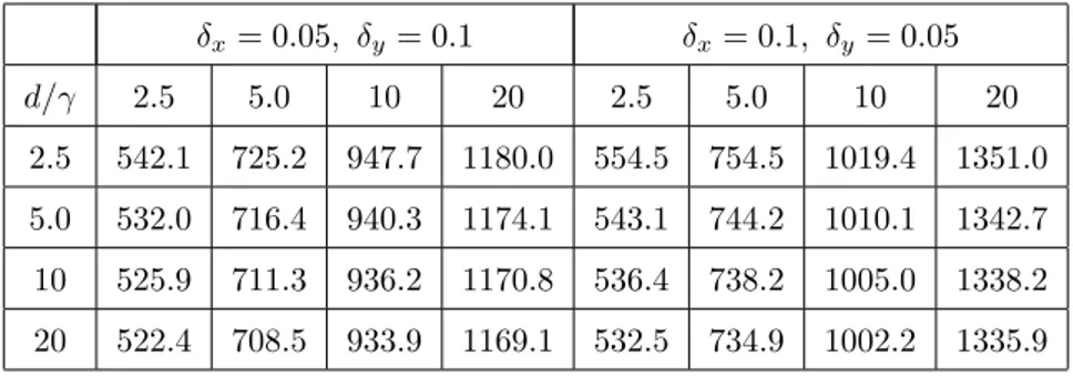
Table C.5: Differences in shadow prices (δx= 0.05, δy= 0.10)
d/γ 2.5 5.0 10 20
2.5 1031.0(67.8) 747.1(60.6) 520.2(52.0) 339.5(42.0)
5.0 1121.9(69.7) 804.5(62.4) 555.7(53.7) 361.0(43.6)
10 1200.3(71.1) 852.5(63.8) 584.5(54.9) 378.0(44.7)
20 1265.3(72.2) 891.0(64.8) 607.0(55.9) 391.1(45.6)