TítuloBayesian estimation of ruin probabilities with heterogeneous and heavy tailed insurance claim size distribution

Texto completo

(1)Bayesian estimation of ruin probabilities with heterogeneous and heavy-tailed insurance claim size distribution M. Concepcion Ausin∗. Hedibert F. Lopes. Department of Mathematics. Graduate School of Business. University of A Coruña, Spain. University of Chicago, USA. mausin@udc.es. hlopes@gsb.uchicago.edu Abstract. This paper describes a Bayesian approach to make inference for risk reserve processes with unknown claim size distribution. A flexible model based on mixtures of Erlang distributions is proposed to approximate the special features frequently observed in insurance claim sizes such as long tails and heterogeneity. A Bayesian density estimation approach for the claim sizes is implemented using reversible jump Markov Chain Monte Carlo methods. An advantage of the considered mixture model is that it belongs to the class of phase-type distributions and then, explicit evaluations of the ruin probabilities are possible. Furthermore, from a statistical point of view, the parametric structure of the mixtures of Erlang distribution offers some advantages compared with the whole over-parameterized family of phase-type distributions. Given the observed claim arrivals and claim sizes, we show how to estimate the ruin probabilities, as a function of the initial capital, and predictive intervals which give a measure of the uncertainty in the estimations. Keywords: Bayesian mixtures; heavy tails; multimodality; phase-type distributions; reversible jump MCMC; risk reserve processes.. 1 Corresponding author. M. Concepción Ausı́n, Departamento de Matemáticas, Facultade de Informática, Campus de Elviña, Universidade da Coruña, 15071 A Coruña, Spain. Tel.: +34 981 167 000 (ext. 1318); fax: + 34 981 167 160. E-mail address: mausin@udc.es Running title: Estimation of ruin probabilities with heterogeneous and large claims. 1.

(2) 1. Introduction. The choice of an appropriate model for the claim sizes among the plethora discussed in the literature is crucial in the analysis of insurance processes. For example, under the presence of large claims, the ruin probability for a given initial capital can be underestimated if an inadequate model is considered for the claim size distribution. One of the most popular families considered to model claim sizes is the class of phase-type (PH) distributions, see e.g. Asmussen (2000) and Rolski et al. (2000), which were introduced in a queueing context by Neuts (1981). Assuming PH distributed claim sizes, it is possible to explicitly evaluate ruin probabilities for different risk models avoiding the use of approximations such as the frequently used Cramér-Lundberg inequality. Furthermore, any positive distribution can be arbitrarily closely approximated by a PH distribution due to the denseness property. Many different fitting methods have been proposed for PH distributions using moment matching methods (Johnson & Taffe, 1991), maximum likelihood estimation (Asmussen et al., 1996) and Bayesian techniques (Bladt et al., 2003). However, it is well known that the whole class of PH distributions is a non-identifiable family because different sets of parameters may lead to the same PH distribution, see e.g. Neuts (1981). This overparameterization can produce problems in fitting algorithms based on observed data, which eventually lead to poor parameter estimates and high computational costs. In order to reduce the number of parameters, two main subsets of PH distributions have been proposed in the literature: the Coxian distributions, see e.g. Faddy (1994), and the mixtures of Erlang distributions, see e.g. Schmickler (1992). These two distribution families are also dense on the positive reals and consequently, can also approximate any positive distribution using a smaller number of parameters. There has been much work on the calculation of ruin probabilities in insurance risk processes with PH claim sizes, see e.g. Asmussen & Rolski (1991), Avram & Usabel (2003), Dickson & Drekic (2004) and Drekic et al. (2004). However, their statistical estimation has received comparatively much less attention. Inference for risk reserve processes and estimation of ruin probabilities have been traditionally carried out using MLE estimation, see Asmussen (2000), and nonparametric inference, see Hipp (1989). Bayesian approach of risk models have received recent interest in the insurance literature, see Cairns (2000) and Bladt et al. (2003). The Bayesian methodology offers a natural way to introduce the inherent parameter and model uncertainty in the estimation of ruin probabilities. Also, predictive distributions of the ruin probabilities can be obtained which are more informative than simple point estimations and allow to construct confidence intervals. Furthermore, it is possible to estimate the probability of having a positive safety loading and directly incorporate this uncertainty in the estimation of the required ruin probability. Finally, it is well. 2.

(3) known that insurance risk models and queueing systems are mathematically very related. Thus, we can make use of the large number of Bayesian approaches for queueing systems existing in the literature, see e.g. Armero & Bayarri (1994), Rios et al. (1998), Wiper (1998), Armero & Conesa (2004) and Ausin et al. (2003, 2004, 2005). In this paper, we present a procedure for Bayesian inference and prediction of the classical compound Poisson process with unknown claim size distribution. We propose a special reparameterization of mixtures of Erlang distributions as a suitable model to approximate the claim size behaviour including the possibility of heterogeneity or extreme values. The dense family of mixtures of Erlang distributions includes simpler models such as the exponential, Erlang and hyperexponential distributions as special cases, and belong to the class of PH distributions. Therefore, given the mixture parameters, explicit expressions of the ruin probabilities can be obtained. Bayesian inference for mixtures of Erlang distributions has been previously considered in Ausin et al. (2004), in the context of queueing systems and using the standard mixture parameterization. This standard formulation require the use of a joint proper prior distribution for the mixture parameters which leads to poor approximations of long-tailed distributions. The new parameterization proposed in this article will allow us to consider an improper prior and develop a straightforward Markov Chain Monte Carlo (MCMC) implementation, obtaining good approximation of both long tails and multimodality with a relatively small number of parameters. This article is organized as follows. In Section 2, we briefly introduce the definition and some properties of the class of PH distributions and the subset of Coxian distributions, including some discussion on the problems with their parameterization. In Section 3, we carry out Bayesian inference for a reparameterization of mixtures of Erlang distributions given a non informative prior and an unknown number of mixture components. In Section 4, we develop Bayesian prediction for the classical compound Poisson process introducing the uncertainty derived from the estimated claim size distribution. We analyze the probability of having a positive safety loading and obtain point estimates and credible intervals for the ruin probabilities. We illustrate the methodology in Section 5 with a variety of simulated claim sizes including long-tails or/and multimodality. We conclude in Section 6 with some discussion and extensions.. 2. Phase-type distributions. A positive distribution is of phase-type (PH) with representation (m, α, T ) , see Neuts (1981), if it represents the distribution of the time to absorption in a Markov jump process with m transient states and one absorbing. 3.

(4) state (state m + 1). Then, the intensity matrix is given by, .   T Q= 0. t0  , 0. where T is a proper m × m subintensity matrix and the column vector of exits rates is t0 = −T e, where e is a column vector of ones. The initial probability vector is (α, αm+1 ) with αe + αm+1 = 1, where α is a 1 × m row vector of probabilities. The distribution function is given by,. F (x) = 1 − α exp {T x} e,. for x > 0,. where exp {T x} is the matrix exponential of T x and the matrix exponential of a matrix A is defined by the X∞ power series exp{A} = Ak /k!. The corresponding density function is given by, k=0. f (x) = α exp {T x} t0 ,. for x > 0.. The simplest phase-type distribution is the exponential density, f (x) = µ exp (−µx) , with representation (m, α, T ) = (1, 1, −µ). Another two classical examples of phase-type distributions are the mixture of Pk exponentials, f (x) = r=1 ωr µr exp {−µr x} , with m = k, α = (ω1 , ..., ωk ) and T = diag (−µ1 , ..., −µk ), and the Erlang density, ν. f (x) =. (νµ) ν−1 x exp {−νµx} , Γ (ν). for x > 0,. (1). with m = ν, α = (1, 0, ..., 0) and  −νµ     T =   .  νµ .. .. ... .. −νµ.       νµ   −νµ. .. (2). ν×ν. The whole class of PH distributions is a very versatile family and is dense over the set of positive distributions. Thus, any given positive density can be approximated arbitrarily closely by a PH distribution, see Neuts (1981). But unfortunately, this distribution family is not identifiable as the parameters (m, α, T ) do not determine uniquely one distribution, that is, different PH representations can lead to the same distribution. Also, note that for a given m, the number of free parameters of a phase-type distribution is m2 +m. This over-parameterization will produce instability in the estimation algorithms and difficulties with. 4.

(5) parameter identifiability. Alternatively, a wide sub-class of PH distributions, named Coxian distributions and also called acyclic PH or MGE distributions, has been frequently used in the literature, see e.g. Faddy (1994). The Coxian distribution can be represented by m, α = (α1 , α2 , ..., αm ) and,  −λ  1    T =   .  λ1 .. .. ... .. −λm−1.     ,  λm−1   −λm. (3). where, without loss of generality, it can be assumed that λ1 ≤ λ2 ≤ ... ≤ λm . Note that the number of free parameters in a Coxian distribution is reduced to 2m−1, for each value of m. The Coxian family is also dense and is an appropriate model to approximate long-tailed distributions, see e.g. Horvath and Telek (2000). However, the number of parameters required to capture peaked (platykurtic) density functions is still very large. To illustrate this, suppose we have a data set generated from an Erlang distribution, whose density is given in (1), with parameters ν = 50 and µ = 0.5. Then, if we consider a Coxian distribution to model these data, the estimation of the matrix (3) should be close to the matrix given in (2) with an estimated value for m close to 50. Thus, we should estimate around one hundred parameters (2m − 1) to obtain a good fitting. Thus, the Coxian model requires a large number of parameters to approximate multimodal distributions, and clearly, this problem persists for densities which are simultaneously multimodal and platykurtic. In the next section, we introduce and develop inference for the family of mixtures of Erlang distributions which can capture long-tails, multimodality and/or low kurtosis using a smaller number of parameters.. 3. Model and inference for the claim size distribution. In this paper, we assume that the claim size distribution follows a mixture of Erlang distributions with parameters k, ω = (ω1 , ..., wk ) , µ = (µ1 , ..., µk ) and ν = (ν1 , ..., νk ), whose density function is given by,. f (x | ω, µ, ν) =. k X. ωr Er (x | νr , µr ) ,. for x > 0,. (4). r=1. where. Pk. r=1 ωr. = 1; ωr , µr > 0; νr ∈ N and Er(x | νr , µr ) is the Erlang density function given in (1),. whose mean and variance are given by 1/µr and 1/νr µ2r , respectively, for r = 1, ..., k. Note that under this distribution, each generic claim size, x, is with probability ωr , the sum of νr exponential phases of rate µr . Clearly, the distribution model (4) is a mixture of exponentials when νr = 1, for r = 1, ..., k, and a single Erlang distribution when k = 1. Mixtures of exponentials have been successful in modeling loss data for 5.

(6) actuarial problems, see e.g. Keatinge (1999). A mixture of Erlang distributions is of phase-type as it is a mixture of phase-type distributions, see Neuts £ ¤ Pk (1981). It can be represented with m = r=1 νr ; α = (ω1 , 0, ...0)1×ν1 , ...., (ωk , 0, ..., 0)1×νk and T equal to a block diagonal matrix with k blocks such that each one is of size νr × νr , for r = 1, ..., k, and is given by (2). Although it can be shown that the mixtures of Erlang distributions are a subset of the family of Coxian distributions, see Asmussen (2000), we believe that the flexibility of the Erlang mixture model is practically equivalent to the flexibility of the Coxian family with the advantage of a having more compact parameterization. In practice, we have not found any pattern that can be captured by an Coxian distribution and not by an Erlang mixture using the following Bayesian approach, as will be shown in the examples. Now, we describe a Bayesian density estimation method for the claim size distribution based on the Erlang mixture model, (4). Our objective is to make Bayesian inference for the mixture parameters given a sample of n observed claim sizes, x = {x1 , ..., xn }. Firstly, note that as the mixture model is identifiable up to permutation of the rates, we can assume that,. µ1 ≥ µ2 ≥ ... ≥ µk ,. (5). which is equivalent to assume an increasing order for the means. Then, we can consider the following reparameterization, µr = µ1 τ2 ...τr ,. where 0 < τj ≤ 1, for r, j = 2, ..., k.. This kind of reparameterization has also been considered in Robert & Mengersen (1999) for normal mixtures, in Gruet et al. (1999) for exponential mixtures, and in Ausin et al. (2005) for Coxian distributions. Some of the known advantages of this type of parameterization are the use of noninformative priors and the improvement of the mixing in the MCMC algorithms. We now define a prior distribution for the mixture parameters, (k, ω, µ1 , τ , ν). We assume a flat prior for the number of mixture components, k, for example, a discrete uniform defined on the interval [1, kmax ]. In our examples, we have chosen kmax = 20 which, in practice, is large enough to capture the usual patterns observed in claim size distributions. Using the new reparameterization, it is possible to define the following improper prior distribution for the first rate, f (µ1 ) ∝. 1 . µ1. (6). The choice of this improper prior for µ1 will allow for the approximation of long-tailed distributions as will be shown in the examples. This is because we do not make a strong assumption about the mean of the. 6.

(7) first component and then, the remaining mean components of the mixture will be able to be as large or as small as required. Also note that this improper prior distribution for µ1 will imply an improper joint prior distribution. However, the joint posterior distribution is proper as shown in the Appendix. Note that using the standard parameterization, as in Ausin et al. (2004), it is not possible to use an improper prior for each mixture component rate as it leads to an improper posterior distribution, see e.g. Diebolt & Robert (1994). Conditional on k, we define proper but diffuse prior distributions for the remaining parameters as follows,. ω|k ∼ Dirichlet(φ1 , ..., φk ),. (7). τr |k ∼ Beta(a, b),. (8). for r = 1, ..., k,. νr |k ∼ Geometric(p),. for r = 1, .., k.. (9). In the examples, we have set φr = 1 to give a uniform prior over the weights. Also, we have set a = b = 1 to give a uniform prior over each τr , for r = 1, ..., k. Finally, we assume a not very large prior mean 1/p for νr in order to penalize a large number of phases in the Erlang mixture, for example we have set in the illustrations p = 0.05. In order to simplify the derivation of the conditional posterior distributions, we also introduce the usual missing data formulation for mixtures setups, see e.g. Diebolt & Robert (1994), where a set of latent variables Z1 , ..., Zn are defined such that,. Xi | Zi = r ∼ Er (νr , µr ) ,. Pr (Zi = r | ω, k) = wr ,. for r = 1, ..., k. Thus, the observed data, x = (x1 , ..., xn ) , are completed with a missing data set, z = (z1 , ..., zn ) , indicating the specific mixture components from which the observations are assumed to arise. Now, conditional on k, we can construct an MCMC algorithm to sample from the joint posterior distribution of the mixture parameters. The considered parameterization together with the assumed prior distribution allow for a straightforward implementation of a Gibbs sampling scheme where all the condi-. 7.

(8) tional posterior distributions are explicit. Given k, these conditional distributions are given by,. ω|x, z ∼ Dirichlet(1 + n1 , ..., 1 + nk ), ¶ µ k k r P P Q µ1 |ν, x, z ∼ Gamma nr νr , νr sr τs , s=2 r=1 r=1 Ã j k k P P Q τr |τ−r , ν, x, z ∼ Gamma 1 + nj νj , µ1 νj sj j=r. j=r. ! τs. s=2,s6=j. I0<τr ≤1 ,. (10). νr. f (νr |ω, µ, x, z) ∝. νrnr νr (1 − p) Γ(νr )nr. exp {−νr (sr µr − nr log µr − log pr )} ,. (11). for r = 2, ..., k, , where τ−r = (τ1 , . . . , τr−1 , τr+1 , . . . , τk ), nr is the number of observations assigned to the r-th component and sr and pr are the sum and the product of these observations, respectively. Note that we assume that sr and pr are equal to zero when nr is zero. Observe that the distribution of τr (10) is a truncated gamma density that can be sampled straightforwardly using a rejection sampling method such as the proposed in Phillipe (1997). The conditional posterior distribution of νr (11) is a discrete distribution whose support is the whole set of positive integers. This can also be easily generated if we assume a truncation over a finite interval, 1 ≤ νr ≤ νmax , for r = 1, ..., k. We have found that νmax = 100 is large enough in most practical situations. In order to sample from the posterior distribution of k, we make use of the reversible jump techniques introduced by Green (1995) and, applied for normal mixtures, in Richardson & Green (1997). The reversible jump algorithm is a generalization of the Metropolis Hastings method for variable dimension parameter spaces. Candidate values for the parameters are proposed to allow changing the number of mixture terms from k to k ± 1 and then, these candidates are accepted or rejected with the corresponding probability. We consider the so-called split and combine moves where two consecutive components in the sense of (5) are combined into one mixture component and, to allow reversibility, one mixture component is split into two, respectively. If the r1 -th and r2 -th components are combined into the new r-th component, the parameters are modified such that, w̃r = wr1 + wr2 ,. τ̃r = τr1 τr2 ,. ν̃r = νr2 ,. which implies that the proposed rate for the new component is µ̃r = µr2 . Also, it is considered that µ1 = µ1 τ2 when r1 = 1. For a split move, the parameters of the new r1 -th and r2 -th components are given by, w̃r1 = u1 wr ,. w̃r2 = (1 − u1 )wr ,. τ̃r1 = u2 + τr (1 − u2 ) , ν̃r1 = u3 ,. τ̃r2 =. τr u2 +τr (1−u2 ) ,. ν̃r2 = νr ,. 8.

(9) ³ ´ νr −1 where u1 and u2 are uniform U (0, 1) and (u3 − 1) ∼ B νmax , νmax −1 , a binomial distribution such that E [u3 ] = νr . This split move implies that µ̃r2 = µr . For the case that r = 1, we generate µr1 = µ1 /u2 and τ̃2 = u2 where u2 ∼ U (0, 1). Also, those observations with zi = r are allocated to one of the r1 -th or r2 -th component with probability, ´ ³ ¡ ¢ Pr Z̃i = rj ∝ ω̃rj Er xi | νrj , µrj ,. for j = 1, 2.. Note that these moves have been proposed following Gruet et al. (1999) and are chosen such that the parameters of the remaining mixture components are not modified. Also note that these moves do not preserve in general the mean and variance of X. The acceptance probability of a split move is min {1, A} where, A=. Y ω̃z̃ Er (xi | ν̃z̃ , µ̃z̃ ) ωr (1 − τr ) d i i i ³ L+1 ´ × × , Q ω Er (x | ν , µ ) u ri i r r 2 + τr (1 − u2 ) Pr Z̃i = z̃i q (u3 ) bL zi =r zi =r. when r > 1, where dL and bL are respectively the probabilities of a combine or a split move and q (u3 ) is the probability of having generated u3 from the binomial distribution. Note that the last factor refers to the determinant of Jacobian of the corresponding transformations. The acceptance probability for the reverse combine move can be obtained analogously. Once we have run the MCMC algorithm, we obtain a sample of size J of the posterior distribution of the model parameters, {(k (j) , ω (j) , µ(j) , ν (j) )}Jj=1 , and we can approximate the predictive density of the claim size distribution by the usual Monte Carlo estimation approach, (j). f (x | x) ≈. J k ´ 1 X X (j) ³ ωr Er x | νr(j) , µ(j) . r J j=1 r=1. Note that this Bayesian density estimator is in fact a mixture of. PJ. j=1 k. (j). (12). Erlang distributions terms which. provides a great flexibility to the resulting estimated density. This predictive density do not provide a single “best” Erlang mixture model, but a coherent way of combining results over different Erlang mixture models. Analogously, we can estimate the predictive cumulated distribution function using the incomplete gamma function formula as follows, ³ ´i (j) (j) J X k(j) n o νr(j) −1 ν µ x X r r P 1 F (x | x) = 1 − . ω (j) exp −νr(j) µ(j) r x J j=1 r=1 r i! i=0. (13). Finally, we can also perform inference for the mixture parameters. For example, we can estimate the. 9.

(10) posterior distribution of the number of mixture components by,. Pr (k = r | x) =. 4. o 1 n # j : k (j) = r . J. (14). Bayesian prediction of ruin probabilities. Given an initital capital, u, we are now interested in estimating the ultimate ruin probability of an insurance company which is defined as,. µ ¶ ψ (u) = Pr inf Rt < 0 | R0 = u , t≥0. (15). where {Rt }t≥0 is the risk reserve process describing the reserves of an insurance company and is given by, Rt = u + ct −. Nt P i=1. Ui ,. (16). where c is the premium rate, Nt is the number of claims up to time t and U1 , U2 , ... are the claim sizes. We assume a classical compound Poisson model where Nt is an homogeneous Poisson process with rate λ independent of the claim sizes, which are assumed to be i.i.d. following a mixture of Erlang distributions as described in the previous section. In order that the ruin probability ψ (u) differs from one for each value of the initial capital, u, it is −1. required that the safety loading η is positive, where η = c (λE [U ]). − 1, see e.g. Asmussen (2000). Thus,. in risk theory, the safety loading is usually assumed to be positive which implies that the process tends to plus infinity with probability one and then, the insurance company avoids certain eventual ruin. However, in practice, this condition is not always ensured, that is, it is not always known if the premiums are on average larger that the expected claims. Moreover, there is frequently evidence of a “heavy traffic” in the data which means that on average, the claim sizes are only slightly smaller than the number of claim arrivals per unit time in which case the safety loading is positive and small. Thus, we will not impose the condition η > 0 in our risk model where the claim sizes follow a mixture of Erlang distributions and the safety loading is given by,. µ k ¶−1 P ωr η=c λ − 1. r=1 µr. (17). Furthermore, we are interested in estimating the posterior probability that the condition η > 0 holds and how to incorporate the resulting uncertainty in the estimated ruin probabilities. Firstly, we will obtain a explicit expression for the ruin probability when the model parameters are fixed. It is well known that for the compound Poisson model, the problem of obtaining the ultimate ruin. 10.

(11) probabilities for each given initial capital, u, is equivalent to calculate the stationary distribution of the waiting time, W , in a M/G/1 queueing system with the same arrival process (with time rescaled by c) and the same distribution for the service times as for the claim sizes. This relation is given by,. ψ (u) = P (W > u). when η > 0, see e.g. Asmussen (2000). The stationary distribution of W can be explicitly calculated for the particular case of the M/PH/1 queue, with phase-type distributed service times, as shown by Neuts (1981). In particular, if λ is the Poisson arrival rate and (m, α, T ) is the PH representation of the service time, the stationary waiting time W also follows a PH distribution with representation (m, β, S), where, β = −λαT −1 ,. S = T + t0 β.. (18). Thus, the ultimate ruin probability for a compound Poisson model with arrival rate λ, PH distributed claim sizes with representation (m, α, T ) and positive safety loading is given by, see Asmussen & Roski (1991), n o ψ (u) = β̃ exp S̃u e,. (19). where e is a column vector of ones and β̃ and S̃ are the 1 × m vector and the m × m matrix, respectively, given by, λ β̃ = − αT −1 , c. S̃ = T + t0 β̃.. Clearly, when the safety loading is not positive, the ultimate ruin probability is equal to one. Since the Erlang mixture model is a PH distribution, we can now compute the ultimate ruin probability ψ (u) for the considered compound Poisson model where the claim sizes follows a mixture of Erlang distributions. Given a set of fixed parameters, (λ, k, ω, µ, ν) such that the safety loading (17) is positive, we obtain that ´ ³ Pk m = r=1 νr ; β̃ = β̃ ν1 , ..., β̃ ν1 where, β̃ νr =. λωr (1, ..., 1)1×νr , cνr µr. 11.

(12) and S̃ is a block matrix where the diagonal blocks are given by,. S̃ νr ,νr.  −ν µ  r r    =   .  νr µr .. .. ... .. −νr µr. .       νr µr   −νr µr.  0 .. .. ···. ···. 0 .. .. 0. ···. ···. 0. λωr c. ···. ···. λωr c.     +   . νr ×νr.        . ,. νr ×νr. and the off-diagonal block are given by, . S̃ νr ,νs.     =   .  0 .. .. ···. 0 .. .. 0. ···. 0. λωs νr µr cνs µs. ···. λωs νr µr cνs µs.        . ,. for r 6= s.. νr ×νs. Thus, once we have the expressions for β̃ and S̃, we can now calculate the ruin probability ψ (u) given in (19). Note that for each initial capital u, we have to compute the matrix exponential, exp(S̃u). There are different algorithms in the literature for computing the exponential of a matrix, see e.g. Moler & Van Loan (1978). However, observe that we can obtain directly β̃ exp(S̃u) as the solution of a linear system of differential equations, χ0 (u) = χ (u) S̃, with initial condition χ (0) = β̃. This can be done using for example a classical Runge-Kutta method of low order, see e.g. Abramowitz & Stegun (1964). We now address the inference problem where the model parameters are no longer known, but we have a set of observed data from the risk process. Suppose that in addition to the n previously observed claim sizes, x = {x1 , ..., xn }, we have also observed independently a set of m interarrival times between claims, t = {t1 , ..., tm }, which are assumed to be i.i.d. as an exponential distribution with rate λ. An equivalent experiment has been considered within a queueing framework in a large number of Bayesian articles, see e.g. Armero & Bayarri (1994). Since independence is assumed between the arrival and sizes of the claims, if we use a prior distribution for λ independent from the prior distribution of the claim size parameters, (k, ω, µ, ν) , the corresponding posterior distributions will also be independent. Therefore, we assume the natural conjugate prior distribution for the arrival rate, λ ∼ Gamma (γ, δ) , where γ, δ > 0, independent from the prior distribution of the claim size parameters, (k, ω, µ, ν) , given in Section 2. It is straightforward to show that the posterior distribution of λ is given by, µ ¶ m P λ | t ∼ Gamma γ + m, δ + ti , i=1. 12. (20).

(13) see also e.g. Armero & Bayarri (1994). Using a sample of size J generated from the posterior distribution of λ given in (20) and an MCMC sample of the same size from the posterior distribution of the claim size parameters (k, ω, µ, ν) obtained as described in Section 2, we can estimate various measures of interest via the usual Monte Carlo approximation. For example, the posterior probability that the safety loading is positive can be estimated with,. Pr (η > 0 | t, x) ≈. R , J. (21). where R is the number of parameter vectors in the posterior sample {(λ(j) , k (j) , ω (j) , µ(j) , ν (j) )}Jj=1 with positive safety loading calculated from (17). Analogously, we can approximate the posterior mean of the safety loading as an average of the safety loadings over the whole MCMC sample, !−1 Ã J k(j) (j) cX (j) P ωr − 1. E [η | t, x] ≈ λ (j) J j=1 r=1 µr. (22). Note that the posterior mean of the safety loading is known to be finite as shown in the Appendix. We can also estimate the posterior mean of η assuming stability, E [η | η > 0, t, x] , by simply rejecting those draws of the MCMC sample with η ≤ 0. Using the same approach, we can estimate other interesting quantities such as the posterior mean of the surplus process at a given future time, t, ! Ã J k(j) (j) tX (j) P ωr E [Rt | t, x] ≈ u + ct − . λ (j) J j=1 r=1 µr. (23). The posterior variance of Rt and other statistical measures can be estimated analogously. Now, we can estimate the posterior mean of the ruin probability for each initial capital by the sample mean of the ruin probabilities calculated for each element of the posterior sample, ´ 1X ³ ψ u | λ(j) , k (j) , ω (j) , µ(j) , ν (j) , J j=1 J. ψ (u | t, x) ≈. (24). ¡ ¢ where ψ u | λ(j) , . . . is obtained from the expression (19) as described previously when η (j) > 0, and is equal to one otherwise, where η (j) is the safety loading calculated from (17) for each value of the parameters of the MCMC sample. Observe that the estimated ruin probability (24) directly incorporates the uncertainty about the value of η without imposing the equilibrium condition, η > 0. However, if we wish to impose this condition, we should only consider those elements of the posterior sample that verifies η (j) > 0 and use the. 13.

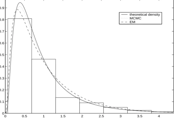
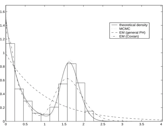
(14) following approximation,. ψ (u | η > 0, t, x) ≈. ³ ´ 1 X ψ u | λ(j) , k (j) , ω (j) , µ(j) , ν (j) . R (j) j:η. (25). >0. Finally, note that we can also obtain credible intervals for the estimated ruin probabilities (24) and (25). For example, the posterior median and 95% credible intervals can be obtained by just calculating the median and the 0.025 and 0.975 quantiles of the posterior sample {ψ(u | λ(j) , k (j) , ω (j) , µ(j) , ν (j) )}Jj=1 .. 5. Examples. In this section, we will illustrate the performance of the proposed methodology with various simulated risk processes covering a variety of features for the claim size distribution, such as multimodality or/and heavy tails, and considering different values for the safety loading. We will also compare our Bayesian approach with the classical MLE estimation based on the EM algorithm for PH distributions proposed in Asmussen et al. (1996). We initially consider a classical simple example based on 250 data generated from a lognormal distribution, LN (−0.32, 0.8). This example have been previously considered in the literature to model claim size data, see e.g. Asmussen & Roski (1991) and Bladt et al. (2003). Figure 1 illustrates a histogram of the data and the predictive density (12) estimated after running the MCMC algorithm for 10000 burn-in iterations followed by an additional 10000 iterations. This is compared with the classical density estimate based on the EM algorithm of Asmussen et al. (1996). The EM approach requires to fix previously the number of phases and then, we have chosen m = 4, as suggested in Asmussen & Roski (1991). With our Bayesian approach the posterior probability of the mixture size, k, is concentrated between 2 and 4 components. Conditional on k, the estimated values for νr , r = 1, ..., k, varies from 1 to 20. Thus, the predictive density is an average of densities with different number of phases that can be as small as 2 and as high as 140. FIGURE 1 ABOUT HERE Now, we consider a bimodal and platykurtic data set. We generate 300 data from a mixture of two Erlang components with parameters, k = 2, ω = (0.5, 0.5) , µ = (3, 0.6) and ν = (1, 50). The sample kurtosis is aproximately 1.32. Figure 2 shows the histogram of the data and the predictive density (12) obtained with the proposed MCMC algorithm. Our Bayesian method identifies the correct number of components in the mixture as the posterior mode of k is 2, with probability P (k = 2 | x) ' 0.72, which is obtained using (14). Much smaller posterior probabilities are obtained for k 6= 2. Also, conditional on k = 2, the parameters are. 14.

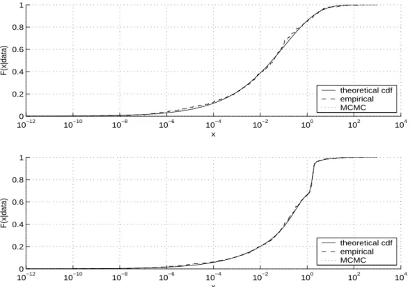
(15) estimated correctly, the posterior mean for ω, µ and ν are approximately given by (0.48, 0.52) , (3.32, 0.59) and (1, 53.4) , respectively. Figure 2 also compares the Bayesian estimation with two MLE density estimates obtained from the EM algorithm of Asmussen (1996) using a general PH and a Coxian distribution with 30 phases. Although we should have fixed the number of phases equal to 51, (note that the true generating Erlang mixture is a PH distribution with Σνr = 51 phases), the EM algorithm was numerically unfeasible with such a large number of phases. Observe that, using 30 phases, the first MLE density estimate, based on a general PH distribution, is statistically unstable and can not capture the bimodality of the distribution. The second MLE density estimate, based on a Coxian distribution, gives a better fit as the number of parameters to estimate is smaller. However in this case, the peaked shape of the second mixture component is not well approximated and a larger number of phases should be required for a better fit. Also, the MLE estimation requires a quite large computational cost of about 40 minutes. In contrast, our Bayesian density estimate, which is quite satisfactory, require a moderate computational cost of approximately 10 minutes. Finally, we have also observed that if the number of mixture components is increased, specially if they have relatively small variances, there are still more difficulties in obtaining good density estimates using the EM approach, while the MCMC algorithm is just slightly slowed in computational time but continues to be precise. FIGURE 2 ABOUT HERE Finally, we consider two long-tailed distributions. It is well known that although PH distributions are short-tailed, they can be used to approximate long-tailed distributions, see e.g. Feldmann & Whitt (1998) and Horvath & Telek (2000). We generate 300 data from a Weibull distribution, whose cdf is given by c. F (x) = exp {− (dx) }, and we set c = 0.3 and d such that the distribution mean is 1. This long-tailed distribution model have been previously considered in Feldmann & Whitt (1998) and Ausin et al. (2005). Additionally, in order to define a data set with both bimodal and long-tailed distribution, we also consider the 300 observations from the previous example plus these 300 Weibull data. Figure 3 illustrates in log scale the theoretical, empirical and predictive cumulative distribution functions obtained with (13) for both examples. Observe that the fits are quite satisfactory, even for the bimodal case. The number of mixture components required to approximate these data is quite large. In fact, the posterior modes of k are 7 and 8 for the unimodal and bimodal data sets, respectively. Unfortunately, we have not been able to compare the predictive densities with the MLE estimates because the EM algorithm of Asmussen (1996) was detained for these data sets, wether we consider a general PH or a Coxian distribution with more than four phases. However, we have compared these predictive distributions with those obtained using a Bayesian approach based on a Coxian distribution proposed in Ausin et al. (2005) and we have observed that the Coxian model can capture the heavy-tailed behaviour but, it can hardly approximate the bimodality. Also the number of 15.

(16) parameters and the computational cost required is much larger with the Coxian distribution than with the Erlang mixture model. FIGURE 3 ABOUT HERE Now, we can address the problem of ruin probability estimation. We consider four simulated risk processes using the four claim size data sets generated previously from a classical unimodal, a bimodal, a long-tailed and a long-tailed bimodal distributions. Note that the first classical example is also a long-tailed distribution as the lognormal distribution is long-tailed, but the tail of the considered lognormal LN (−0.32, 0.8) do not decay much more slowly than exponentially. Firstly, in order to examine the effects of “heavy traffic” in the data, we fix the safety loading η to be equal to 0.10, which implies that the average income of the insurance company is only 10% larger than the average loss per unit of time. Note that the true mean claim size in the four cases is equal to 1 and then, the value of the interarrival rate is given by λ = 0.9091, see (17) which, for simplicity, is assumed to be known. We also assume that the premium rate is c = 1. Table 1 shows the estimated posterior probabilities that the safety loading is positive, see (21), and their posterior means for the four risk processes, see (22). Observe that the posterior probability of having a stable process is very large for the classical and bimodal examples. However, we can observe in the last two cases that the long-tailed claims sizes together with a large interarrival rate have produced a small posterior probability of having a stable process. Also, note that the posterior means of the safety loading are close to the true value in the classical and the bimodal example, but in the two long-tailed examples, it is only well estimated when the risk process is assumed to be stable. TABLE 1 ABOUT HERE Figure 4 illustrates the estimated ruin probabilities as a function of the initial capital, u, for each of the four cases unconditioned and conditioned on η > 0, obtained from (24) and (25), respectively. As expected, ruin probabilities are smaller when the safety loading is imposed to be positive. These differences are stronger for the long-tailed cases. With or without this restriction, the estimated ruin probabilities are much smaller for the classical and bimodal examples than for the long-tailed distributions. This should be expected because the sample coefficients of variation in the classical and bimodal examples are given by 1.04 and 0.72, respectively, which indicates that the ruin probabilities will be close to those obtained with an exponential claim size distribution whose coefficient of variation is equal to 1. On the contrary, the sample coefficient of variation in the last two long-tailed cases are given by 8.62 and 7.59, respectively, and then, much larger ruin probabilities than for the exponential case should be expected. 16.

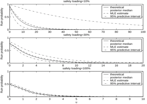
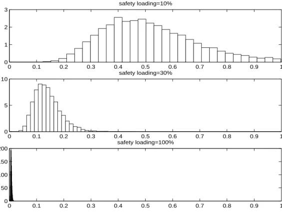
(17) FIGURE 4 ABOUT HERE Our Bayesian approach also allows for the calculation of predictive intervals for the estimated ruin probabilities, as commented in Section 4. Figure 5 illustrates the posterior medians and 95% predictive intervals of the ruin probabilities for the case with bimodal claim size distribution and different values of the safety loading. Note that the safety loadings are fixed to 10%, 30% and 100% which implies that the interarrival rates are fixed to 0.909, 0.769, and 0.5, respectively. Observe that the larger is the safety loading, the wider are the predictive intervals of the estimated ruin probabilities. Note also that the predictive intervals of the ruin probabilities are left-skewed, specially for larger safety loadings. Thus, the posterior medians of the ruin probabilities will be better estimates than the posterior means. In order to check the accuracy of the estimations, the posterior medians are compared with the theoretical ruin probabilities. Finally, the ruin probability estimates are also compared with those obtained with the EM approach. Note that both MLE estimates and theoretical ruin probabilities are similar to the Bayesian estimates and are always inside the predictive intervals. FIGURE 5 ABOUT HERE Finally, note that for each initial capital we have a whole predictive sample of ruin probabilities which has been used to calculate the corresponding 95% predictive interval. This posterior sample can also be used to compute any required quantile of the posterior distribution of each ruin probability. For example, given an initial capital of u = 6 units, Figure 6 shows the histograms of the posterior samples of ruin probabilities that have been obtained to calculate the predictive intervals in Figure 5 for u = 6. We can again observe the asymmetry of the predictive ruin probability distributions and that their variances decrease when the safety loading increases. FIGURE 6 ABOUT HERE. 6. Discussion and extensions. In this article, we have developed a Bayesian approach to make inference and prediction for the classical compound Poisson risk reserve process with unknown claim size distribution. Firstly, we have proposed a Bayesian density estimation method based on mixtures of Erlang distributions for the approximation of the general claim size distribution. We have illustrated that using a special reparameterization of the Erlang mixture model it is possible to approximate both long-tailed or/and multimodal claim size distributions. Using that the Erlang mixture model is a phase-type distribution, we have also described a Bayesian procedure for the estimation of ruin probabilities and other system quantities. The proposed Bayesian 17.

(18) approach provides confidence intervals for the estimated ruin probabilities and directly incorporates the uncertainty in the estimated safety loading without imposing the equilibrium condition. Our Bayesian approach could be extended to the more general Sparre Andersen risk model by considering Erlang mixtures for both the claim interarrival and claim size distributions. Explicit expressions for the ruin probabilities in this risk model can be derived using the phase-type properties of the Erlang mixture model, see Asmussen & Rolski (1991) and Asmussen (2000). Furthermore, extensions to more complicated situations with non-independent interarrival times, such as Markov modulated Poisson arrivals, should be possible using the Bayesian inference developed in Scott & Smyth (2003). Then, ruin probabilities in risk processes with Markov modulated Poisson arrivals and Erlang mixture claim sizes could be estimated using the results derived in Asmussen & Rolski (1991). Many other results from the risk theory related to phase-type distributions could be combined with our Bayesian procedure in order to estimate other quantities of interest. For example, given the observed data, we could estimate the deficit at ruin in the aforementioned Sparre Andersen model using the results obtained by Drekic et al. (2004) and Dickson & Drekic (2004). Another example is the Bayesian estimation of finite time ruin probabilities using the explicit expressions of their Laplace transform derived in Avram & Usabel (2003). In this case, the MCMC approach could be combined with numerical inversion methods of Laplace transforms in order to obtain point estimates and credible intervals for the finite time ruin probabilities. Finally, a further extension is the estimation of ruin probabilities in multivariate compound Poisson risk models that could be developed using the results given in Cai & Li (2005).. References ABRAMOWITZ, M., & STEGUN, I.A., (1964). Handbook of Mathematical Functions. New York: Dover. ARMERO, C., & BAYARRI, M.J., (1994). Bayesian prediction in M/M/1 queues. Queueing Syst., 15, 401-417. ARMERO, C., & CONESA, D., (2004). Statistical performance of a multiclass bulk production queueing system. Eur. J. Oper. Res., 158, 649-661. ASMUSSEN, S., (2000). Ruin probabilities. Advanced Series on Statistical Science & Applied Probability (Vol. 2). Singapore: World Scientific. ASMUSSEN, S., NERMAN, O., & OLSSON, M., (1996). Fitting phase-type distributions via the EM algorithm. Scand. J. Stat., 23, 419-441.. 18.

(19) ASMUSSEN, S., & ROLSKI, T., (1991). Computational methods in risk theory: A matrix-algorithmic approach. Insur. Math. Econ. 10, 259-274. AUSIN, M.C., LILLO, R.E., RUGGERI, F., & Wiper, M.P., (2003). Bayesian modelling of hospital bed occupancy times using a mixed generalized Erlang distribution. In Bayesian Statistics 7, eds. J. M. Bernardo, M. J. Bayarri, J. O. Berger, A. P. Dawid, D. Heckerman, A. F. M. Smith, M. West, pp. 443-452. Oxford: Oxford University Press. AUSIN, M.C., WIPER, M.P., & LILLO, R.E., (2004). Bayesian estimation for the M/G/1 queue using a phase type approximation. J. Stat. Plan. Infer., 118, 83-101. AUSIN, M.C., WIPER, M.P., & LILLO, R.E., (2005). Transient Bayesian inference for short and long-tailed GI/G/1 queueing systems. Working paper 05-36-05. Statistics and Econometrics Series. Universidad Carlos III de Madrid. AVRAM, F., & USABEL, M., (2003) Finite time ruin probabilities with one Laplace inversion. Insur. Math. Econ., 32, 371-377. BLADT, M., GONZALEZ, A., & LAURITZEN, S.L., (2003). The estimation of phase-type related functionals using Markov Chain Monte Carlo methods. Scand. Actuarial J., 2003, 280-300. CAI, J., & Li, H., (2005). Multivariate risk model of phase type. Insur. Math. Econ., 36, 137-152. CAIRNS, A.J.G., (2000). A discussion of parameter and model uncertainty in insurance. Insur. Math. Econ., 27, 313-330. DICKSON, D.C.M., & DREKIC, S., (2004). The joint distribution of the surplus prior to ruin and the deficit at ruin in some Sparre Andersen models. Insur. Math. Econ., 34, 97-107. DREKIC, S., DICKSON, D.C.M., STANFORD, D.A., & WILLMOT, G.E., (2004). On the distribution of the deficit at ruin when claims are phase-type. Scand. Actuarial J., 2, 105-120. DIEBOLT, J., & ROBERT, C.P. (1994). Estimation of finite mixture distributions through Bayesian sampling. J. Roy. Stat. Soc. B, 56, 363-375. FADDY, M.J., (1994). Examples of fitting structured phase-type distributions. Appl. Stoch. Model. Data Anal., 10, 247-255. FELDMANN, A., & WHITT, W. (1998). Fitting mixtures of exponentials to long-tail distributions to analyze network performance models. Perform. Evaluation, 31, 245-279 19.

(20) GREEN, P., (1995). Reversible jump MCMC computation and Bayesian model determination. Biometrika, 82, 711 732. GRUET, M. A., PHILIPPE, A., & ROBERT, C. P. (1999). MCMC control spreadsheets for exponential mixture estimation. J. Comput. Graph. Stat., 8, 298-317. HIPP, C., (1989). Estimates and boostrap confidence intervals for ruin probabilities. Astin Bull., 19, 57-70. HORVATH, A., & TELEK, M., (2000). Approximating heavy tailed behavior with phase-type distribution. In Advances in Algorithmic Methods for Stochastic Models, eds. G. Latouche, P. Taylor, pp. 191-214, Notable Publications. JOHNSON, M.A., & TAAFFE, M.R., (1991). An investigation of phase-distribution moment-matching algorithms for use in queueing models. Queueing Syst., 8, 129148. KEATINGE, C.L., (1999). Modeling losses with the mixed exponential distribution. Proceedings of the Casualty Actuarial Society, 1999, Volume LXXXVI, 165, 654-681. MOLER, C., & VAN LOAN, C., (1978). Nineteen dubious ways to compute the exponential of a matrix. SIAM Rev., 20, 801-836. NEUTS, M.F., (1981). Matrix Geometric Solutions in Stochastic Models. Baltimore: Johns Hopkins University Press. PHILIPPE, A. (1997). Simulation of right- and left-truncated gamma distribution by mixtures. Stat. Comput., 7, 173-182. RICHARDSON, S., & GREEN, P., (1997). On Bayesian analysis of mixtures with an unknown number of components. J. Roy. Stat. Soc. B, 59, 731 792. RIOS, D., WIPER, M.P., & RUGGERI, F., (1998). Bayesian analysis of M/Er/1 and M/Hk /1 queues, Queueing Syst., 30, 289-308. ROBERT, C.P., & MENGERSEN, K.L., (1999). Reparameterisation Issues in Mixture Modelling and their bearing on MCMC algorithms. Comput. Stat. Data Anal., 29, 325-343. ROLSKI, T., SCHMIDLI, H., SCHMIDT, V., TEUGELS, J., (2000). Stochastic processes for insurance and finance. New York: John Wiley & Sons. SCOTT, S.L., & Smyth, P., (2003). The Markov Modulated Poisson Process and Markov Poisson Cascade with applications to web traffic data. In Bayesian Statistics 7, eds. J.M. Bernardo, M.J. Bayarri, J.O. 20.

(21) Berger, A.P. Dawid, D. Heckerman, A.F.M. Smith, M. West, pp. 671-680. Oxford: Oxford University Press. SCHMICKLER, L., (1992). MEDA: mixed Erlang distributions as a Phase-type representations of empirical distribution functions. Stoch. Models, 8, 131-156. WIPER, M.P., (1998). Bayesian analysis of Er/M/1 and Er/M/c queues, J. Stat. Plan. Infer., 69, 65-79.. Appendix. Here, we show that the joint posterior distribution of the model parameters, θ = (k, ω, µ1 , τ , ν) , is proper given the improper joint prior distribution assumed in Section 3, see (6), (7), (8) and (9), and the likelihood corresponding to (4). Thus, we have to show that the following integral is finite, Z f (θ). n Q i=1. µ. k P. ¶ ωr Er (xi | νr , µr ) dθ.. r=1. Assume first that the number of observations is n = 1, then this integral is proportional to, Ã k ! ν f (k) f (ω|k) f (τ |k) f (ν|k) X (νr µ1 τ2 ...τr ) r νr −1 ωr x1 exp {−νr µ1 τ2 ...τr x1 } dθ µ1 Γ (νr ) r=1 Z X Z k ν ωr (νr τ2 ...τr x1 ) r νr −1 = f (k) f (ω|k) f (τ |k) f (ν|k) µ1 exp {−νr τ2 ...τr x1 µ1 } dθ x Γ (νr ) r=1 1 Z X Z Z X k k 1 ωr ωr = f (k) f (ω|k) f (τ |k) f (ν|k) dθ −µ1 = f (ω|k) f (k) dωdk = < ∞, x x x1 r=1 1 r=1 1. Z. where we have denoted θ −µ1 = (k, ω, τ , ν) . Observe that it is sufficient to have proved that the integral is finite for n = 1, because if n > 1, we can define f (θ | x1 ) as a new proper prior and consider the likelihood based on {x2 , ..., xn }, which is regular and proper, in which case the posterior is known to be proper. Now, we show that the posterior mean of the safety loading given in (22) is also finite. Using the independence assumption between the arrival and size of claims, "µ E [η | t, x] = E. k ω P r λ r=1 µr. ¶−1. Ã !−1  k X £ −1 ¤ ωr − 1 | t, x = E λ | t E  | x − 1, µ r=1 r #. which is finite because using (20), P £ −1 ¤ δ + m i=1 ti < ∞, E λ |t = γ+m−1. 21.

(22) Pk for γ > 1, and similarly as before, when n = 1, we have that E[( r=1 ωµrr )−1 | x1 ] is proportional to, Ã k ! ν f (k) f (ω|k) f (τ |k) f (ν|k) X (νr µ1 τ2 ...τr ) r νr −1 ωr x1 exp {−νr µ1 τ2 ...τr x1 } dθ Pk Γ (νr ) µ1 r=1 µ1 τω2r...τr r=1 ! Ã k Z ν 1 f (k) f (ω|k) f (τ |k) f (ν|k) X (νr τ2 ...τr x1 ) r νr = µ1 exp {−νr µ1 τ2 ...τr x1 } dθ ωr Pk ωr x1 Γ (νr ) r=1 r=1 τ2 ...τr Ã k ! Z 1 f (k) f (ω|k) f (τ |k) f (ν|k) X ωr = 2 dθ Pk ωr x1 ν τ ...τr r=1 r 2 r=1 τ2 ...τr Ã k ! Z 1 f (k) f (ω|k) f (τ |k) f (ν|k) X ωr 1 ≤ 2 dθ = 2 < ∞, Pk ω r x1 τ ...τr x1 r=1 2 r=1. Z. τ2 ...τr. Then, using the same arguments as above, this integral is also finite for n > 1.. 22.

(23) Figure 1: Histogram of the lognormal data set with the theoretical, Bayesian and maximum-likelihood density estimates. Figure 2: Histogram of the two component mixture data set with the theoretical and Bayesian predictive densities compared with two maximum-likelihood density estimates based on a general PH and a Coxian distribution with 30 phases. Figure 3: Theoretical, empirical and predictive cumulative distribution functions for the long-tailed Weibull data set (top) and for the mixture of long-tailed and bimodal data set (botton). Figure 4: Predictive ruin probabilities as function of the initial capital for each of the four simulated risk processes unconditioned (left) and conditioned (right) on η > 0. Figure 5: Posterior medians of the ruin probabilities and 95% predictive intervals as a function of the initial capital for the bimodal claim size data and different values of the safety loading compared with the EM estimates and theoretical values. Figure 6: Histogram of the predictive samples of ruin probabilities for the bimodal claim size data and different values of the safety given an initial capital of u = 6 units.. 23.

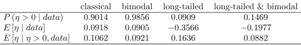
(24) Table 1: Posterior probabilitities that the safety loading, η, is positive and their posterior means unconditioned and conditioned on η > 0 for the four simulated risk proccesses. P (η > 0 | data) E [η | data] E [η | η > 0, data]. classical 0.9014 0.0918 0.1062. bimodal 0.9856 0.0905 0.0921. 24. long-tailed 0.0909 −0.3566 0.1636. long-tailed & bimodal 0.1469 −0.1977 0.0882.

(25) 0.9 theoretical density MCMC EM. 0.8. 0.7. 0.6. 0.5. 0.4. 0.3. 0.2. 0.1. 0. 0. 0.5. 1. 1.5. 2. 2.5. 3. 3.5. 4. Figure 1: Histogram of the lognormal data set with the theoretical, Bayesian and maximum-likelihood density estimates.. 25.

(26) 1.6. theoretical density MCMC EM (general PH) EM (Coxian). 1.4. 1.2. 1. 0.8. 0.6. 0.4. 0.2. 0. 0. 0.5. 1. 1.5. 2. 2.5. 3. 3.5. 4. Figure 2: Histogram of the two component mixture data set with the theoretical and Bayesian predictive densities compared with two maximum-likelihood density estimates based on a general PH and a Coxian distribution with 30 phases.. 26.

(27) 1. F(x|data). 0.8 0.6 0.4 theoretical cdf empirical MCMC. 0.2 0 −12 10. −10. −8. 10. −6. 10. −4. 10. −2. 10 x. 0. 10. 2. 10. 4. 10. 10. 1. F(x|data). 0.8 0.6 0.4 theoretical cdf empirical MCMC. 0.2 0 −12 10. −10. −8. 10. −6. 10. −4. 10. −2. 10 x. 0. 10. 2. 10. 4. 10. 10. Figure 3: Theoretical, empirical and predictive cumulative distribution functions for the long-tailed Weibull data set (top) and for the mixture of long-tailed and bimodal data set (botton).. 1. 1. 0.9. 0.9. 0.8. 0.8. 0.7. 0.7 classical bimodal long−tailed long−tailed & bimodal. 0.6 psi(u|data). psi(u|data). 0.6. 0.5. 0.5. 0.4. 0.4. 0.3. 0.3. 0.2. 0.2. 0.1. 0.1. 0. classical bimodal long−tailed long−tailed & bimodal. 0. 10. 20. 30. 40. 50 u. 60. 70. 80. 90. 100. 0. 0. 10. 20. 30. 40. 50 u. 60. 70. 80. 90. 100. Figure 4: Predictive ruin probabilities as function of the initial capital for each of the four simulated risk processes unconditioned (left) and conditioned (right) on η > 0.. 27.

(28) safety loading=10%. Ruin probability. 1 theoretical posterior median MLE estimate 95% predictive interval. 0.5. 0. 0. 10. 20. 30. 40 50 60 safety loading=30%. 70. 80. 90. 100. Ruin probability. 1 theoretical posterior median MLE estimate 95% predictive interval. 0.5. 0. 0. 2. 4. 6. 8 10 12 safety loading=100%. 14. 16. 18. 20. Ruin probability. 1 theoretical posterior median MLE estimate 95% predictive interval. 0.5. 0. 0. 1. 2. 3. 4. 5 u. 6. 7. 8. 9. 10. Figure 5: Posterior medians of the ruin probabilities and 95% predictive intervals as a function of the initial capital for the bimodal claim size data and different values of the safety loading compared with the EM estimates and theoretical values.. 28.

(29) safety loading=10% 3 2 1 0. 0. 0.1. 0.2. 0.3. 0.4 0.5 0.6 safety loading=30%. 0.7. 0.8. 0.9. 1. 0. 0.1. 0.2. 0.3. 0.4 0.5 0.6 safety loading=100%. 0.7. 0.8. 0.9. 1. 0. 0.1. 0.2. 0.3. 0.4. 0.7. 0.8. 0.9. 1. 10. 5. 0 200 150 100 50 0. 0.5. 0.6. Figure 6: Histogram of the predictive samples of ruin probabilities for the bimodal claim size data and different values of the safety given an initial capital of u = 6 units.. 29.

(30)