Operating cost risk analysis for an underground mining project

Texto completo

(1)PONTIFICIA UNIVERSIDAD CATOLICA DE CHILE ESCUELA DE INGENIERIA. OPERATING COST RISK ANALYSIS FOR AN UNDERGROUND MINING PROJECT. VICENTE MOBAREC KATUNARIC. Thesis submitted to the Office of Research and Graduate Studies in partial fulfillment of the requirements for the Degree of Master of Science in Engineering. Advisor: ÁLVARO VIDELA LEIVA. Santiago de Chile, January, 2015  2015, Vicente Mobarec Katunaric.

(2) PONTIFICIA UNIVERSIDAD CATOLICA DE CHILE ESCUELA DE INGENIERIA. OPERATING COST RISK ANALYSIS FOR AN UNDERGROUND MINING PROJECT. VICENTE JOSÉ MOBAREC KATUNARIC. Members of the Committee: ÁLVARO VIDELA LEIVA JOSÉ BOTÍN GONZÁLEZ EDISSON PIZARRO CARVAJAL JORGE GIRONÁS LEÓN. Thesis submitted to the Office of Research and Graduate Studies in partial fulfillment of the requirements for the Degree of Master of Science in Engineering Santiago de Chile, January, 2015.

(3) To my parents, for their unconditional support and guidance.. ii.

(4) ACKNOWLEDGMENTS I would like to express my gratitude to my supervisor Dr. Alvaro Videla for the useful comments, remarks and engagement through the learning process of this master thesis. Thank for your trust and guidance. I would also like to express my appreciation to CODELCO and the Department of Mining Engineer of Pontificia Universidad Católica. Thanks for giving the opportunity to be part of the Codelco-PUC investigation group. Special thanks to Edisson Pizarro for his time and assistance. Finally, i would like to thank my loved ones, for their support and encouragement not only during this process, but throughout my life. I will be grateful forever for your love.. iii.

(5) TABLE OF CONTENTS. ACKNOWLEDGMENTS ............................................................................................... iii TABLE OF CONTENTS ..................................................................................................iv LIST OF TABLES ............................................................................................................vi LIST OF FIGURES ........................................................................................................ vii ABSTRACT ................................................................................................................... viii RESUMEN........................................................................................................................ix 1.. INTRODUCTION ...................................................................................................... 1 1.1. 2.. Problem Description ............................................................................................. 3. OBJECTIVES & METHODOLOGY ......................................................................... 4. 3. CASE STUDY - CHUQUICAMATA UNDERGROUND MINE PROJECT ........... 5 3.1. Context .................................................................................................................. 5. 3.2. Input Data .............................................................................................................. 6. 3.3. Pareto Analyis ....................................................................................................... 8. 3.4. Identification and Categorization of Cost Generators ........................................... 9. 3.5. Cost Generators Modelling ................................................................................... 9 3.5.1 Input Prices .............................................................................................. 10 3.5.2 Consumption Intensities .......................................................................... 11 3.5.3 Production & Development Requirements .............................................. 13. 4.. SIMULATION .......................................................................................................... 14 4.1. Results ................................................................................................................. 14. 4.2. Risk Assessment & Quantification ..................................................................... 15. iv.

(6) 4.3. Risk Managment ................................................................................................. 17 4.3.1 Energy...................................................................................................... 18 4.3.2 Labor........................................................................................................ 22. 5.. CONCLUSIONS ....................................................................................................... 25. REFERENCES................................................................................................................. 27 APPENDIX ...................................................................................................................... 30 A. Cost Sub-activities .................................................................................................. 31 B. Pareto Analysis ........................................................................................................ 34 C. Input Prices: Data Series ......................................................................................... 35 D. Input Prices: Calculated Standard Deviations and Correlations ............................. 36 E. Consumption Intensities: Correlations and Autocorrelations .................................. 38 F. Production Energy Consumption Models (MB-N1) ................................................ 40 G. Production & Development Requirements ............................................................. 45 H. Simulation Inputs Table .......................................................................................... 46. v.

(7) LIST OF TABLES. Table I: CUMP Operational Cost Structure ....................................................................... 7 Table II: Initial Input Prices and Standard Deviations for 2015, 2020, 2025 and 2030. . 11 Table III: Modeled Distributions and CVs for the Elements of Expenditure of CUMP.. 12 Table IV: Energy Cost Items Economic Risk in Present Value ...................................... 16 Table V: Labour Cost Items Economic Risk in Present Value ........................................ 17 Table VI: Solar PV Plant Average Cost & Parameters .................................................... 19 Table VII: Cost Items Identified in the Pareto Analysis .................................................. 34 Table VIII: Historic Data Series for the Input Prices ....................................................... 35 Table IX: Standard Deviations for the Input Prices ......................................................... 36 Table X: Correlation Matrix for th Input Prices............................................................... 37 Table XI: Correlation Matrix for the Development Consumption Intensities ................. 38 Table XII: Correlation Matrix for the Production Consumption Intensities .................... 38 Table XIII: Autocorrelation Results for the Development Consumption Intensities ...... 39 Table XIV: Autocorrelation Results for the Production Consumption Intensities .......... 39 Table XV: CECI Comparison between the Regression Model and CUMP Feasibility... 41 Table XVI: CUMP CECI Modeled Distribution ............................................................. 43 Table XVII: VECI Comparison between the Regression Model and CUMP Feasibility 43 Table XVIII: CUMP VECI Modeled Distribution .......................................................... 44 Table XIX: CUMP Production & Development Plan ...................................................... 45 Table XX: Input Prices Models........................................................................................ 46 Table XXI: Consumption Intensities Models .................................................................. 46. vi.

(8) LIST OF FIGURES. Figure 1: Proposed Methodology for the Operating Cost Risk Analysis. ......................... 5 Figure 2: Schematic Diagram of CUMP Operation ........................................................... 6 Figure 3: Contribution of the Elements of Expenditure to the Operating Costs ................ 9 Figure 4: CUMP Operational Cost Net Present Value Probability Distribution ............. 14 Figure 5: Contribution of Elements of Expenditure to the Calculated Economic Risk. .. 15 Figure 6: CUMP Operational Cost + Solar Plant Probability Distribution..................... 20 Figure 7: CUMP Operational Cost + Labor Price Growth Probability Distribution. ..... 23 Figure 8: CECI vs Elevation Regression Model .............................................................. 40 Figure 9: CECI Prediction Interval and Regression Model ............................................. 42. vii.

(9) ABSTRACT. Traditional risk quantification methods currently used for estimating operating costs of mining projects provide little information as to the sources of risk. Rather, they tend to produce static and over-conservative evaluations, which do not account for changes in market conditions or project performance indicators. Decisions relating to the operating costs of large mining projects require more sophisticated risk evaluation models. These must be capable of quantifying the growing range of uncertainty, integrating alternative scenarios and strategies into the evaluation, thereby helping the management decisionmaking process. In this study we present a systematic model for managing the economic risk of the operating costs for an ongoing mining project. Firstly, we identify the key cost generators of the project and characterize their inherent variability. Secondly, using Monte Carlo simulation, we incorporate this variability into the evaluation and quantify the economic risk. Finally, we identify the main risk sources, for which we propose risk mitigation actions. The model is validated by means of a case study into the new Chuquicamata Underground Mine Project. The results show that the variability of the cost generators can potentially increase the present value of the estimated operating cost of the project by more than 10%, with labor and energy being the most relevant risk sources. Some of the proposed risk mitigation alternatives that are currently being considered by the project managers include the construction of a solar power plant for the operation and the implementation of specific labor productivity improvement strategies.. Keywords: Risk Quantification, Risk Management, Underground Mining Operating Cost, Monte Carlo simulation, Quantitative Risk Analysis.. viii.

(10) RESUMEN. Los métodos tradicionales que actualmente se utilizan para la cuantificación del riesgo asociado a los costos de operación de los proyectos mineros proporcionan poca información respecto de las fuentes y efectos del riesgo. Por el contrario, tienden a generar estimaciones estáticas y conservadoras, que no consideran los efectos que los posibles cambios en las condiciones del mercado o en los indicadores de desempeño generarían en el proyecto. Las decisiones asociadas a los costos de operación de grandes proyectos mineros requieren modelos más sofisticados de evaluación del riesgo. Estos deben ser capaces de identificar y cuantificar las incertidumbres, e integrar diferentes escenarios y estrategias en la evaluación, ayudando así al proceso de toma de decisiones. En esta investigación, se presenta un modelo integral para la gestión del riesgo económico de los costos de operación de un proyecto minero en desarrollo. En primer lugar, se identifican los principales generadores de costos del proyecto y se caracterizan sus variabilidades intrínsecas. En segundo lugar, mediante una simulación de Monte Carlo, se incorporan estas variabilidades a la evaluación y se cuantifica el riesgo económico. Por último, se identifican las principales fuentes de riesgo y se proponen medidas de mitigación para estas. El modelo es validado mediante un caso de estudio en el Proyecto Mina Chuquicamata Subterráneo. Los resultados muestran que la variabilidad de los generadores de costo puede aumentar el valor presente de los costos operativos estimados para el proyecto en más de un 10%, siendo la mano de obra y la energía las fuentes de riesgo más relevantes. Algunas de las medidas de mitigación de riesgos propuestas en este caso incluyen la construcción de una planta de generación eléctrica para abastecer al proyecto y la incorporación de nuevas estrategias de recursos humanos enfocadas en mejorar productividad de la mano de obra.. ix.

(11) 1. 1.. INTRODUCTION. The process of developing a large scale underground mining operation, from the primary discovery of an ore body to the actual extraction of minerals, takes several years and consists of different stages. These are generally defined as follows: Scoping, Prefeasibility, Feasibility, Engineering Design and Site Construction & Mine Development (Society for Mining, Metallurgy, and Exploration, 2011). Each stage consists of more detailed information than the preceding one, therefore reducing the levels of uncertainty (Tulcanaza, 2014). Based on this information, the key variables of the project are estimated. This enables a global economic evaluation to be developed for the future mining operation. In general terms, any economic evaluation of a mining project is defined by its projected financial results. The income of a mining operation is the product of the amount of metal produced and the selling price of that metal. Assuming the project has been correctly designed and achieves the expected production levels and recoveries, income may be considered an exogenous variable, depending on the price of the commodity being produced. On the other hand, the overall cost of a mining operation includes the addition of capital and operating costs. Capital costs refer to the investment required for the design and implementation of the mining operation, which takes place primarily during the early years of the project. In turn, operating costs relate to the expenses associated with all the unitary processes that make the mineral production possible, from the ore body characterization, to the extraction of the ore itself and its subsequent processing throughout the life of the mine (LOM). These operating costs will depend on both intrinsic and extrinsic variables. The former relate to the particular circumstances and requirements of the operation, and the latter to market conditions and commodity prices. Currently, and especially in recent years, operating costs in the Chilean mining industry have become a critical issue due to their substantial rise as a percentage of total spending (Perez-Oportus, 2008). At first glance, this upward trend does not indicate signs of.

(12) 2. stabilization. As a consequence, uncertainty and possible risks related to their variations during the LOM should be considered an important factor and included as part of any mining project evaluation, especially for projects in early stages of development. Since most large scale mining projects consider an LOM of at least a few decades, operating cost estimations and decisions cannot rely merely on static parametric evaluations such as discounted cash flow (DCF). This is because such methods provide only a snapshot of the value of a project associated to a ‘base case’ scenario, and fail to consider the dynamic character of decision-making over the life of the project (Botín, Del Castillo & Guzmán, 2013). Risk analysis techniques based on Monte Carlo simulation, such as Quantitative Risk Analysis (QRA), represent a more appropriate path to understanding the responses and robustness of a project. This is especially the case given the time frame and the intrinsic uncertainty associated with the estimation variables (Heuberger, 2005; Chinbat & Takakuwa, 2009; Brown, 2012). Unlike traditional methods that incorporate uncertainty as a percentage of the total expenditure, using factors such as “contingency” or “overall expenses”, QRA relies on stochastic modeling and simulation of the key project variables, and its use is common across many industries. However, in the mining industry we often work with sparse amounts of data, where the lack of applicable information and the inherent differences in operations between mine sites makes the risk quantification process and its universal application difficult. The need to understand the causes and sources of risk in this environment strongly suggest the need for a subjective analysis in conjunction with quantitative methods. This will allow the company to quantify increasing levels of uncertainty and help it to understand potential project responses to the range of possible variations in the future conditions. (Summers, 2008). Our proposed method includes a systematic risk management approach, combining both quantitative and qualitative analysis, in order to identify the main sources of risk and propose risk mitigation alternatives. This method can be applied to any mining project and is validated on the ongoing Chuquicamata Underground Mine Project. The results.

(13) 3. show that the operating economic risk of the project is heavily related to just a few of its cost generators. Risk can be managed by introducing specific risk mitigation alternatives that target these generators, thus reducing the levels of uncertainty and even improving the economic value of the project. The rest of this document is organized as follows. Firstly, we introduce the problem and objectives. We then present a case study based on our experience at Chuquicamata Underground Mine Project, followed by a discussion of the methodology and results. Some final remarks are then offered, suggesting how results can be incorporated into the ongoing project. The appendices contain details and specific values of the input parameters used in the case study. 1.1. Problem Description. The main problem is that economic evaluations, especially during early stages of a mining project, do not consider the inherent variability of the costs, nor identify the major risk factors associated therein. This usually leads to higher operating costs and lower performance indicators than expected (McCarthy, 2013; MacKenzie & Cusworth, 2007). In fact, according to Merrow (2011), almost 70% of mining megaprojects fail to meet at least one of their estimated key success criteria. By establishing a prompt and accurate characterization of the main risk sources, which impacts on the operating costs of the project, we are able to identify the critical risk factors, from among hundreds of items and activities. As a result, we can propose risk mitigation measures prior to the operation being commissioned. These measures aim to increase the overall value of the project and reduce the uncertainty of budget projections and result commitments. They may also include specific strategic investments or modifications of the technical and economic requirements initially considered..

(14) 4. 2.. OBJECTIVES & METHODOLOGY. The main objective of this study is to develop a model that can accurately identify the risk sources and quantify the economic risks of an underground mining project. The first major goal is to identify the main categories influencing the operating costs of the project and their cost generators, in order to focus our efforts on the most relevant variables. The second major goal is to study and characterize the variability of these cost generators and to include this variability in the evaluation process. To do this, the variables will be classified and modeled according to their nature. We will use market data to model the extrinsic variables, such as the price of the inputs, as well as information collected from other mining operations to model the intrinsic variables, such as the consumption intensities of the different inputs. By including the calculated variability as part of the project evaluation, the economic value of the uncertainty or economic risk can be quantified. This will enable us to identify the different risk elements and to rank them according to the economic impact they have on the project value. Finally, the last major goal is to propose and evaluate specific risk mitigation alternatives that target the most relevant risk sources and may include strategic investments or modifications of the technical and economic requirements initially considered. Figure 1 summarizes the proposed methodology..

(15) 5. Figure 1: The proposed methodology for the operating cost risk analysis consist of four steps. Firstly, we identify the main cost activities and their cost generators. Secondly, we model these cost generators as independent variables and include them into a simulation model. The simulation outputs will allow us to identify and rank the main risk elements according to their contribution to the total economic risk. Finally we quantify the risk associated with each risk element and propose risk mitigation alternatives for them.. 3.. CASE STUDY – CHUQUICAMATA UNDERGROUND MINE PROJECT. 3.1. Context. The Chuquicamata copper mine in Chile, owned by Codelco, has been operating as an open pit since 1915. Plans are currently being drawn up to go underground, as a fourpanel macro-block caving operation. The Chuquicamata Underground Mine Project (CUMP) is based on a production extraction rate of 140 kt/d, over a life span of 40 years, with a 7-year ramp-up, a 5-year ramp-down, and 28 years of steady production, plus almost 10 years of initial development. This will make it one of the largest underground operations in the world. The project is now beginning the detailed engineering stage, with production expected to start in 2019. Figure 2 shows a basic schematic diagram of the mine operation..

(16) 6. Figure 2: This figure shows an schematic diagram of CUMP operational activities.. 3.2. Input Data. Our CUMP case study includes all operating cost estimations as defined in the feasibility stage of the project. The data under investigation includes the development and production schedules, and all technical and economic parameters considered for the economic evaluation throughout the LOM (2019-2058). The present value of all operating costs of the project comes to US$2.582 billion (2014 US$, 8% discount rate), divided into two main activities: Development and Production costs. Each activity contains multiple sub-activities, which are then divided into elements of expenditure. The development costs include all the expenses related to the process of constructing the mining facility and the infrastructure to support it. The current estimation for the present value of the cost of this activity reaches US$844 million, which represents 30% of the total operating cost of the project. Development costs consist of ten sub-activities and seven elements of expenditure, with a total of 67 cost items. On the other hand, production costs include the expenses of all unitary operations involved in the actual.

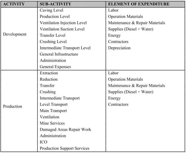
(17) 7. extraction of the ore from the ore body, including additional activities or services required to fulfill the mine production schedule. The current estimation for the present value of the cost of this activity is $1.738 billion, which represents the remaining 70% of the total operating costs. Production costs consist of 13 sub-activities and six elements of expenditure, with a total of 84 cost items. Table I summarizes the structure of the CUMP operating costs. The development and production sub-activities considered in this case study are explained in Appendix A. Table I: The table shows the operational cost structure of CUMP. There are two main activities: Development and Production. Each activity contains multiple sub-activities, which are then divided into elements of expenditure, generating a total of 151 cost items.. ACTIVITY. Development. Production. SUB-ACTIVITY Caving Level Production Level Ventilation Injection Level Ventilation Suction Level Transfer Level Crushing Level Intermediate Transport Level General Infrastructure Administration General Expenses Extraction Reduction Transfer Crushing Intermediate Transport Level Transport Main Transport Ventilation Mine Services Damaged Areas Repair Work Administration ICO Production Support Services. ELEMENT OF EXPENDITURE Labor Operation Materials Maintenance & Repair Materials Supplies (Diesel + Water) Energy Contractors Depreciation. Labor Operation Materials Maintenance & Repair Materials Supplies (Diesel + Water) Energy Contractors.

(18) 8. 3.3. Pareto Analysis. The first step is to identify the most relevant cost items of the total operating costs. As explained in the previous section, there are 151 cost items (67 from Development, plus 84 from Production) categorized in the following way: Activity – Sub-activity – Element of Expenditure. For the evaluation, we compared the different cost items according to their net present value of costs (NPVC). Considering the horizon of the project (40+ years), this alternative outweighs other available options, for example by comparing the items according to their added nominal value. This is because the use of a discount factor allows us to include the effect of time as part of the expenditure evaluation, resulting in a more realistic comparison. The NPVC of a cost item is calculated by adding up all the discounted expenses of that item throughout the LOM:. ,. 1. (1). This study uses 2014 as the initial year for the evaluation and an annual discount rate of = 8%, as defined by Codelco for this project. The total net present value of the operating costs of the project is calculated by adding up the NPVC of all cost items. For determining the most relevant cost items, we have used the Pareto principle, ranking and segregating those items that, in conjunction, represent 80% of the total operating cost net present value. From the analysis, we concluded that 30 out of 151 cost items (i.e. 19.86%) accounted for 80.2% of total expenditure. Of these 30 cost items, eight relate to development activities with an NPVC of US$678 million, and the other 22 to production activities, with a NPVC of US$1.394 billion. Figure 3 demonstrates the global proportion represented by each element of expenditure within these 30 cost items. Detailed information for these cost item is contained in Appendix B..

(19) 9. 7%. Labor. 10%. Energy. 34%. Operation Materials. 14%. Maintenance & Repair Materials Contractors. 15%. Others. 20%. Figure 3: This pie chart represents the contribution of each of the elements of expenditure identified by the Pareto analysis to the net present value of the operating costs.. 3.4. Identification & Categorization of Cost Generators. The relevant cost items identified in the previous section are analyzed in depth in order to isolate their specific cost generators. These cost generators are divided into three categories: Input Prices ( Development Requirements (. ), Consumptions Intensities ( ). The total expense (. ) and Production &. ) of each cost item identified. in the previous section, during any period of the evaluation, can be written as follows: $. 3.5. $. ∗. ∨. 2. ∗. ∨. 2. (2). Cost Generators Modeling. Having identified the main cost generators of the operating costs, we proceed to model their behavior by studying and characterizing their variability. The methodology for gauging the variability for elements of each cost category is explained as follows:.

(20) 10. 3.5.1 Input Prices The Input Prices represent the price per unit of the consumption of the inputs of each cost item. The inputs included as part of the CUMP case study (and which represent the main inputs of almost any underground mining project) are: energy, steel, concrete, diesel, explosives and labor. The unitary prices were modeled by combining the initial prices used in the feasibility stage of the project, plus their historical variability. This enabled us to obtain probability distribution functions that represent the possible behavior of the input prices through the LOM. By taking the historic prices of the observed inputs,. …. we define its price semi-variogram as follows: 1 2|. Where that. represents time in years, , and |. |. (3) ,. denotes the set of pairs of observations. ,. so. | is the number of pairs in the set. As defined by Isaaks &. Srivastava (1989), for every. , we can calculate the standard deviation as: (4). For generating forecasts, we model the input prices as random variables and assume they follow a normal distribution. ,. ; where. is the reference price estimation and. is the standard deviation defined above. This technique allows the model to gauge growing uncertainty over time relating to price forecasts, since. will increase when. increases. To estimate the standard deviations, we analyzed the real annual prices of the inputs over the last 20 years (1993-2013), as shown in Appendix C. The estimated standard deviations for the input prices are assumed to remain constant from 2030 onwards. Table II shows the reference price estimation and the standard deviation for each of the inputs for the years 2015, 2020, 2025 and 2030..

(21) 11. Table II: The table shows the reference prices for the inputs considered in the case study and their calculated standard deviations for 2015, 2020, 2025 and 2030. The standard deviation for all prices tend to increase when we move along the LOM, representing the growing uncertainty over time of the price forecasts. Input. Energy. Steel. Concrete. Diesel. Explosives. Labour. Po SD SD SD SD. US$/Mwh 100 7.0 21.8 26.5 27.0. US$/dmtu 142.1 13.6 28.2 41.4 50.8. Index 110 2.7 4.0 4.6 5.4. US$/liter 0.60 0.04 0.10 0.18 0.23. Index 110 2.6 3.8 4.4 6.2. Index 126 1.4 6.6 11.4 18.0. The considered price data series were then submitted to a correlation analysis. The results show a strong association among some of the input prices. We include this effect through a correlation matrix that will connect the modeled price distributions for each year of the evaluation. The calculated standard deviation of the input prices for the 20152030 period and their correlation matrix are contained and explained in appendix D. 3.5.2 Consumption Intensities Consider the consumption of inputs per unit of square meter developed or ton produced, depending on the activity in question. Consumption intensities will be related to the elements of expenditure of each activity, in this case: Labor, Materials, Supplies, Energy and Contractors. To estimate the consumption intensity generators, we have gathered official operational data from El Teniente Mine (Codelco), the only underground operation in Chile comparable in size to CUMP. This information was then paired with the base case estimations of the project. The collected data was arranged to match the cost structure of CUMP, taking into account the specific characteristics of the activities and elements of expenditure under investigation. Each series was analyzed using @Risk BestFit tool, as a means of establishing the distribution that most accurately reflected the data. Consumption intensities are now modeled as random variables that follow these distributions. Mean and spread parameters for the new distributions were determined by.

(22) 12. measuring the base case estimations and the collected data respectively. To evaluate the inherent variability of each of the consumption intensities under investigation, we calculate its coefficient of variation (CV), defined as the ratio of the standard deviation to the mean. We assume that even if the mean cost values between Teniente and CUMP consumptions differ, their CVs will be the same. In this way, we can estimate the standard deviation for the consumption intensities of CUMP in term of their initial estimated value. and its pairing with the CV of the El Teniente data series. as:. ∗. ∗. (5). The determined distributions and CVs for the activities and elements of expenditure evaluated in the case study are shown in Table III. Table III: The table shows the resulting distributions and CVs for the elements of expenditure considered in the case study. We model the consumption intensities as independent variables that follow these distributions, and calculate the distributions parameters using CUMP base case estimations and the presented CVs. ACTIVITY Development Development Development Development Production Production Production Production Production. ELEMENT OF EXPENDITURE Labor Operation Materials Energy Contractors Labor Operation Materials Maintenance & Repair Materials Supplies (Diesel + Water) Contractors. DISTRIBUTION Uniform Triangular Uniform Normal Laplace Normal Triangular Triangular Uniform. CV 27.20% 35.27% 25.71% 29.25% 12.97% 39.10% 13.63% 17.84% 27.53%. The considered consumption intensities of each activity’s elements of expenditure were submitted to a correlation analysis, and again a strong association between some of them was found. Autocorrelation tests were also performed for the data series, but no.

(23) 13. significant autocorrelations were found. The resulting matrices for the correlation and autocorrelation analyses are shown in Appendix E. The energy consumption intensities of the production cost items, associated with transport and ventilation sub-activities, were modeled using a different approach. Firstly, energy consumption non-linear regression models were developed using information from different mining operations. The models were then linearized and 95% confidence intervals were established. Finally, the energy consumptions for each of the subactivities were modeled. The modeling assumed their normal behaviour with a mean defined by the base case estimations. It also assumed a standard deviation associated with the spam between the maximum and minimum value of the confidence intervals estimated using the regression models. This alternative yet more exhaustive method was preferred, since there was a lack of data available in El Teniente mine for generating an accurate model for these specific consumption intensities. The full methodology is explained in Appendix F. For the case study, the depreciation consumption intensity is not modeled. This is because it primarily depends on capital investment decisions and national and organizational depreciation policies, rather than being directly related to the operating variables of the project. 3.5.3 Production & Development Requirements Represent the amount of square meters that will be developed and the number of tons that will be produced in each period of the LOM. The preliminary Production & Development plan for CUMP over the life of the project has been approved by Codelco and will be considered a fixed input for this research. The details of the plan are outlined in Appendix G..

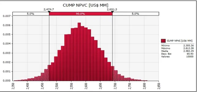
(24) 14. 4.. SIMULATION. The simulation was carried out using the @ Risk (Palisade) software with N=10000 iterations. We evaluated as input data the operational cost structure proposed in the project feasibility study, as well as the models and correlation matrices defined in the Cost Generators Modeling section. A detailed simulation input table is outlined in Appendix H. The main output of the simulation will be a distribution function of the net present value of the operating costs of the project. The probability distribution function obtained is shown in Figure 4.. Figure 4: This figure shows the probability distribution functions for the net present value of CUMP operating costs. The results illustrate the effect of including the variability of the cost generators into the evaluation, providing a more “realistic” cost estimation for the project.. 4.1. Results. The simulated NPV of the operational costs of the project range from US$2.351 to US$2.829 billion, with a mean of US$2.582 billion and a standard deviation of US$65.9 million. The mean value matches the value estimated for the base case scenario, as we.

(25) 15. determined the base case estimations as the mean values of the input variables. In doing so, we can isolate the effects of the variabilities of the cost generator in order to identify the major risk sources. 4.2. Risk Assessment & Quantification. To identify the major risk sources of the project, we define “Unacceptable” scenarios and calculate the economic risk as the difference between their mean value and the base estimation. Subsequently, we rank the elements of expenditure according to their contribution to the total economic risk posed. For the CUMP case study, we assume that the top 5% of simulated scenarios, i.e. the scenarios in which the present value of the operational cost exceeds the US$2.692 billion, are unacceptable. The mean present value of these scenarios is US$2.72 billion, generating a total economic risk of US$138 million. The average contribution of each element of expenditure to the calculated economic risk is shown as a Pie Chart in Figure 5.. 2% 6%. 5%. Labor. 31% 17%. Energy Operation Materials Maintenance & Repair Materials Contractors. 39%. Supplies. Figure 5: This pie chart shows the contribution of the elements of expenditure to the calculated economic risk value. We see that Labor and Energy account for 70% of the risk, which makes them our main risk elements.. As we can see from Figure 5, the most relevant risk sources are Energy and Labor, which together account for 70% of the total simulated risk. The risk mitigation efforts.

(26) 16. should focus on these elements of expenditure. Also, by contrasting these results with Figure 3, we conclude that economic risk is not always proportional to total expenditure. This validates the necessity for each of the elements of expenditure to be analyzed independently. Now we need to understand how this risk is distributed among the labor and energy related cost items. Using the same set of “unacceptable” scenarios, we quantify the specific economic risk of these cost items as the difference between their mean present value under these scenarios and their base case estimation. The resulting economic risk for the energy and labor cost items is shown in Tables 4 and 5 respectively. Table IV: This table shows the present value of the economic risk calculated for the four energyrelated sub activities. We see that the risk is heavily associated with the Main Transport and Ventilation sub activities. Activity Development Production Production Production TOTAL. Sub-Activity Production Level Level Transport Main Transport Ventilation. Element of Expenditure Energy Energy Energy Energy. RPV $MM 5.1 3.7 28.2 16.4 53.4.

(27) 17. Table V: This table shows the present value of the economic risk calculated for the labor-related sub activities. In this case, there are eleven sub-activities and the risk is more evenly distributed among them. Activity Development Development Production Production Production Production Production Production Production Production Production. Sub-Activity Caving Level Production Level Extraction Reduction Transfer Crushing Intermediate Transport Mine Services Damaged Areas Repair Work Administration ICO. TOTAL. Element of Expenditure Labor Labor Labor Labor Labor Labor Labor Labor Labor Labor Labor. RPV $MM 7.3 6.2 4.9 4.2 3.3 2.5 2.3 1.7 1.5 6.4 2.6 43.4. From Table IV, we see that the Energy related economic risk is heavily associated with two production sub-activities: Main Transport and Ventilation. Together, these two factors account for more than 80% of the total energy-related risk. On the other hand, Table V shows that the Labor economic is related to eleven sub-activities, and is more evenly distributed among them.. 4.3. Risk Management. Now that we have identified Labor and Energy as the main risk sources of the case study, and having calculated their economic risk value, we proceed to evaluate risk control alternatives for them. To do this, we study the cost structure of the cost items related to these elements of expenditure in order to identify their cost generators. The risk control alternatives will target these specific cost generators, and will be evaluated in terms of their impact and feasibility..

(28) 18. 4.3.1 Energy The Total Energy Expenditure ( product of the Energy Price (. ) per year for the cost items in Table 4 will be the ), the Energy Consumption Intensity (. ) and the. requirements of the Production & Development Plan for that year. $. $. ∗. 2. ∗. 2. (6). Energy Price In the CUMP feasibility study evaluation, the Energy Price has a fixed value throughout the entire LOM. In reality, the. is not static since it depends on electricity market. conditions (which are external to the project and variable over time). However, there are various alternatives that will allow us to manage the uncertainty related to this cost generator. The first alternative would be to establish electricity supply contracts (also called “Power Purchase Agreements” -PPA-) with one or more generating companies. This would fix a price for the power purchased throughout the LOM. By doing this, we are able to eliminate uncertainty relating to energy price variability. However, the real economic impact of this alternative remains unclear, since it will depend on the difference between the price set by the contract and the future spot prices traded on the electricity market. Another problem with this alternative is that in the Chilean Power Market, the PPAs for large mining consumers are usually in the range of 5-15 years and indexed to spot prices. As a result, it would not be possible to establish a contract for the entire LOM. Even if possible, the uncertainty relating to the energy price would remain constant. A second alternative would be to build a power plant that could supply the project with at least some of its energy requirements. Developing a mining operationrelated power plant is not a new concept to the mining industry. Some Chilean operations are already opting for this alternative, for instance, the Pelambres and Collahuasi mines in the north of Chile. Considering the location of CUMP (the Atacama.

(29) 19. Desert) and the energy projects currently being developed in the region, the logical alternative would be a generating power plant based on photovoltaic (PV) solar energy. The parameters used for the analysis of this alternative have been estimated using information provided by energy consulting firms for similar solar PV projects, and are outlined in Table VI. Table VI: This table shows the main parameters used for the Solar Photovoltaic plant evaluation. These parameters consider all expenses related to the construction and operation of the plant, and were estimated using information provided by energy consulting firms. Solar PV Average Cost & Parameters Investment Cost Fixed O&M Cost Life Capacity Factor. US$/kW US$/MWh Years %. 2000 13.3 20 35. For the purposes of evaluation, we consider that the plant is commissioned in 2017 and begins operating in 2019, in conjunction with CUMP. The capacity of the plant will depend on the initial investment; which we assume will match the value of risk determined in the previous section for this element of expenditure (US$67.2 million in 2017). This will result in an installed capacity of 33.66 MW, capable of generating approximately 103 GWh per year, all of which will be “sold” to CUMP. By including this alternative within a new simulation model, we obtain a new probability distribution function for the operating cost net present value, shown in Figure 6..

(30) 20. Figure 6: This figure shows the probability distribution function for the net present value of CUMP operating costs when including a 33.66 MW solar photovoltaic plant.. The results indicate that the proposed plant has a significant effect on the energy-related economic risk, reducing it by 20.9%. In addition, the mean present value of the operating cost of the project decreases by US$16 million. Given the positive results, we consider the proposed solar PV plant to be a good alternative for managing the energyrelated economic risk. Also, if we take into account that the project energy requirements are always greater than 500 GWh per year during steady production, a larger capacity plant may be considered, which will generate even better results.. Energy Consumption Intensity The second component explaining the. is the Energy Consumption Intensity, which. represents the energy consumed by each sub-activity per square meter developed or ton processed. This value will depend on many variables (e.g. the installed equipment, the operational conditions achieved by the project, the characteristics of the mineral being processed, the specific requirements of the processes involved in each sub-activity, etc.), meaning its inherent variability is very difficult to manage beforehand. An alternative for controlling the economic impact of this cost generator is to improve the efficiency of.

(31) 21. the required equipment, which will result in reduced overall energy consumption and, therefore, a lower level of uncertainty. To achieve this, we need to focus on the most relevant energy-related sub-activities for this case study: Main Transport and Ventilation. The CUMP Main Transport system is made of several conveyor belts carrying the mined material from the extraction points to the processing plant located at surface level. Nowadays, the idea of conveyor energy efficiency has been adopted by the mining industry and successfully applied to some practical projects (Zhang & Xia, 2011). Conveyor efficiency can be improved across four levels: performance, operation, equipment, and technology (Xia & Zhang, 2010). Since the CUMP transport system has not been constructed, any of these levels could potentially be optimized for decreasing its energy consumption. This is particularly noteworthy, given that a 10% reduction in the energy consumption of CUMP conveyors would decrease the present value of the project operating costs by US$25 million, and the energy risk would fall by 6%. On the other hand, the CUMP ventilation system provides fresh air to underground operations through multiple main and auxiliary fans that run on electricity. Many recent studies have shown that mine ventilation energy efficiency can be achieved by optimizing the traditional technical and operational conditions of fan systems (Pritchard, 2009; Marx WM et al., 2008). New technologies such as Variable Speed Drives, Composite Materials and Hermit Crab Techniques have proved feasible and costeffective alternatives for this purpose (Belle, 2008). A 10% reduction in the ventilation energy consumption would decrease the present value of the project operating costs by US$13 million, while reducing the energy economic risk by 3.2%. Future studies should focus on specific applications of these alternatives to CUMP..

(32) 22. 4.3.2 Labor The Total Labor Expenditure ( product of the Labor Price (. ) per year for each labor activity in Table 5 is the ), the Labor Consumption Intensity (. ) and the. Production & Development Requirements for that year. $. $. ∗. 2. ∗. 2. (7). Labor Price The Labor Price or salary represents the amount of money the company pays to its employees in return for their work. In this case, the. estimations are closely related to. the market pay rates for people performing similar work in similar industries in the same region, so. should be considered as non-negotiable. It is important to note that. research into the evolution of. in the mining industry over the last 20 years suggests. that there is a real annual growth factor that is not taken into account in CUMP base estimations (Codelco, 2013). Using historic data taken from the Chilean Mining Labor Price, we were able to model this factor as an independent variable that fits a lognormal distribution with a mean of 2.61% and a standard deviation of 1.41%. We included this variable into our model and run a new simulation, obtaining a new probability distribution function for the operating cost net present value, shown in Figure 7..

(33) 23. Figure 7: This figure shows the probability distribution function for the net present value of CUMP operating costs when including an LP real annual growth factor.. If we include the. real annual growth factor to the case study, we obtain a mean net. present value for the operational costs of the project of US$ 2.88 bn, which is US$298 million higher than the initial estimation. Also, the standard deviation of the distribution increases in 27.7% and the labor-related economic risk value doubles. These results suggest that the Labor Price annual growth is a critical variable to the project, and it should be considered as a major risk source in future evaluations.. Labor Consumption Intensity Labor Consumption Intensity represents the number of employees needed to develop a square meter or to produce a ton during the LOM. In the mining industry, this cost generator is known as productivity, and it can potentially be managed. Studies show that the Chilean copper mining productivity index has decreased by more than 30% over the last 10 years (Keller, 2013). As a result, it is becoming a very important topic of discussion, especially if we consider the relevance of the labor costs over the total costs of any mining project. In the CUMP case study, the expressed as:. for a sub-activity i can be.

(34) 24. 2. 2. The Sub-activity Labor Requirement Factor (. ∗. (8). ) represents the specific number of. employees per shift that each of the sub-activities needs to operate. On the other hand, the Personnel Rotation Parameter (. ) is a fixed value representing the total number of. employees needed for every employee per shift counted, taking into account the shift system and an estimated level of leaves of absence. Attracting more highly skilled workers to the project and introducing new sub-activity focused technologies can improve the SLRF. Optimizing shift systems and adopting specific measures to reduce absenteeism can improve PRP. Recent studies addressing the same matter suggest that the shortage of skilled labor, both at managerial and operational levels, as well as the lack of process analysis, are the key factors affecting mining productivity (Consejo Minero, 2013; Thorpe et al, 2012). Husalid (1995) and Koch & Gunther (1996) show that there is a perceptible and significant correlation between human resources management and labor productivity. They also prove that sophisticated human resources planning and investments in hiring and employee development have an economically and statistically significant impact on labor productivity, especially in capital-intensive organizations like mining companies. Based on these findings, CUMP should evaluate new investments to improve issues relating to productivity. Some measures that could be implemented for this purpose include the introduction of workshops targeting the specific industry skill requirements, the development of results-oriented incentives for workers, the optimization of current processes regarding projects and operations, and the increases to human resources planning and hiring budgets. Implementing such measures is a critical matter and it should be thoroughly evaluated in the next stages of the project, especially considering that a 10% improvement in labor productivity at CUMP would decrease the presently valued operating costs of the project by US$70 million and also reduce its economic risk value..

(35) 25. 5. CONCLUSIONS A quantitative risk analysis was successfully executed to characterize and manage the risk associated with the variability of the key cost generators that determine the operating costs of an underground mining project. The results show that this variability can potentially increase the present value of the estimated operating cost of the project by more than 10%, with labor and energy being the most relevant risk sources, comprising almost 70% of the total economic risk. A more in depth look at these risk sources allows us to identify the cost generators involved and propose risk mitigation alternatives. In the Chuquicamata Underground Mine Project case study, these alternatives include: the construction of a new power plant to fulfill the energy requirements of the project; the optimization of the conveyor and ventilation systems to increase their energy efficiency; and the improvement of labor productivity by bridging the skill shortage currently affecting the mining industry. The proposed alternatives effectively reduce the presently valued operating costs and its economic risk, and are being thoroughly evaluated for the next stages of the project. A major benefit of this method is that it allows mining companies to recognize the most relevant cost generators during the early stages of their projects. This means they can focus their time and effort on controlling the variables that genuinely matter. Even though this research focuses on the effects of the most relevant project variables, a similar methodology may be extended to include all variables. The uncertainty of these variables originates from both the intrinsic and extrinsic conditions of the operation; however, the risk they bring to the project is the same: decreasing its economic value. The proposed risk analysis approach can be effectively applied to the operating cost structure of any mining project with the purpose of identifying its risk sources and help on the decision-making process in the early stages of the project evaluation. Further studies should focus on determining the correlations between all the cost generators of a mining project. This would enable researchers to develop a more complete model that.

(36) 26. considers clusters instead of single variables. In turn, this would improve the results of risk quantification and mitigation processes..

(37) 27. REFERENCES AACE International (2012). Skills & Knowledge of Cost Engineering. (5a) Morgantown, WV, EE.UU.: CreateSpace. Belle B (2008) Energy savings on mine ventilation fans using “quick-win” Hermit Crab Technology. Wallace, ed. Proc. 12th U.S./North American Mine Ventilation Symposium. (Reno, Nevada, US), 427-433. Botín J.A, Guzman, R. and Smith, M. (2011). A Methodological model to assist the optimization and risk management of mining investment decisions. Dyna. Journal of Mines Faculty. National University of Colombia. year 78, No. 170, 221-226. Brown J (2012) Managing large-scale capital projects. Presentation, Americas School of Mine, May 15-17, Scottsdale, Arizona, US. Chinbat U, Takakuwa S (2009) Using simulation analysis for mining project risk management. M. D. Rossetti, R. R. Hill, B. Johansson, A. Dunkin and R. G. Ingalls, eds. Proc. 2009 Winter Simulation Conference. (Hilton Austin, Austin, TX), 2612-2623. CODELCO (2013). Estudio de Factibilidad Proyecto Mina Chuquicamata Subterránea, Capitulo 17: Costos de Operación. Santiago, Chile. Consejo Minero (2013) Gran minería de Chile: Desafíos de productividad. Working Paper, Consejo de Competencias Mineras, Santiago, Chile. Heuberger R (2005) Risk analysis in the mining industry. The Journal of The South African Institute of Mining and Metallurgy February 2005, 75-80. Huselid M (1995) The impact of human resource management practices on turnover, productivity and corporate financial performance. Academy of Management Journal, 38, 635-672..

(38) 28. Isaaks E, Srivastava R (1989) An introduction to applied geostatistics. Oxford University Press, New York, 55-65. Keller T (2013) Competitividad de la Industria Minera Chilena. Presentation, Exhibición Internacional de la Industria Minera, June 17-21, Antofagasta, Chile. Koch M, Gunther R (1996) Improving labor productivity: Human resource management policies do matter. Strategic Management Journal, Vol. 17 2006, 335-354. MacKenzie W, Cusworth N (2007) The use and abuse of feasibility studies. Proc. 2007 Project Evaluation Conference. (Melbourne, Vic), 1-12. Marx WM et al., (2008) Development of energy efficient mine ventilation and cooling systems, Mine Ventilation of South Africa Society Journal, April/June. Maybee, B. 2010. Risk quantification using quantitative tools. International Journal of Decision Science, Risk and Management, vol. 2, no. ½, 98-111. Merrow E (2011) Industrial megaprojects: Concepts, strategies, and practices for success. Hoboken, New Jersey: John Wiley & Sons, Inc. McCarthy (2013) Why feasibility studies fail. Working Paper, Australasian Institute of Mining and Metallurgy, Melbourne, Australia. Mular, A.L. 2002. Major mineral processing equipment costs and preliminary capital cost estimations. Mineral Processing Plant Design, Practice and Control. Proceedings. Mular, A.L., Halbe, D.N., and Barratt, D.J. (eds.). Society for Mining, Metallurgy, and Exploration, Littleton, CO. vol. 2, 310-325. Pérez-Oportus P, (2008) Costos de la minería: ¿Cuánto impactan los insumos en la industria del cobre? Working. Comisión Chilena del Cobre, Santiago, Chile. Pritchard C (2009) Methods to improve mine ventilation system efficiency. Working Paper. National Institute for Occupational Safety and Health, Spokane, WA..

(39) 29. Rozman, L.I. 1998. Measuring and managing the risk in resources and reserves. Towards 2000 - Ore Reserves and Finance, Sydney, NSW, 15 June 1998. Australasian Institute of Mining and Metallurgy. pp. 43-55. Society for Mining, Metallurgy, and Exploration, Inc. (2011) Mining engineering handbook, 3rd ed. (Author, US), 227-231. Summers J. (2000) Analysis and management of mining risk. Proc. Massmin 2000 Conference. (Brisbane, Qld), 63-79. Thompson, A., & Perry, J. (1992). Engineering Construction Risks: A Guide to Project Risk Analysis and Risk Management. Londres: Thomas Telford. Thorpe J, O’Callaghan J, Guthridge M (2012). Productivity scorecard. Working Paper, PricewaterhouseCoopers. Sydney, Australia. Torries, T. 1998. Evaluating mineral projects: applications and misconceptions. Society for Mining, Metallurgy and Exploration. Littleton, CO. Tulcanaza E (2014) Certificación y valorización de recursos y reservas mineras. Presentation, Committee for Mineral Reserves International Reporting Standards. Whittle, G., Stange, W., and Hanson, N. 2007. Optimizing project value and robustness. Project Evaluation Conference, Melbourne, Victoria, 19-20 June 2007. Australasian Institute of Mining and Metallurgy, 147-155. Xia X, Zhang J (2010) Control systems and energy efficiency from the POET perspective. Presentation, IFAC Conference on Control Methodologies and Technology for Energy Efficiency, March 29–31, Vilamoura, Portugal. Zhang S, Xia X (2011) Modeling and energy efficiency optimization of belt conveyors. Applied Energy 88, 3061-3071..

(40) 30. APPENDIX.

(41) 31. Appendix A – Cost Sub-Activities Development Cost Sub-activities The development costs include all the expenses related to the process of constructing the mining facility and the infrastructure to support it. The development sub-activities are related to the different levels needed for an underground block caving operation: - Caving Level:. In the caving level the ore body is preconditioned, drilled and blasted. An undercut is built under the ore body, with drawbells excavated between the top of the production level and the bottom of the undercut. The ore body is then drilled and blasted above the undercut, where the drawbells serve as a place for caving rock to fall into, ending up in the production level.. - Production Level:. In the production level, the caved mineral is loaded and transported by LHDs to different ore pass points, where the oversized material is reduced. The mineral is then dumped down into vertical and sub-vertical ore pass shafts.. - Transfer Level:. The transfer level consist of multiple shafts and transfer stations that transport the mined mineral from the production level to the crushing level.. - Crushing Level:. In the crushing level, the mined mineral is collected from the transfer stations and reduced in size, so it can be properly transported out of the mine and processed. In this case the mineral is reduced using multiple jaw crushers.. - I. Transport Level: The intermediate transport level is used to move the crushed mineral from the crushing level to underground stockpiles..

(42) 32. - V. Injection Level: This level consist of shafts and ventilators that allow fresh air to be injected into the operation. Air regulators control the air volume injected in order to maintain a good air quality and temperature. - V. Suction Level:. In the ventilation suction level the contaminated air is extracted from the operation and released into the surface using a network of multiple shafts and ventilators that go through the entire mine site.. - G. Infrastructure:. Comprises all the operation infrastructure that is not strictly related to the mineral production process, for example roads, buildings, workshops, and communication and supply facilities.. Production Costs The production costs include the expenses of all the processes involved in the actual extraction of the ore from the ore body, including additional activities or services required to fulfill the mine production schedule. The production sub-activities are related to the unitary operations of the underground mine, which are explained as follows: - Extraction:. This process takes place at the production level and involves the extraction and transportation of the mined mineral from the extraction points (located under the drawbells) to the transfer shafts, using semi-autonomous LHDs .. - Reduction:. The reduction also takes place at the production level and involves the reduction of oversized mineral in the extraction points using semi-autonomous jumbos and secondary blasting.. - Transfer:. The mined mineral is gravitationally transported from the production level to the crushers through transfer shafts.. - Crushing:. The transferred mineral is mechanically reduced using jaw crushers, with predetermined maximum feed and output size..

(43) 33. - I. Transport:. The crushed mineral is transported into multiple underground stockpiles using a three in-line belt conveyors system.. - Level Transport:. This process involves the transportation of the mineral from the underground stockpiles to the main transport system using belt feeders and a two in-line belt conveyors system.. - Main Transport:. Consists of a belt conveyors system that first transports the mineral from the underground mine to a surface stockpile using a two in-line conveyors and then uses the stockpiled material to feed the processing plant through an overland conveyor.. - Ventilation:. Involves the injection of fresh air and the extraction of the contaminated air from the operation using a network of ventilators, doors, shafts and regulators.. - D.A. Repair Work: This process involves the maintenance and repair of the production areas in case they collapse or get damaged during the development or production phases of the operation. - ICO:. The Integrated Center of Operations is located outside of the underground mine, and is where the mine semi-autonomous equipment will be operated by the project employees.. - Mine Services:. The mine services comprises all the maintenance and repair services required to support the mineral production activities.. - Production S.S.:. The production support services comprises all the activities that are not strictly related to the mineral production processes..

(44) 34. Appendix B - Pareto Analysis Table VII: Cost Items Identified in the Pareto Analysis N 1 2 3 4 5 6 7 8 9 10 11 12 13 14 15 16 17 18 19 20 21 22 23 24 25 26 27 28 29 30. Activity Production Development Production Development Production Development Production Development Production Production Development Production Production Production Production Production Development Development Production Production Production Development Production Production Production Production Production Production Production Production TOTAL. Sub-Activity Main Transport Production Level Ventilation Caving Level Crushing Production Level Administration Production Level Extraction ICO Production Level Main Transport Extraction Crushing Intermediate Transport Mine Services Caving Level Caving Level Production Support Services Damaged Areas Repair Work Transfer Production Level Damaged Areas Repair Work Intermediate Transport Reduction Production Support Services Production Support Services Production Support Services Extraction Level Transport. Element Of Expenditure Energy Operation Materials Energy Operation Materials Labor Labor Labor Contractors Maintenance & Repair Materials Labor Depreciation Maintenance & Repair Materials Labor Maintenance & Repair Materials Maintenance & Repair Materials Labor Labor Depreciation Contractors (Mineral Handling Maintenance) Labor Labor Energy Operation Materials Labor Labor Contractors (Closure Plan) Contractors (Food Service) Contractors (Building & Road Maintenance) Supplies Energy. NPVC 229.0 161.9 130.8 116.0 108.2 96.1 96.0 91.4 88.6 81.3 80.7 76.6 66.6 63.8 60.7 54.5 47.6 46.1 43.9 42.4 38.4 37.2 35.2 31.3 26.8 25.7 25.1 24.5 23.4 21.0 2071.

(45) 35. Appendix C - Input Prices: Data Series Table VIII: Historic Data Series for the Input Prices Input Energy (1) Steel (2) Concrete (3) Diesel (4) Explosives (5) Labor (6) Input Energy Steel Concrete Diesel Explosives Labor Input Energy Steel Concrete Diesel Explosives Labor Input Energy Steel Concrete Diesel Explosives Labor. Unit US$/mwh US$/dmt Index US$/liter Index Index Unit US$/mw US$/dmt Index US$/liter Index Index Unit US$/mw US$/dmt Index US$/liter Index Index Unit US$/mwh US$/dmt Index US$/liter Index Index. 1994 63.3 33.6 103.5 0.119 115.9 75.4 1999 39.9 37.7 114.5 0.141 115.3 89.3 2004 39.9 40.1 109.9 0.279 115.1 97.6 2009 122.9 151.7 123.8 0.403 114.6 105.8. 1995 59.3 31.6 103.8 0.118 115.6 78.9 2000 38.3 34.2 111.4 0.223 103.2 90.9 2005 41.9 44.6 112.6 0.383 109.6 98.2 2010 102.8 82.9 114.0 0.497 102.2 111.7. 1996 56.0 30.9 104.3 0.142 114.6 82.8 2001 36.8 36.2 113.0 0.200 106.4 91.6 2006 53.9 74.1 118.5 0.450 109.2 100.0 2011 108.1 145.9 104.9 0.600 100.3 114.9. 1997 53.1 33.3 106.6 0.140 116.8 85.2 2002 42.0 39.2 116.5 0.207 112.7 94.3 2007 65.5 77.1 117.9 0.469 106.8 102.9 2012 96.3 154.1 106.3 0.614 102.7 117.6. 1998 46.7 35.1 112.5 0.100 118.5 86.5 2003 35.9 38.7 111.2 0.228 113.0 95.2 2008 116.8 128.9 111.1 0.593 106.1 104.2 2013 90.8 119.5 108.7 0.617 108.7 122.6. (1) Chilean National Energy Commission (CNE): Historic Price Data of Chilean Electricity Systems (2) The World Bank (WB) Commodity Price Data: Iron Ore Spot Real Prices (3) The Bureau of Labor Statistics (BLS): Producer Price Index Commodities - Concrete Products (4) The World Bank (WB) Commodity Price Data: Crude Oil Spot Average Real Prices (5) The Bureau of Labor Statistics (BLS): Producer Price Index Commodities - Chemical and Allied Products - Explosives, Propellants and Blasting Accessories (6) Chilean National Statistics Institute (INE): Real Wage Index.

(46) 36. Appendix D - Input Prices: Calculated Standard Deviations and Correlations Standard Deviation 2015-2030 Table IX: Standard Deviations for the Input Prices Input Po 2015 2016 2017 2018 2019 2020 2021 2022 2023 2024 2025 2026 2027 2028 2029 2030. Energy 118.2 7.04 11.34 14.62 17.88 20.07 21.83 23.59 25.07 25.99 26.46 26.45 26.67 26.69 26.73 26.74 26.75. Steel 142.1 13.60 16.20 16.10 21.20 24.60 28.20 31.60 34.70 36.60 38.70 41.40 44.23 46.86 49.88 50.75 50.80. Concrete 110 2.65 3.43 3.38 3.82 3.93 4.00 4.10 4.10 4.20 4.24 4.65 5.32 5.44 5.45 5.45 5.46. Diesel 0.60 0.04 0.05 0.06 0.07 0.08 0.10 0.12 0.14 0.16 0.17 0.18 0.19 0.20 0.22 0.22 0.23. Explosives 110 2.64 3.51 3.63 3.39 3.06 3.52 3.45 3.90 4.16 3.46 3.67 4.66 5.69 5.84 5.85 6.28. Labor 126 1.42 2.59 3.68 4.77 5.69 6.59 7.53 8.47 9.37 10.39 11.36 12.53 13.67 14.92 16.39 18.06.

(47) 37. Correlation Matrix Table X: Correlation Matrix for th Input Prices Input Energy Steel Concrete Diesel Explosives Labor. Energy 1.00 0.90 0.05 0.74 -0.43 0.65. Steel 0.90 1.00 0.16 0.87 -0.55 0.83. Concrete 0.05 0.16 1.00 0.15 -0.02 0.24. Diesel 0.74 0.87 0.15 1.00 -0.74 0.93. Explosives -0.43 -0.55 -0.02 -0.74 1.00 -0.69. Labor 0.65 0.83 0.24 0.93 -0.69 1.00. This correlation matrix represent the association between the input prices as observed in the historic data presented in the previous appendix. In this case, the correlation between the price of an input x and an input y is defined as: ,. ∑ ∑ ̅. ̅ ∑. As we can see from Table 10, some of the input prices are strongly correlated, for example Diesel and Steel, that have a positive correlation coefficient of 0.87. This indicates that their prices will most likely increase or decrease together.. We also. observed some negative correlations, for example between Diesel and Explosives, which indicates that Diesel price will tend to increase when the Explosives price decreases, or vice versa. It is importance to notice that the correlation between commodity prices are very common, since most commodities are heavily influenced by the same global economic indicators and projections..

(48) 38. Appendix E – Consumption Intensities: Correlation and Autocorrelation Correlation: Development Table XI: Correlation Matrix for the Development Consumption Intensities Input Op Mat Labor Contractors Energy. Op Mat 1.00 0.33 0.02 0.42. Labor 0.33 1.00 0.50 0.76. Contractors 0.02 0.50 1.00 0.76. Energy 0.42 0.76 0.76 1.00. Correlation: Production Table XII: Correlation Matrix for the Production Consumption Intensities Input Labor M&R Mat Contractors Op Mat Supplies. Labor 1.00 0.80 0.44 -0.18 0.05. M&R Mat 0.80 1.00 0.45 -0.39 0.13. Contractors 0.44 0.45 1.00 -0.33 0.09. Op Mat -0.18 -0.39 -0.33 1.00 0.02. Supplies 0.05 0.13 0.09 0.02 1.00. The correlation matrices in Table 11 and Table 12 represent the association between the consumption intensities of the elements of expenditure for the development and production activities respectively. From the tables we observe that for both activities, most elements are positively correlated with each other, which is expectable in this case, since they are all driven by the same output unit of their corresponding activity, and will tend to complement each other on the mining operation..

(49) 39. Autocorrelation: Development Table XIII: Autocorrelation Results for the Development Consumption Intensities. Standard Error Lag #1 Lag #2 Lag #3 Lag #4. Op Mat 0.2236 0.1031 0.1611 -0.0506 0.0058. Labor 0.2236 0.4411 0.0520 -0.0757 -0.1276. Contractors 0.2236 0.4417 0.1770 0.1936 -0.0120. Energy 0.2236 0.3281 0.0392 0.0140 -0.2387. Autocorrelation: Production Table XIV: Autocorrelation Results for the Production Consumption Intensities. Standard Error Lag #1 Lag #2 Lag #3 Lag #4. Labor 0.2041 0.3172 0.3338 0.0362 0.0088. M&R Mat 0.2041 0.3624 0.2229 0.2186 0.2435. Contractors 0.2041 0.0129 0.0676 0.1687 -0.1149. Op Mat 0.2041 -0.0804 0.3104 0.2399 -0.2342. Supplies 0.2041 -0.1414 -0.1401 -0.2132 0.1895. The autocorrelation matrices in Table 13 and Table 14 represent the correlation of the consumption intensities of the elements of expenditure with themselves as a function of the time lag between the observations. The lag k autocorrelation for the consumption intensity series x is defined as: ,. ∑ ̅ ∑. ̅ ̅. We consider an autocorrelation to be significant if it is greater than two times its standard error. In this case, none of the resulting autocorrelations proved to be significant, so their effect is not included in the proposed model..

(50) 40. Appendix F - Production Energy Consumption Models Transport (Conveyor Belts) We collected data from 16 operating conveyor belts regarding their installed power, length, elevation and capacity. Based on this information, we calculated a specific Conveyor Energy Consumption Index (CECI) that took account of the installed power, length and capacity of the conveyors. This index was related to the elevation of the conveyor through a non-linear regression. Figure C1 shows the resulting regression function along with the initial data.. CECI [kWh/ton-km]. 1,2. y = 0.1555e9.2684x R² = 0.9052. 1,0 0,8 0,6 0,4 0,2 0,0 0%. 5%. 10% 15% Elevation [%]. 20%. 25%. Figure 8: CECI vs Elevation Regression Model. A high R-squared coefficient (0.9) usually indicates that there is a good fit between the data and the regression model, so we assume there to be a relationship between the energy consumption index of a conveyor and its elevation. This can be expressed as: 0.1555 ∗. .. ∗. %.

(51) 41. In order to validate the model for the case study, we calculate a mean energy consumption index for the relevant CUMP conveyors using the feasibility study data. This is then compared to the index we obtained using the regression model. The results are shown in Table XV. Table XV: CECI Comparison between the Regression Model and CUMP Feasibility Conveyor Main Transport 1 Main Transport 2 Main Transport 3 Level Transport. Elevation (%) 4.0% 14.8% 5.5% 12.4%. CECI Base Case 0.3104 0.6085 0.3118 0.5054. CECI Regression 0.2916 0.5916 0.3217 0.5056. Difference (%) 6.1% 2.8% -3.5% 0.0%. The resulting difference between the values of the indices is always lower than 10%, so we will accept that the proposed function is a good estimator for the CUMP’s conveyors CECI. We proceed to establish a 95% prediction interval for the proposed model. Firstly we linearize the model by solving the equation: 0.1555 ∗. .. ∗. %. ∗. Obtaining:. %. 1.8611 9.2684 Now we can calculate the prediction interval using the formula:. ∗. ,. ∗ 1. 1. Whereby: ,. .. ,. 2.14. ̅.

(52) 42. ̅. 1. ∗. 0.0687. 0.00336. Figure C2 outlines the resulting prediction interval, along with the linear regression. CECI [kWh/ton-km]. model. 1,0 0,8 0,6. DATA. 0,4. PRED. 0,2. 4 Sigma FIT. 0,0 0%. 5%. 10% 15% Elevation [%]. 20%. 25%. Figure 9: CECI Prediction Interval and Regression Model. The energy consumptions of the CUMP conveyors is modeled on the feasibility study estimations and this prediction interval. We assume that each CECI will behave as a normally distributed variable, with a mean defined by the base case CECI and a standard deviation (sigma) equal to one quarter the length of its corresponding prediction interval estimated with the regression models. We choose this proportion as we are accounting for 95% prediction intervals - a normally distributed variable will have approximately 95% of its data within the μ±2σ interval). The resulting distributions for the four conveyor systems are shown in Table XVI..

(53) 43. Table XVI: CUMP CECI Modeled Distribution Conveyor Main Transport 1 Main Transport 2 Main Transport 3 Level Transport. CECI Base Case 0.3104 0.6085 0.3108 0.5054. C.I. Length 0.3581 0.2890 0.3175 0.2512. Distribution Normal (0.3104, 0.0895) Normal (0.6085, 0.0723) Normal (0.3108, 0.0794) Normal (0.5054, 0.0628). Ventilation The analysis conducted for modeling the energy consumption index the CUMP ventilation system is the same as the one explained in the previous section. As such, only relevant results are outlines. In this case, we considered data regarding the power consumption and production rate from 23 different underground mines. We then related a Ventilation Energy Consumption Index (VECI) to the capacity of the operation using the equation: 6.1036 ∗. .. ∗. The R-squared coefficient for the model is 0.71, and the comparison between the base case and the model for the CUMP’s case study is shown in table XVII. Table XVII: VECI Comparison between the Regression Model and CUMP Feasibility Ventilation Ventilation. Average TPH 5078. VECI Base Case 3.5495. VECI Regression 3.7484. Again, we accept the regression and linearize the model, obtaining: 1.8088 0.000095 In this case the parameters for building the prediction interval will be:. Difference (%) -5.6%.

(54) 44. .. ,. ,. ̅. 1. 2.080. 1.10 ∗ 10. ∗. 0.6084. Using the same methodology as previously, we model the VECI as a normally distributed variable, as shown in table XVIII. Table XVIII: CUMP VECI Modeled Distribution Ventilation Ventilation. VECI Base Case 3.5495. C.I. Length 0.6977. Distribution Normal (0.3104, 0.1744).