Commodity price forecasts, futures prices and pricing model

Texto completo

(1)PONTIFICIA UNIVERSIDAD CATOLICA DE CHILE ESCUELA DE INGENIERIA. COMMODITY PRICE FORECASTS, FUTURES PRICES AND PRICING MODELS. CRISTÓBAL ALBERTO MILLARD FERNÁNDEZ. Thesis submitted to the Office of Research and Graduate Studies in partial fulfillment of the requirements for the Degree of Master of Science in Engineering. Advisor: GONZALO CORTÁZAR SANZ. Santiago de Chile, December 2016  2016, Cristóbal Millard.

(2) PONTIFICIA UNIVERSIDAD CATOLICA DE CHILE ESCUELA DE INGENIERIA. COMMODITY PRICE FORECASTS, FUTURES PRICES AND PRICING MODELS. CRISTÓBAL ALBERTO MILLARD FERNÁNDEZ. Members of the Committee: GONZALO CORTÁZAR GLORIA ARANCIBIA HÉCTOR ORTEGA TOMÁS REYES. Thesis submitted to the Office of Research and Graduate Studies in partial fulfillment of the requirements for the Degree of Master of Science in Engineering Santiago de Chile, December 2016. ii.

(3) To my parents.. iii.

(4) TABLE OF CONTENTS LIST OF FIGURES ..................................................................................................... vi LIST OF TABLES ..................................................................................................... vii ABSTRACT ................................................................................................................ ix RESUMEN ................................................................................................................... x 1.. ARTICLE BACKGROUND............................................................................... 1 1.1 Introduction ................................................................................................ 1 1.2 Main Objectives ......................................................................................... 2 1.3 Literature Review ....................................................................................... 4 1.4 Main Conclusions ....................................................................................... 7. 2.. COMMODITY PRICE FORECASTS, FUTURES PRICES AND PRICING MODELS ............................................................................................................ 9 2.1 Introduction ................................................................................................ 9 2.2 The Issues ................................................................................................. 12 2.3 The Model ................................................................................................ 14 2.3.1 The N-Factor Gaussian Model ....................................................... 14 2.3.2 Parameter Estimation ..................................................................... 16 2.4 The Data ................................................................................................... 18 2.4.1 Analysts’ Price Forecasts Data ...................................................... 18 2.4.2 Oil Futures Data ............................................................................. 19 2.4.3 Risk Premiums Implied from the Data .......................................... 19 2.5 Results ...................................................................................................... 20 2.5.1 Joint Model Estimation (FA-Model).............................................. 20 2.5.2 Analyst Consensus Curve using only Analysts’ Forecasts (AModel) ............................................................................................ 22 2.5.3 Long-Term Futures Price Estimation using also Analysts’ Price Forecasts (FA-Model) .................................................................... 23 2.5.4 Data Risk Premium Curves ............................................................ 24 2.6 Conclusion ................................................................................................ 25. REFERENCES ........................................................................................................... 27.

(5) APPENDICES ............................................................................................................ 30 Appendix A: Model Further Specification ................................................................. 31 A.1 The N-Factor Gaussian Model ................................................................. 31 A.2 Parameter Estimation ............................................................................... 31 Appendix B: Figures and Tables ................................................................................ 35.

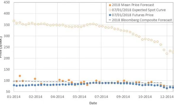
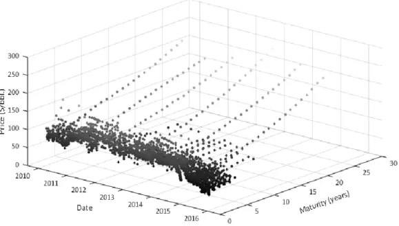
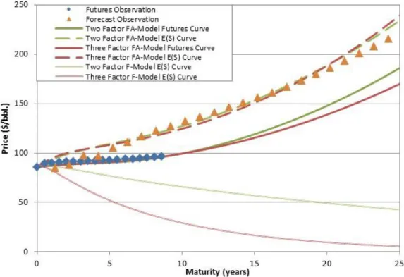
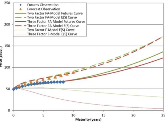
(6) LIST OF FIGURES Figure 1: Oil futures and expected spot curves under the two-factor model, oil futures prices and Bloomberg’s Median Composite for oil price forecasts, for 02-05-2014.......... 35 Figure 2: Analysts’ 2018 Oil Price Forecasts, Bloomberg Median Composite Forecast for 2018, Oil futures prices of contracts maturing close to 07-01-2018, and a Two-Factor Model expected spot at a 07-01-2018 maturity ................................................................... 36 Figure 3: Oil analysts’ price forecasts from 2010 to 2015 provided by Bloomberg’s Commodity Price Forecasts, World Bank (WB), International Monetary Fund (IMF) and U.S. Energy Information Administration (EIA). ................................................................. 37 Figure 4: Oil futures prices from 2010 to 2015 provided by NYMEX .............................. 38 Figure 5: Futures, expected spot curves and observations for 04-14-2010 ........................ 39 Figure 6: Futures, expected spot curves and observations for 07-22-2015 ........................ 40 Figure 7: Expected spot curves under the two and three-factor FA-, F- and A-Models, and forecasts observations, for 04-14-2010 ............................................................................... 41 Figure 8: Expected spot curves under the two and three-factor FA-, F- and A-Models, and forecasts observations, for 07-22-2015 ............................................................................... 42 Figure 9: Futures under the two-factor FA-, and F-Models, Expected spot curve under the two-factor FA-Model, forecasts and futures observations, for 04-14-2010 ........................ 43 Figure 10: Futures under the two-factor FA-, and F-Models, Expected spot curve under the two-factor FA-Model, forecasts and futures observations, for 07-22-2015 .................. 44 Figure 11: Futures under the three-factor FA-, and F-Models, Expected spot curve under the three-factor FA-Model, forecasts and futures observations, for 04-14-2010 ................ 45 Figure 12: Futures under the three-factor FA-, and F-Models, Expected spot curve under the three-factor FA-Model, forecasts and futures observations, for 07-22-2015 ................ 46 Figure 13: Annual model risk premium term-structure for the two and three-factor FAand F-Models, and annual mean data risk premiums .......................................................... 47. vi.

(7) LIST OF TABLES Table 1: Mean absolute error for the longest futures observation (9 years approx.) when the futures curve is calibrated using maturities up to 9 years (100%), futures only up to 4.5 years (50%), and futures only up to 2.25 years (25%) ........................................................ 48 Table 2: Oil analysts’ price forecasts from 2010 to 2015 grouped by maturity bucket ..... 49 Table 3: Oil futures prices from 2010 to 2015 grouped by maturity bucket ...................... 50 Table 4: Mean Annual Data Risk Premium from 2010 to 2015 by maturity bucket. ......... 51 Table 5: Two-factor F-Model and FA-Model parameters, standard deviation (S.D.) and tTest estimated from oil futures prices and price forecasts .................................................. 52 Table 6: Three-factor F-Model and FA-Model parameters, standard deviation (S.D.) and tTest estimated from oil futures prices and price forecasts .................................................. 53 Table 7: Price forecasts Mean Absolute Errors for the two and three factor F- and FAModels for each time window, between 2010 and 2015 ..................................................... 54 Table 8: Price forecasts Mean Absolute Errors for the two and three factor F- and FAModels for each maturity bucket, between 2010 and 2015 ................................................. 55 Table 9: Futures Mean Absolute Errors for the two and three factor F- and FA-Models for each time window, between 2010 and 2015........................................................................ 56 Table 10: Futures Mean Absolute Errors for the two and three factor F- and FA-Models for each maturity bucket, between 2010 and 2015. ............................................................. 57 Table 11: Two and three-factor A-Model parameters, standard deviation (S.D.) and t-Test estimated from oil analysts’ price forecasts ........................................................................ 58 Table 12: Expected Spot Mean Absolute Errors for the two and three factor FA- and AModels for each time window, between 2010 and 2015 ..................................................... 59 Table 13: Expected Spot Mean Absolute Errors for the two and three factor FA- and AModels for each maturity bucket, between 2010 and 2015 ................................................. 60 Table 14: Expected Spot Mean Price and Annual Volatility of the two-Factor FA- and AModels, for each equal size maturity bucket between 2010 and 2015 ................................ 61 Table 15: Expected Spot Mean Price and Annual Volatility of the three-Factor FA- and AModels, for each equal size maturity bucket between 2010 and 2015 ................................ 62 vii.

(8) Table 16: Futures Mean Price and Annual Volatility of the two-factor FA- and F-Models, for each maturity bucket between 2010 and 2015 ............................................................... 63 Table 17: Futures Mean Price and Annual Volatility of the three-factor FA- and F-Models, for each maturity bucket between 2010 and 2015 ............................................................... 64. viii.

(9) ABSTRACT Even though commodity pricing models have been successful in fitting the term structure of futures prices and its dynamics, they do not generate accurate true distributions of spot prices. This paper develops a new approach to calibrate these models using not only observations of oil futures prices, but also analysts´ forecasts of oil spot prices. We conclude that to obtain reasonable expected spot curves, analysts´ forecasts should be used, either alone, or jointly with futures data. The use of both futures and forecasts, instead of using only forecasts, generates expected spot curves that do not differ considerably in the short/medium term, but long term estimations are significantly different. The inclusion of analysts´ forecasts, in addition to futures, instead of only futures prices, does not alter significantly the short/medium part of the futures curve, but does have a significant effect on long-term futures estimations.. Keywords: Derivatives, commodities, pricing models, price forecasts, futures prices, expected spot prices.. ix.

(10) RESUMEN A pesar de que los modelos de precios de commodities han sido exitosos en ajustar la estructura de precios futuros y su dinámica en el tiempo, ellos no generan distribuciones de precios spot precisas. Este paper desarrolla un nuevo enfoque para calibrar estos modelos no solo usando observaciones de precios de futuros de petróleo, sino que también pronósticos de precios spot de petróleo realizados por analistas. Se concluye que para obtener curvas razonables de precios spot esperados se deben usar pronósticos de precios de analistas, tanto solos o conjuntamente con datos de precios de futuros. El uso de ambos sets, futuros y pronósticos, en contraste con el uso pronósticos únicamente, genera curvas de spot esperado que no difieren considerablemente en el corto/mediano plazo, aunque sí existen variaciones significativas en el largo plazo. Por otra parte, la inclusión de pronósticos realizados por analistas, sumados a los datos de precios futuros (en vez del uso de futuros únicamente), no altera significativamente la curva de futuros en el corto/mediano plazo, pero sí existe un efecto significativo en la estimación de precios futuros de largo plazo.. Palabras claves: Derivados, commodities, modelos de precios, pronóstico de precios, precios de futuros, precio spot esperado.. x.

(11) 1 1. 1.1. ARTICLE BACKGROUND Introduction A futures contract is financial derivative that establishes an obligation to exchange a. certain amount of underlying good at a given price and moment in the future. These contracts are traded at a surplus, or risk premium, over the expected spot price of the underlying asset at the contract’s maturity, to compensate for the risk of price deviations until that moment. Commodity futures are mainly used to secure the price of a specific commodity, such as oil, at a certain time horizon.. Since the last decades, stochastic commodity pricing models have gained wide acceptance among practitioners due to their performance at estimating the term structure of futures and their dynamics over time. When calibrated using various stochastic risk factors and adequate estimation methodologies, such as the Kalman Filter, they are able to model the contracts’ price variations in an extensive range of commodity markets.. Most commodity pricing models rely only on derivatives prices (futures and/or options) to calibrate all parameters, including the risk premium parameters. As Cortazar et al. (2015) showed, these parameters are generally measured with large errors and are not statistically significant. Therefore, the underlying expected spot prices are estimated to be very unreliable, even though they are important, limiting the overall credibility of these pricing models. Expected spot prices are fundamental when analyzing risk management (i.e. when calculating Value at Risk), and for investment evaluations, when practitioners compute their present value by discounting the expected prices by the weighted average cost of capital. To overcome this estimation difficulty, they study the incorporation of external information (futures returns given by a Capital Asset Pricing Model) on commodity pricing models, and prove it can be helpful in estimating the risk premium parameters..

(12) 2 In a similar attempt, we propose the use of financial analyst price forecasts, which have been generally ignored by the literature. Financial analysts issue periodical mean price estimations for a certain future term (quarterly or yearly), and this information is contained in economic reports or financial software like Bloomberg. Typically, both sets of data (futures and forecasts’ prices) are not used together when calibrating the commodity pricing models’ parameters, and they do not allow the integration of expectations information into their data panels.. The main hypothesis in this investigation is that by generating a model that incorporates analyst’s price predictions it is possible to correct the expected spot curve estimated by commodity pricing models, as well as producing a long term futures curve that relates to these estimations.. The rest of this work is organized as follows: Section 1.2 exposes the main objectives of this paper, Section 1.3 presents a review of the literature related to the topic of interest, while Section 1.4 shows the main conclusions delivered in this investigation. In addition, Section 1.5 proposes further research to be done that will improve the understanding of the use of both data sets, futures and forecasts, in commodity pricing models. Chapter 2 includes the article of this thesis. Section 2.1 introduces the subject and purpose of the paper, while section 2.2 shows the main challenges to be solved. Section 2.3 presents the commodity pricing model proposed and its calibration method, whereas Section 2.4 describes the data used to obtain the main results, shown in Section 2.5. Section 2.6 concludes the article.. 1.2. Main Objectives As explained previously, the information contained in both data sets (futures and. forecasts) can complement each other to improve the estimation of the term structure of futures and expected spot prices at any point in time. In this way, the first objective is to formulate a novel joint-estimation model which incorporates futures prices and analyst.

(13) 3 predictions, and uses this information to provide sound estimates of both the futures curve and the expected spot curve. The nature of analysts’ published opinion over the price of oil in the future represents a challenged that must be addressed. Price forecasts are very volatile (changing over time) dispersed (analysts provide very different mean price estimates for the same period in the future). This fact enhances the importance of estimating a consensus curve that can optimally use the price forecasts’ information. A second objective we wish to focus on is estimating a continuous term-structure of the market’s expected spot prices. Simple composite forecasts, such as Bloomberg’s Median Price Forecast, are easy to implement but naïve, and fail to provide expected spot point estimations for every future maturity, especially when panels are not complete (this is, not having a price estimation for every maturity at every moment in time). The time-dependent number of observations is an important issue that can be effectively handled using the Kalman Filter. In the case of price forecast data, the missing information problem is even more evident than in commodity futures prices (Cortazar and Naranjo (2006)) or bond yields (Cortazar et al. (2007)), emphasizing the need of a parameter estimation method that can successfully deal with this issue.. Apart from providing unreasonable estimates for expected spot prices, pricing models calibrated solely with futures contracts extrapolate futures prices badly for terms where no contracts are traded. Commodity futures have relatively short maturities (i.e. maximum 9 years for oil), and there is a need of having credible long-term commodity futures price estimations in order to hedge large investments on long-lasting projects (i.e. natural resource projects may last over 50 years). A third goal of this work is to provide reasonable long-term price estimations, by incorporating the information contained in analysts’ predictions into the commodity pricing models. The complementary forecasts data can be helpful when estimating credible long-term futures prices, if the price expectations correspond to longer maturities than the contracts traded. In this way, the.

(14) 4 long-term futures curve would be consistent with the price forecasts information and their implied long-term risk premiums.. Finally, there is no empirical information about the term-structure of risk premiums the market expects for oil prices. The only attempt (to our knowledge) to calculate the empirical, implicit risk premiums from the comparison between forecast and futures prices is made by Bolinger et al (2006), who calculate the implicit risk premiums in EIA reports for natural gas (as the difference between the expected spot and future price for exactly the same maturity), and discover they are considerable. However, this simple analysis is made for 2000 to 2003, it is restricted to natural gas, and does not generate a model to construct the term-structure of risk premiums. A final objective we wish to target is to provide a sound term-structure of risk premiums that relates to the empirical data provided by financial analysts in their predictions. 1.3. Literature Review This is not the first attempt to study the information content of analysts’ predictions. of different economic variables present in financial markets. O’Brien (1987) studies forecasts of earnings per share as predictors for expected earnings in the U.S. stock market. The author finds that the predictive power of earnings forecasts highly depends on their date of publication; more recent estimations have better forecasting performance. O’Brien (1990) extends this work and intends to measure the predictive power of individual analysts comparing their estimations with realized earnings, in nine industries. Hail and Leuz (2006) use stock earnings forecasts to calculate the implied cost of capital of companies (as a weighted average according to the analysts’ precision), and apply an econometric model to explain its movements over time with legal-related economic variables. Koijen et al (2015) study returns forecasts of three different asset classes (global equity, currencies and fixed income), and find that these survey expectations predict returns negatively in both the cross section and time series. Zhang (2006) uses stock target price forecasts’ dispersion (computed as the standard deviation of forecasts) to measure the uncertainty present in the market towards the information that a company will release in.

(15) 5 the future. Bonini et al. (2010) and Bradshaw et al (2012) study the predictive content of target price forecasts in the stock market, under different measures of accuracy. Greenwood and Shleifer (2014) study different sources of stock returns expectations and discover they are highly inter-correlated, and positively correlated with the market’s history and level, suggesting they are mainly extrapolative estimations. Apart from the stock market, the analysis of analysts’ expectations is extended to other areas of interest. Pesaran and Weale (2006) use survey information on short-term forecasts of macroeconomic variables to develop a complete analysis on how respondents shape their expectations and how these can be modelled. They analyze whether survey expectations data can help enhance the forecasting performance of time-series econometric models, for inflation, consumer sentiment or consumer spending, among other variables. Bachetta et al. (2009) measure the predictability of returns in stock, foreign exchange, bond and money markets in different countries using survey expectations. Pedersen (2015) analyzes the effect of the Chilean Central Bank’s public inflation forecasts on private forecasters, finding that the main influence is present for the short-term predictions. Nevertheless, commodity price forecast information (like Bloomberg’s Commodity Price Forecast function) has been generally neglected by the financial literature; scarce analysis exists on this data source up to the moment, (Berber and Piana (2016), Atalla et. al (2016)), specially for long-term oil price predictions (Haugom et al. (2016)). Berber and Piana (2016) state that the Bloomberg data set is useful because price forecasts are a direct approximation to the market’s expectations, they represent point estimations to concrete and different horizons, and they are emitted by individual analysts that are experts in each specific commodity market (a desirable characteristic, as Da and Schaumburg (2011) also indicate for equity target price forecasts).. They use these price forecasts to test their predictive power for realized returns in the crude oil and copper markets. Baumeister and Kilian (2015) also test the predictive power of short-term oil price forecasts from the EIA (U.S. Energy Information Administration, a source of economic expectations information widely used by practitioners and modelers, as.

(16) 6 the author indicates) by comparing them with a model that uses a combination of forecasts to estimate future spot prices. A similar study is made by Wong-Parodi et al. (2006), assessing if the short-term forecasts from EIA are good predictors of spot prices, in comparison to traded futures prices. Furthermore, Haugom et al. (2016) focuses on forecasting long-term oil prices, and uses the EIA forecasts as reference for their own estimations, provided by a model that builds on the fundamental relationships between demand and supply.. Auffhammer (2007) uses the short-term forecasts from EIA of a number of variables (including oil price forecasts) to show that they are issued using an asymmetrical loss function. The author indicates EIA is the most important source of energy price forecasts in the US market, and that this source is widely used by policymakers, industry and modelers. Moreover, Pierdzioch et al. (2013b) extends this analysis specifically to oil price forecasts published by the European Central Bank. Pierdzioch et al. (2010) find solid empirical evidence of anti-herding for oil price forecasts in the SPF. In other words, they find that the public consensus forecast has a strong influence on individual forecasters, who tend to differentiate their estimations from it. If the forecasters’ reputation or income depends on their relative forecasting accuracy, price differentiation incentives exist among them. The authors argue that anti-herding provides explanatory evidence for the crosssectional dispersion that price forecasts show. However, this analysis is made for shortterm forecasts (maximum forecasting horizon is 1 year). Pierdzioch et al. (2013a) extend this analysis by studying nine metals, also finding strong evidence of rational anti -herding in them. According to Laster et al (1999), the anti-herding behavior does not generate distorsions over the mean of forecasts, but only in the variance (or dispersion) among them.. Moreover, Bewley and Feibig (2002) found that there is more tendency to herd. when there is more volatility in the asset or variable being forecasted (or in other words, more difficulty to predict it).. Singleton (2014) finds positive correlation between the level of disagreement among forecasters (measured as the standard deviation of forecasts for certain horizon) and the level of WTI oil price. The author argues that information asymmetries and speculative.

(17) 7 activity make prices deviate from fundamental variables that explain them, generating booms/busts that are positively correlated with the dispersion of price forecasts at the 1year ahead horizon. In this line, and using the short-term European Central Bank surveys (maximum 1-year horizon), Atalla et al. (2016) find statistical evidence that supports the fact that analysts’ disagreement on oil price forecasts reflects realized oil price volatility.. 1.4. Main Conclusions The joint estimation model proposed in this work incorporates both data from futures. contracts and analysts price expectations. These data sets are used to generate reliable term-structure estimates both for futures and expected spot prices, which are now calculated using statistically significant parameters.. With this methodology, stochastic. commodity pricing models build credibility as they no longer generate expected spot prices that are inconsistent with the market’s expectations.. The model presented allows the practitioners to choose whether using both data panels indistinctively. This is useful when constructing an optimal consensus curve for the analysts’ price forecasts, using only expectations data. The consensus curve provides a credible, continuous term structure for the expected spot prices, which has a better fit to analysts’ price forecasts than the expected spot curve generated by the estimation that includes futures prices.. Under the joint estimation, we provide a long-term futures curve that is consistent with analysts’ price expectation information. The extrapolation of the futures curve is now generated using statistically significant risk premium parameters, fact that allows longterm futures prices to depend on the market’s spot price expectations for terms in which no futures contracts are traded..

(18) 8 Finally, we find a positive, decreasing term structure of risk premiums for oil. This cross-sectional behavior is validated by the empirical risk premiums calculated from price forecast information. Our results are statistically significant at the 99% level. A possible extension to this methodology is the exploration of the use of stochastic risk-factors to specifically model the risk premium structure in the time series. The model presented in this paper assumes risk premiums are constant, but this restriction can be relaxed to allow them to change over time (as Bianchi and Piana (2016) hypothesize) in relation to empirical risk premiums, consequently reducing the estimation errors..

(19) 9 2.. COMMODITY PRICE FORECASTS, FUTURES PRICES AND PRICING MODELS. 2.1. Introduction Over the last decades, commodity pricing models have been very successful in fitting. the term structure of futures prices and its dynamics. These models make a wide variety of assumptions about the number of underlying risk factors, and the drift and volatility of these factors [Gibson, R. & Schwartz, E.S. (1990); Schwartz, E.S. (1997); Schwartz, E.S. & Smith, J. (2000); Cortazar, G. & Schwartz, E.S. (2003); Cortazar, G. & Naranjo, L. (2006); Cassasus, J. & Collin-Dufresne, P. (2005); Cortazar, G., & Eterovic, F. (2010); Heston, S. L. (1993); Duffie, D., J. Pan, & K. Singleton (2000); Trolle, A. B. & Schwartz, E. S. (2009); Chiang, I., Ethan, H., Hughen, W. K., & Sagi, J. S. (2015)].. The performance of commodity pricing models is commonly assessed by how well these models fit derivative prices. It is well known that derivative prices are obtained from the risk neutral or risk adjusted probability distribution (e.g. futures prices are the expected spot prices under the risk neutral probability distribution). These models also provide the true or physical distribution of spot prices, but this has not been stressed in the literature because they have mainly been used to price derivatives.. However, as Cortazar,. Kovacevic & Schwartz, (2015) point out, the latter is also valuable and is used by practitioners for risk management, NPV valuations, and other purposes.. Despite the diversity of commodity pricing models found in the literature, they all share the characteristic of relying only on market prices (e.g. futures and options) to calibrate all parameters. In these models the risk premium parameters are measured with large errors and typically are not statistically significant, making estimations of expected prices (which differ from futures prices on the risk premiums) inaccurate.. To solve this problem Cortazar et al. (2015) propose using an Asset Pricing Model (e.g. CAPM) to estimate the expected returns on futures contracts from which the risk.

(20) 10 premium parameters can be obtained, which results in more accurate expected prices. However, these prices depend on the particular Asset Pricing Model chosen.. This paper develops an alternative way to estimate risk-adjusted and true distributions that does not rely on any particular asset pricing model. The idea is to use forecasts of future spot prices provided by analysts and institutions who periodically forecast these prices, such as those available from Bloomberg and other sources. Thus, by calibrating the commodity pricing model with both futures prices and analysts’ forecasts, two different data sets are jointly used to calibrate the model. Analysts’ forecasts have been previously used in finance, but mostly for corporate earnings. For example, O’Brien (1987) studies forecasts of earnings per share as predictors of earnings in the U.S. stock market. O’Brien (1990) measures the predictive power of individual analysts comparing their estimations with realized earnings in nine industries. Hail and Leuz (2006) use stock earnings forecasts to calculate the implied cost of capital of companies. Zhang (2006) uses stock target price forecasts dispersion to measure information uncertainty. Bonini et al. (2010) and Bradshaw et al. (2012) study the predictive content of target price forecasts in the stock market, under different measures of accuracy. Analysts’ forecasts have also been used in other areas and markets. For example, Pesaran and Weale (2006) use survey information on short-term forecasts of macroeconomic variables to develop an analysis on how respondents shape their expectations on inflation, consumer sentiment or consumer spending. Bachetta et al. (2009) measure the predictability of returns in stock, foreign exchange, bond and money markets in different countries using surveys. The use of analysts’ forecasts in commodity markets, which is of interest in this paper, has been scarce and, in general, neglected. However, Bloomberg’s Commodity Price Forecasts have been subject to some analysis [Atalla et al. (2016), Haugom et al. (2016)]. Berber and Piana (2016) state that this data set is useful because price forecasts.

(21) 11 are a direct approximation to the market’s expectations since they are made by individual analysts that are experts in each specific commodity market. They use these price forecasts to test their predictive power for realized returns in the crude oil and copper markets.. Another valuable source of commodity forecasts is the EIA (U.S. Energy Information Administration). Baumeister and Kilian (2015) use these data to test the predictive power of short-term oil price forecasts by comparing them with a model that uses a combination of forecasts to estimate future spot prices. A similar study is made by Wong-Parodi et al. (2006), assessing if the short-term forecasts from EIA are good predictors of spot prices, in comparison to traded futures prices. Furthermore, Haugom et al. (2016) focus on forecasting long-term oil prices, and use the EIA forecasts as a reference for their own estimations provided by a model that is built on the fundamental relationships between demand and supply. Auffhammer (2007) analyzes the rationality of EIA short-term forecasts. Bolinger et al. (2006), using only EIA reports from 2000 to 2003 natural gas contracts, estimate empirical risk premiums.. Other analysis on forecasting of commodity prices include Pierdzioch et al. (2010) and (2013b) on oil price forecasts published by the European Central Bank, Pierdzioch et al. (2013a) extending the anti-herding evidence to nine metals, Singleton (2014) on the disagreement among forecasters and the level of WTI oil price, and Atalla et al. (2016) on the fact that analysts’ disagreement on oil price forecasts reflects realized oil price volatility. In this paper, by proposing to use both market data (futures prices) and analysts’ forecasts (expected prices) to calibrate a commodity pricing model, several related objectives are pursued.. The first one is to formulate a joint-estimation model that. considers both sets of data and show how to estimate it using the Kalman Filter. Acknowledging that analysts’ price forecasts are very volatile, both because at any point in time there is great disagreement between them, and also because their opinions.

(22) 12 change greatly over time, our second objective is to build an analysts’ consensus curve that optimally aggregates and updates all their opinions.. Our third objective is to improve estimations for long-term futures prices. This is motivated by current practice which consists in calibrating commodity pricing models using futures with maturities only up to a few years and then is silent about whether the model will behave well for longer maturities. However, there is evidence that extrapolating a model calibrated only with short/medium term prices to estimate long term ones is unreliable [Cortazar, G, Milla, C. & Severino, F. (2008)]. In this paper, long term futures price estimations will be obtained by using also information from analysts’ forecasts.. Finally, the fourth objective is to estimate the term structure of the commodity risk premiums. This can be done by comparing the term structure of expected spot and futures prices.. The paper is organized as follows. To motivate the proposed approach, Section 2 provides empirical illustrations of some of the weaknesses of current approaches. Section 3 describes the model and parameter estimation technique used, while Section 4 describes the data set. The main results of the paper are presented in Section 5. Section 6 concludes.. 2.2. The Issues In what follows some of the issues that will be addressed in this paper are described.. The first issue, already pointed out in Cortazar et al. (2015), is that expected prices under the true distribution are unreliable when calibrating a commodity pricing model using only futures contract prices. As an illustration, Figure 1 shows the futures and expected oil prices for 02-05-2014 using the Cortazar and Naranjo (2006) two-factor model 1. It can be seen that while the 4.5 year maturity futures price is 77.9 US$/bbl., the model’s expected price, for the same maturity, is 365.8 US$/bbl. To justify that this expected price is 1. As shown in Cortazar and Naranjo (2006) this two-factor specification is equivalent to the Schwartz and Smith (2000) model, but may easily be extended to N-factors..

(23) 13 unreasonable, the Bloomberg’s Analysts´ Median Composite Forecast for 2018, which amounts to only 96.5 US$/bbl., is also plotted. Figure 2 shows the model expected spot prices, futures prices and analysts’ forecasts for a contract maturing around 07-01-2018 during the year 2014. It can be seen that the model expected spot prices are for the whole year around three times higher than the futures prices and analysts’ forecasts. Given that we will make use of a diverse set of analysts’ forecasts, a second issue is how to optimally generate and update an analysts’ consensus curve, as new information arrives. Figure 2 illustrates how the mean price forecasts for 2018 changes every week as new analysts provide their forecasts during 2014. It also shows that these forecasts are close to the corresponding futures prices, but the expected prices from the two-factor commodity model, when estimated using only futures, are much higher. Some efforts to provide an analysts’ consensus curve have already been made (the Bloomberg Median Composite, also plotted in Figure 2, but in general they are computed using only simple moving averages of previous forecasts.. Another and related issue is how to obtain credible estimations of commodity risk premiums. When expected spot prices are unreliable, risk premiums are also unreliable.. The final issue that will be addressed is how to obtain long-term futures price estimations that exceed the longest maturity contract traded in the market, using the information contained in long term analysts´ forecasts. Cortazar et al. (2008) already showed that extrapolations are unreliable: even if commodity pricing models fit well existing data, contracts with longer maturities are estimated with large errors.. To illustrate the point discussed above, a two factor model is calibrated using three alternative data panels of oil futures: all futures including maturities up to 9 years (100%), futures only up to 4.5 years (50%), and futures only up to 2.25 years (25%). For each data.

(24) 14 panel pricing errors for the longest observed futures price are computed. Table 1 shows that the longer the extrapolation, the higher the errors 2.. 2.3. The Model. 2.3.1 The N-Factor Gaussian Model. The Cortazar and Naranjo (2006) nonstationary N-factor model is chosen to illustrate the benefits of using analysts’ forecasts, in addition to futures prices. This model nests several well-known commodity pricing models (e.g. Brennan and Schwartz (1985), Gibson and Schwartz (1990), Schwartz (1997), Schwartz and Smith (2000), Cortazar and Schwartz (2003)) and lends itself easily to be specified with any number of risk factors.. Following Cortazar and Naranjo (2006), the stochastic process of the (log) spot price ( ) of a commodity is: (1) where. is the (. ) vector of state variables and. is the log-term price growth. rate, assumed constant. The vector of state variables follows the stochastic process: (2) where. and. are (. first element of. ) diagonal matrices containing positive constants (with the , and. is a set of correlated Brownian motions such that. , with each element of. being. . The risk adjusted process. followed by the state variables is: (3) where. is a (. ) vector containing the risk premium parameters corresponding to. each risk factor, all assumed to be constants.. 2. Differences are significant at the 99% confidence level..

(25) 15 Under the N-Factor model, the futures price at time , of a contract maturing at , can be obtained by computing the conditional expected value of the spot price, under the riskadjusted measure: (4). As shown in Cortazar and Naranjo (2006), this boils down to: (5) where, (6). (7). Similarly, it can be shown that the expected spot price for time. at time , is defined. by: (8) where, (9). Note that the only differences between the futures and expected spot dynamics are the risk premium parameters. Also, if these parameters were zero, the futures and expected spot prices would be equal. Define: (10) where. is the futures’ risk premium, given by: (11).

(26) 16 Finally, the model implied volatility (assumed to be constant in the time-series) is given by: (12) In this paper analysts’ forecasts are assumed to be noisy proxies for expected future spot prices. 2.3.2 Parameter Estimation A Kalman filter that incorporates futures prices and analysts’ forecasts into the process of estimating all parameters is applied. The Kalman Filter has been successfully used with incomplete data panels in commodities (Cortazar and Naranjo (2006)) and bond yields (Cortazar et al. (2007)), among others. Let’s define. as the time-variable number. of observations available at time .. The application of the Kalman Filter requires two equations to be defined: a) The transition equation, which describes the true evolution of the state variables ( over each time step ( ):. vector of. (13) where. is a. matrix,. is a. disturbances with mean 0 and covariance matrix. vector and. is an. vector of. .. b) The measurement equation, which relates the state variables to the log of observed futures prices and analysts’ forecasts: (14) where. is a. vector,. is a. matrix,. is a. vector of disturbances with mean 0 and covariance matrix. vector and .. is a.

(27) 17 Analysts provide their price forecasts as an annual average, instead of a price for every maturity, as is the case for futures. Thus, Equations (5) and (8) become (15). (16). Notice that in order to measure the analysts’ forecast observations we numerically approximate the mean annual price as the mean of. observations evenly spaced over the. same year of the estimation. As can be observed, unlike futures prices, price forecasts are not a linear function of the state variables.. In order for expected spot prices to be normally distributed, under the N-Factor model, the. must be represented by a linear combination of the state variables. This. can be achieved by linearizing the measured. when computing each. measurement step of the Kalman Filter 3.. If. and. are defined as the number of observations of futures prices and. analysts’ forecasts at time , the matrices corresponding to the measurement equation are: (17) where. is a. vector containing the futures observations and. is a. vector containing the price forecasts observations. Let (18) and (19). 3. More information on this methodology can be found in Cortazar, Schwartz, Naranjo (2007)..

(28) 18 where. is a. matrix and. equations for the futures data and. is a is a. vector containing the measurement matrix and. is a. vector. containing the linearized measurement equations for the price forecasts data.. Finally, (20). where. and. are the diagonal covariance matrices. of measurement errors of futures and price forecasts observations.. 2.4. The Data. 2.4.1 Analysts’ Price Forecasts Data Analysts´ price forecasts are obtained from four sources: Bloomberg, World Bank (WB),. International. Monetary Fund. (IMF). and. the. U.S.. Energy Information. Administration (EIA).. The first source is the Bloomberg Commodity Price Forecasts. This data base provides information on the mean price of each following year, up to 5 years ahead, made by individual analysts from a wide range of private financial institutions. Even though the data has not been analyzed extensively in the literature, it has been recently recognized as a rich and unexplored source of information [Berber and Piana (2016), Bianchi and Piana (2016)].. The next three sources (WB, IMF, and EIA), provide periodic (monthly, quarterly or annually) reports with long-term, annual mean price estimations up to 28 years ahead. Most historical data is available since 2010. Among these three sources, the last one has received more attention in the literature. In particular, Berber and Piana (2016) and Bianchi and Piana (2016) use it for oil inventory forecasts, while Bolinger et al. (2006),.

(29) 19 Auffhammer (2007), Baumeister and Kilian (2015) and Haugom et al. (2016) focus on price forecasts. Finally, Auffhammer (2007) and Baumeister and Kilian (2015) claim this source is widely used by policymakers, industry and modelers. Figure 3 shows the analysts’ price forecasts from all four sources, between 2010 and 2015. It can be seen that short-term forecasts are more frequent, in contrast to long-term forecasts which are issued in a less recurring, but periodical, basis. Analysts’ price forecasts are made for the average of each year. Thus, for each forecast its maturity is computed as the difference (in years) between the issue date and the middle of the year of the estimation (01-July of each year). Price forecasts are grouped into weeks ending on the following Wednesday, and then averaged 4. Forecasts for the same year, which include past information, are discarded as in Bianchi and Piana (2016). Table 2 summarizes the data.. 2.4.2 Oil Futures Data Oil futures data is obtained from the New York Mercantile Exchange (NYMEX). Weekly futures (Wednesday closing), with maturities for every 6 months, are used. There are from 17 to 19 contracts per week. Futures data is much more frequent than analysts’ forecasts, as can be seen by comparing Figures 3 and 4. Table 3 summarizes the futures data by maturity buckets with similar number of observations. 2.4.3 Risk Premiums Implied from the Data As explained in Section 3.1, empirical risk premiums can be derived directly form the data by comparing analysts’ forecasts with futures prices of similar maturity5. Since oil futures contracts longest maturity does not exceed 9 years, it is not possible to calculate the. 4. This is similar to what Berber and Piana (2016) or Bianchi and Piana (2016) do when averaging forecasts corresponding to the same period of estimation. 5 Forecasts with more than one year of difference with the nearest future contract are not used to calculate data risk premiums..

(30) 20 data risk premiums exceeding this term. Then, if maturity. , and. is a price forecast at time , for. is its closest futures (in maturity) for the same date, following. Equation 10 the data risk premium corresponding to that time is computed as:. (21). The mean data risk premiums for each maturity bucket is presented in Table 4. Notice that the annual data risk premium is decreasing with maturity.. 2.5. Results This section presents the results from calibrating the Cortazar and Naranjo (2006) N-. factor model, described in Section 3, using different specifications and calibration data. Model specifications include two and three risk factors. In terms of the calibration data, two sets are available: futures prices (F) and analysts’ forecasts (A). Results using jointly both data sets (FA-Model), only-analysts’ data (A-Model), and the traditional only-futures data (F-Model), are presented. The behavior of the futures curve, the expected spot price curve and the risk premiums is analyzed.. 2.5.1 Joint Model Estimation (FA-Model) The Joint Model estimation, FA-Model, uses both the analysts’ price forecasts and futures data to calibrate the N-Factor Model for two and three factors. To motivate the discussion, Figures 5 and 6 illustrate the results for the futures and expected spot curves, under different specifications and calibrations, for two specific dates, one, on 04-14-2010, in the in sample period and the other, on 07-22-2015, in the out of sample period. Notice that in all cases the curves fit reasonably well the futures prices and analysts’ forecasts observations when using the FA-Model. On the contrary, when using the traditional FModel, the expected price curves are well below the analysts’ forecasts..

(31) 21 Tables 5 and 6 present the parameter values obtained using the Kalman filter and using weekly data from 2010 to 2014, for the two- and three-factor FA-Models, respectively6. It is worth noticing that by using this new FA approach most risk premium parameters λi are now statistically significant. As discussed previously, the F- and FA-Models estimate both the true and the riskadjusted distributions, from which futures prices and expected spot prices can be obtained. Futures price and analysts’ forecast errors for both models are computed and presented in Tables 7 to 10. Tables 7 and 8 show the mean absolute errors between analysts’ forecasts and model expected spot prices generated by the FA-Model versus the F-Model. It is clear that the FA-Model has a significantly better fit for all time windows and buckets, for both the two and the three factor models.. Furthermore, Tables 9 and 10 show the mean absolute errors between observed futures prices and model futures prices. As expected, the benefit of obtaining a better fit in the expected spot prices, by including analysts’ forecasts, comes at the expense of increasing the mean absolute error on the futures prices. Nevertheless, the error increase is only 1%.. In summary the FA-Model has the advantage of generating a more reliable expected spot curve, with only a moderate effect for the goodness of fit for the futures 7. The threefactor model performs moderately better than the two-factor model.. 6. Measurement errors for both data sets are assumed to be the same, estimating a single parameter. However, this assumption can be relaxed to allow different measurement errors for futures and forecasts, consequently affecting the parameter estimation process. Furthermore, different measurement errors can be used for different maturity buckets in each data set, as shown in Cortazar et al. (2015) or in Cortazar et al. (2007). 7 Moreover, the tradeoff between both effects can be modified by setting different specifications for the measurement error variances for futures and forecasts when implementing the Kalman Filter. As explained in Section 3, our results use a single ξ parameter for both futures and forecasts observations at all maturities..

(32) 22 2.5.2 Analyst Consensus Curve using only Analysts’ Forecasts (A-Model) In the previous section, futures and expected spot curves for the FA-Model, calibrated using both futures and analysts’ forecasts, were presented. In that setting each curve is affected by both sets of data. In this section we calibrate the model using only analysts’ forecasts, modeling only the dynamics of the spot price. Thus, the expected spot curve represents an analysts’ consensus curve that optimally considers all previous forecasts. Given that futures data is not used, no futures curve or risk premium parameters are obtained. Table 11 shows the A-Model parameters values for the two and three factor models. Given that the model is only required to fit analysts’ price forecasts, and not futures prices, the expected spot curve fits better in the A-Model than in the FA-Model, and much better than in the F-Model. For example, Figures 7 and 8 show the expected spot curves for both models and compares them with those of the F-Model, for two specific dates, one, on 04-14-2010, in the in sample period and the other, on 07-22-2015, in the out of sample period. Tables 12 and 13 compares the mean absolute errors of the analysts’ consensus curve in both models, for two and three factors, respectively. As expected, the A-Model that only uses analysts’ forecast data fits better this data than the FA-Model which includes also futures prices. This holds for every time window and maturity bucket.. Table 14 reports the expected spot mean price and annual volatility of the two-Factor FA- and A-Models, for each maturity bucket between 2010 and 2015.. The first two. columns of Table 14 show that for the two-factor model the mean expected spot prices for the FA- and A- models are similar, especially for short term maturity buckets 8. The last two columns report the volatility of expected prices obtained for the two models. Since the. However, this assumption can be relaxed to allow different measurement error variances according to the nature of each observation included in the parameter estimation process. 8. In fact, differences in mean prices are significant at the 99% level for maturity buckets over 10 years..

(33) 23 analysts´ forecasts are very noisy, the A-Model generates an analysts’ consensus curve which is between 3 and 7 times more volatile than the one from the FA-Model. Table 15 reports the results for the three-factor model, which are similar to the ones in the two-factor model. In summary, the analysts’ consensus curve can be obtained from the FA or the AModels. The former has the advantage of generating a less volatile curve, while the latter generates a better fit. The difference between the means of both curves increases with maturity.. 2.5.3 Long-Term Futures Price Estimation using also Analysts’ Price Forecasts (FA-Model) As has been argued earlier, estimation of long term futures prices done by extrapolation is subject to estimation errors. Also, oil futures’ longest maturity is around 9 years, while there are oil price forecasts for maturities of over 25 years. In this section, the impact on long-term futures prices of using analysts’ price forecasts, in addition to traded futures, is explored.. To motivate this section Figures 9 and 10 show futures curves from the two factor FA- and F-Models, for two specific dates, one, on 04-14-2010, in the in sample period and the other, on 07-22-2015, in the out of sample period, and compares them to the analysts’ forecasts for the same dates. It can be seen that both futures curves for long maturities are very different. On the other hand, both curves are very similar for short and medium term maturities, for which there is futures data. Figures 11 and 12 present a similar situation for the three-factor model. Given that there are no long term futures to validate any of the curves, we present the FA-Model futures curve as a valuable alternative to the traditional F-Model curve, which takes into consideration analysts’ opinions..

(34) 24 Table 16 and Table 17 show the mean price and annual volatility of the futures curves (FA- and F-Models) for every maturity, for the two and three factor models, respectively. As the tables show, the inclusion of expectations data, when using the FAModel, significantly affects the mean futures curve in the long-term, without considerably changing it in the short-term. Again, as was the case for the expected spot curves in the previous section, the longer the maturity the greater the difference between both curves 9. Given the fact that analysts’ forecasts are very volatile, the effect of using them almost doubles the volatility of the futures curves when using the FA-Model.. 2.5.4 Data Risk Premium Curves Having reliable expected spot and the futures curves allows for the estimation of the term structure of risk premiums implied by their difference.. As stated earlier the. calibration of the F-Model provides statistically insignificant risk premium parameters, thus expected spot curves are unreliable. On the contrary, adding analysts´ forecast data addresses this issue.. Figure 13 shows the model term structure of risk premiums implicit in the difference of the expected spot and futures curves for the two and three factor FA- and F- Models. In these models the risk premium depends only on maturity and not on the state variables, so there is a constant risk premium curve for each model over the whole sample period. The figure also shows the data risk premiums, obtained directly from the difference between price forecasts and their closest future price observation, averaged for each maturity over the whole sample period 2010 and 2015, along with the 99% confidence interval.. Several insights can be gained from Figure 13. First, the FA-model risk premiums are very close to the mean data risk premiums. Second the three-factor model fits better the risk premiums than the two factor model, especially for short term maturities. Third, the. 9. Differences in mean curves are significant at the 99% level for maturity buckets from 10 to 25 years, for the two and three factor models..

(35) 25 term structure seems to be downward sloping, with annual risk premiums in the range of 2 to 10%. Finally, as expected, the F-Model is not able to obtain a credible estimation of risk premiums.. 2.6. Conclusion Even though commodity pricing models have been successful in fitting futures. prices, they do not generate accurate true distributions of spot prices. This paper proposes to calibrate these models using not only observations of futures prices, but also analysts´ forecasts of spot prices.. The Cortazar and Naranjo (2006) N-factor model is implemented for two and three factors, and estimated using the Kalman Filter. Each implementation is calibrated using the traditional only-futures data (F-Model), an alternative only-analysts’ data (A-Model), and a joint calibration using both sets of data (FA-Model).. Futures data is from NYMEX. contracts, and analysts´ forecasts from Bloomberg, IMF, World Bank, and EIA. Weekly oil data from 2010 to 2015 is used.. There are several interesting conclusions that can be derived from the results presented. The first is that in order to obtain reasonable expected spot curves, analysts´ forecasts should be used, either alone (A-Model), or jointly with futures data (FA-Model). Second, using both futures and forecasts (FA-Model), instead of using only forecasts (AModel), generates expected spot curves that do not differ considerably in the short/medium term, but long term estimations are significantly different and the volatility of the curve is substantially reduced. Third, the inclusion of analysts´ forecasts, in addition to futures, in the FA-Model, instead of only futures prices (F-Model) does not alter significantly the short/medium part of the futures curve, but does have a significant effect on long-term futures estimations, and increases the volatility of the curve. Finally, that in order to obtain a statistically significant risk premium term structure, both data sets must be used jointly, preferably using a three factor model..

(36) 26 The information provided by experts in commodity markets, reflected in analysts’ and institutional forecasts, is a valuable source that should be taken into account in the estimation of commodity pricing models. This paper is a first attempt in this direction..

(37) 27 REFERENCES Atalla, T., Joutz, F., & Pierru, A. (2016). Does disagreement among oil price forecasters reflect volatility? Evidence from the ECB surveys. International Journal of Forecasting, 32(1), 1178-1192. Auffhammer. (2007). The rationality of EIA forecasts under symmetric and asymmetric loss. Resource and Energy Economics, 29(1), 102-121. Bacchetta, P., Mertens, E., & van Wincoop, E. (2009). Predictability in financial markets: what do survey expectations tell us? Journal of International Money and Finance, 29(1), 406-426. Baumeister, C., & Kilian, L. (2015). Forecasting the real price of oil in a changing world: a forecast combination approach. Forthcoming: Journal of Business and Economic Statistics, 33(3), 338-351. Berber, A., & Piana, J. (2016). Expectations, fundamentals and asset returns: evidence from commodity markets. Working Paper. Bewley, R., Feibig, D.G. (2002). On the herding instinct of interest rate forecasters. Empirical Economics, 27 (1), 403-425. Bianchi, D., & Piana, J. (2016). Expected spot prices and the dynamics of commodity risk premia. Working paper. Bolinger, M., Wiser, R., & Golvone, W. (2006). Accounting for fuel price risk when comparing renewable to gas-fired generation: the role of forward natural gas prices. Energy Policy, 34(1), 706-720. Bonini, S., Zanetti, L. B., & Salvi, A. (2010). Target price accuracy in equity research. Journal of Finance and Accounting, 37(9), 1177-1217. Bradshaw, M., Brown, L., & Huang, K. (2012). Do sell-side analysts exhibit differential target price forecasting ability? Review of Financial Studies, 18(4), 930-955. Brennan, M., & Schwartz, E. (1985). Evaluating natural resources investments. Journal of Business, 58(2), 135-157. Cassasus, J., Collin-Dufresne, P. (2005). Stochastic convenience yield implied from commodity futures and interest rates. Journal of Finance. 60(5), 2283-2331. Chiang, I., Ethan, H., Hughen, W. K., & Sagi, J. S. (2015). Estimating oil risk factors using information from equity and derivatives markets. The Journal of Finance, 70(2), 769-804..

(38) 28 Cortazar, G., & Naranjo, L. (2006). An N-factor gaussian model of oil futures. Journal of Futures Markets, 26(3), 243-268. Cortazar, G., & Schwartz, E. (2003). Implementing a stochastic model for oil futures prices. Energy Economics, 25(3), 215-238. Cortazar, G., Kovacevic, I., & Schwartz, E. (2015). Expected commodity returns and pricing models. Energy Economics, 60-71. Cortazar, G., & Eterovic, F. (2010). Can Oil Prices Help Estimate Commodity Futures Prices? The Cases of Copper and Silver. Resources Policy, 35(4) 283–291 Cortazar, G., Milla, C., & Severino, F. (2008). A multicommodity model of futures prices: using futures prices of one commodity to estimate the stochastic process of another. Journal of Futures Markets, 28(6), 537-560. Cortazar, G., Schwartz, E., & Naranjo, L. (2007). Term-structure estimation in markets with infrequent trading. International Journal of Financial Economics, 12(4), 353-369. Duffie, D., J. Pan & K. Singleton (2000). Transform analysis and asset pricing for affine jump-diffusions. Econometrica 68 (6), 1343–1376. Gibson, R., & Schwartz, E. (1990). Stochastic convenience yields and the pricing of oil contingent claims. Journal of Finance, 45(3), 959-976. Greenwood, R., & Shleifer, A. (2014). Expectations of returns and expected returns. Review of Financial Studies, 27 (3), 714-746 Hail, L., & Leuz, C. (2006). International differences in the cost of equity capital: Do legal institutions and securities regulation matter? Journal of Accounting Research, 44(3), 485531. Haugom, E., Mydland, O., & Pichler, A. (2016). Long term oil prices. Energy Economics, 58 (1), 84-94. Heston, S. L. (1993). A Closed-Form Solution for Options with Stochastic Volatility with Applications to Bond and Currency Options. Review of Financial Studies 6 (2), 327–343. Koijen, R., Schmeling, M., Vrugt, E. (2014). Survey expectations of returns and asset pricing puzzles. Working paper. Laster, D., Bennett, P., Geoum, I.S. (1999). Rational bias in macroeconomic forecasts. Quarterly Journal of Economics, 114 (1), 293-318. O'Brien, P. (1987). Analysts' forecasts as earnings expectations. Journal of Accounting and Economics, 10(1), 58-83..

(39) 29. O'Brien, P. (1990). Forecast accuracy of individual analysts in nine industries. Journal of Accounting and Research, 10(1), 286-304. Pedersen, M. (2015). What affects the predictions of private forecasters? The role of central bank forecasts in Chile. International Journal of Forecasting, 31(1), 1043-1055. Pesaran, M., & Weale, M. (2006). Survey Expectations. Handbook of Economic Forecasting, 1(1), 715-776. Pierdzioch, C., Rülke, J., & Stadtmann, G. (2010). New evidence of anti-herding of oil price forecasters. Energy Economics, 32(1), 1456-1459. Pierdzioch, C., Rülke, J., & Stadtmann, G. (2013a). Forecasting metal prices: do forecasters herd? Journal of Banking and Finance, 37(1), 150-158. Pierdzioch, C., Rülke, J., & Stadtmann, G. (2013b). Oil price forecasting under asymmetric loss. Applied Economics, 45(17), 2371-2379. Schwartz, E. (1997). The stochastic behavior of commodity prices: implications for valuation and hedging. Journal of Finance, 52(3), 927-973. Schwartz, E., & Smith, J. (2000). Short-term variation and long-term dynamics in commodity prices. Management Science, 46(7), 893-911. Singleton, K. (2014). Investor Flows and the 2008 Boom/Bust in oil prices. Management Science, 60(2), 300-318. Trolle, A. B. & Schwartz, E. S. (2009). Unspanned Stochastic Volatility and the Pricing of Commodity Derivatives. Review of Financial Studies, 22(11): 4423–4461 Wong-Parodi, G., Dale, L., & Lekov, A. (2006). Comparing price forecast accuracy of natural gas models and futures markets. Energy Policy, 34(1), 4115-4122. Zhang, F. (2006). Information uncertainty and stock returns. Journal of Finance, 34(1), 105-137..

(40) 30. APPENDICES.

(41) 31. APPENDIX A: MODEL FURTHER SPECIFICATION A.1 The N-Factor Gaussian Model Matrices on Equation (2) are defined by:. (A.1). (A.2). and. is a set of correlated Brownian motions such that. ,. (A.3). where each element of. is. .. A.2 Parameter Estimation In this section we explain the process by which the Kalman Filter calculates the optimal state variables for each time step . Before each step, predictions of the level of the state variables are computed. If. is the covariance matrix of the estimation errors, the. estimators of the state variables for time at time. are:.

(42) 32 (A.4). (A.5) This enables the estimation of the observable variables for time :. (A.6). By using the new information that becomes available (contained in. ), the prediction. error ( ) and its covariance matrix ( ) are calculated:. (A.7). (A.8). The optimal estimates of the state variables up to time. are therefore estimated:. (A.9). (A.10). The vector of optimal parameter estimates ( ) is obtained by maximizing the loglikelihood function of error innovations:. (A.11). As shown in Equations (18) and (19), if we define. and. as the number of. observations of futures and price forecasts (respectively) at the same time , and. ,. as the sets containing their maturities, the matrices corresponding to the measurement equation are:.

(43) 33. (A.12). (A.13). (A.14). (A.15). Finally, the transition equation is independent of the nature and number of the observations, and therefore the matrices that define it stay the same as in the N-Factor model proposed by Cortazar and Naranjo (2006):. (A.16). (A.17).

(44) 34. (A.18).

(45) 35. APPENDIX B: FIGURES AND TABLES. Figure 1: Oil futures and expected spot curves under the two-factor model, oil futures prices and Bloomberg’s Median Composite for oil price forecasts, for 02-05-2014. The model is calibrated using weekly futures prices (01/2014 to 12/2014)..

(46) 36. Figure 2: Analysts’ 2018 Oil Price Forecasts, Bloomberg Median Composite Forecast for 2018, Oil futures prices of contracts maturing close to 07-01-2018, and a Two-Factor Model expected spot at a 07-01-2018 maturity. The model is calibrated using weekly futures prices (01/2014 to 12/2014)..

(47) 37. Figure 3: Oil analysts’ price forecasts from 2010 to 2015 provided by Bloomberg’s Commodity Price Forecasts, World Bank (WB), International Monetary Fund (IMF) and U.S. Energy Information Administration (EIA)..

(48) 38. Figure 4: Oil futures prices from 2010 to 2015 provided by NYMEX.

(49) 39. Figure 5: Futures, expected spot curves and observations for 04-14-2010. Curves include two and three-factor, FA- and F- Models. Parameter estimation from 2010 to 2014..

(50) 40. Figure 6: Futures, expected spot curves and observations for 07-22-2015. Curves include two and three-factor, FA- and F- Models. Parameter estimation from 2010 to 2014..

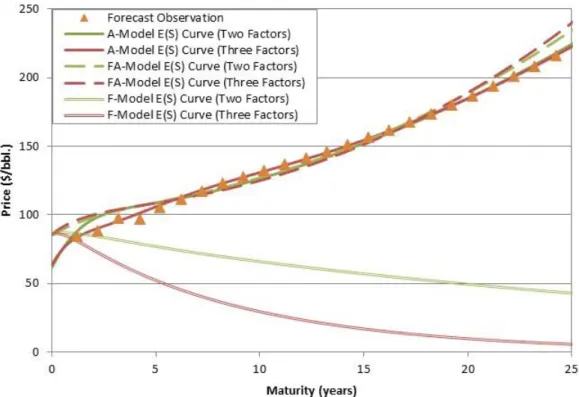
(51) 41. Figure 7: Expected spot curves under the two and three-factor FA-, F- and A-Models, and forecasts observations, for 04-14-2010. Parameter estimation from 2010 to 2014..

(52) 42. Figure 8: Expected spot curves under the two and three-factor FA-, F- and A-Models, and forecasts observations, for 07-22-2015. Parameter estimation from 2010 to 2014..

(53) 43. Figure 9: Futures under the two-factor FA-, and F-Models, Expected spot curve under the two-factor FA-Model, forecasts and futures observations, for 04-14-2010. Parameter estimation from 2010 to 2014..

(54) 44. Figure 10: Futures under the two-factor FA-, and F-Models, Expected spot curve under the two-factor FA-Model, forecasts and futures observations, for 07-22-2015. Parameter estimation from 2010 to 2014..

(55) 45. Figure 11: Futures under the three-factor FA-, and F-Models, Expected spot curve under the three-factor FA-Model, forecasts and futures observations, for 04-14-2010. Parameter estimation from 2010 to 2014..

(56) 46. Figure 12: Futures under the three-factor FA-, and F-Models, Expected spot curve under the three-factor FA-Model, forecasts and futures observations, for 07-22-2015. Parameter estimation from 2010 to 2014..

(57) 47. Figure 13: Annual model risk premium term-structure for the two and three-factor FA- and F-Models, and annual mean data risk premiums. The data risk premiums are implicit from the difference between price forecasts and their closest future price observation, for every date between 2010 and 2015, and are displayed along their 99% confidence intervals. Parameter estimation from 2010 to 2014..

(58) 48 Table 1: Mean absolute error for the longest futures observation (9 years approx.) when the futures curve is calibrated using maturities up to 9 years (100%), futures only up to 4.5 years (50%), and futures only up to 2.25 years (25%), from January 2010 to December 2015. The futures curve is obtained using the two factor model calibrated with oil futures weekly data from January 2010 to December 2014. (All differences between data panels are statistically significant al the 99% level). 100%. 50%. 25%. (Maturities from 0 to 9 yrs. Approx.). (Maturities from 0 to 4.5 yrs. Approx.). (Maturities from 0 to 2.25 yrs. Approx.). 0.9. 2.1. 18.5. Mean Absolute Error ($/bbl.).

(59) 49 Table 2: Oil analysts’ price forecasts from 2010 to 2015 grouped by maturity bucket. Forecasts are aggregated by week ending in the next Wednesday and averaged to obtain the mean price estimate for each following year in the same week. Maturity Bucket (years) 0-1 1-2 2-3 3-4 4-5 5-10 10-28 Total. Mean Price ($/bbl.) 88.4 93.9 96.8 95.5 93.0 99.1 165.9 100.9. Price S.D. 17.5 16.6 19.2 20.1 19.7 18.2 40.6 29.6. Mean Maturity (years) 0.8 1.5 2.5 3.5 4.5 6.7 16.9 4.1. Min. Price ($/bbl.) 47.2 52.3 50.9 51.5 52.0 61.2 80.0 47.2. Max. Price ($/bbl.) 117.5 135.0 189.0 154.0 140.0 153.0 265.2 265.2. N° of Observations 149 284 236 190 141 122 110 1232.

(60) 50 Table 3: Oil futures prices from 2010 to 2015 grouped by maturity bucket. Maturity Bucket (years) 0-1 1-2 2-3 3-4 4-5 5-6 6-7 7-8 8-9 Total. Mean Price ($/bbl.) 85.4 85.0 84.0 83.5 83.4 83.5 83.8 84.1 84.6 84.2. Price S.D. 17.7 14.5 12.7 11.6 11.0 10.8 10.9 11.1 11.6 12.8. Mean Maturity (years) 0.4 1.5 2.5 3.5 4.5 5.5 6.5 7.5 8.4 4.2. Min. Price ($/bbl.) 36.6 45.4 48.5 50.9 52.5 53.5 54.2 54.6 54.9 36.6. Max. Price ($/bbl.) 113.7 110.7 107.9 106.2 105.6 105.6 105.9 106.3 107.0 113.7. N° of Observations 786 621 625 627 631 622 625 626 461 5624.

(61) 51 Table 4: Mean Annual Data Risk Premium from 2010 to 2015 by maturity bucket. Maturity Buckets (years) 0.5 – 1.5 1.5 – 2.5 2.5 – 3.5 3.5 – 4.5 4.5 – 5.5 5.5 – 6.5 6.5 – 7.5 7.5 – 8.5 8.5 – 9.5. Mean Data Risk Premium (%) 7.6% 6.7% 5.2% 3.3% 2.9% 3.2% 3.2% 3.1% 3.0%.

(62) 52 Table 5: Two-factor F-Model and FA-Model parameters, standard deviation (S.D.) and tTest estimated from oil futures prices and price forecasts. Parameter estimation from 2010 to 2014. Parameter κ2 σ1 σ2 ρ12 μ λ1 λ2 ξ. F-Model Estimate S.D. t-Test 0.357 0.163 0.411 -0.407 -0.042 -0.041 0.004 0.010. 0.004 0.007 0.008 0.036 0.070 0.070 0.127 0.000. 90.638 23.617 50.204 -11.301 -0.600 -0.580 0.033 91.492. FA-Model Estimate S.D. t-Test 0.212 0.375 0.571 -0.885 -0.026 -0.003 0.068 0.046. 0.004 0.003 0.009 0.012 0.000 0.002 0.003 0.000. 53.522 149.492 64.496 -73.959 -55.725 -2.094 25.968 116.034.

(63) 53. Table 6: Three-factor F-Model and FA-Model parameters, standard deviation (S.D.) and tTest estimated from oil futures prices and price forecasts. Parameter estimation from 2010 to 2014. Parameter κ2 κ3 σ1 σ2 σ3 ρ12 ρ13 ρ23 μ λ1 λ2 λ3 ξ. F-Model Estimate S.D. t-Test 1.015 0.200 0.175 0.531 0.251 -0.162 -0.497 0.254 -0.123 -0.125 0.046 0.000 0.005. 0.011 0.003 0.003 0.006 0.004 0.003 0.007 0.004 0.068 0.068 0.189 0.001 0.000. 92.490 74.208 52.173 91.077 58.302 -59.458 -66.317 58.151 -1.818 -1.844 0.246 0.029 102.346. FA-Model Estimate S.D. t-Test 0.940 0.170 0.311 0.241 0.455 0.492 -0.809 -0.693 0.002 0.007 0.101 0.010 0.044. 0.023 0.004 0.003 0.004 0.008 0.010 0.015 0.012 0.000 0.003 0.009 0.007 0.000. 40.877 47.314 102.803 56.060 58.918 48.032 -52.635 -55.800 44.564 2.605 11.151 1.429 108.762.

(64) 54 Table 7: Price forecasts Mean Absolute Errors for the two and three factor F- and FAModels for each time window, between 2010 and 2015. Errors are calculated as percentage of price forecasts. Parameter estimation from 2010 to 2014.. Time Window In Sample (2010 – 2014) Out of Sample (2015) Total (2010 – 2015). N° of Observations 981 251 1232. Two Factors F-Model 24.7% 22.9% 24.3%. FA-Model 7.1% 6.3% 6.9%. Three Factors F-Model 38.6% 37.6% 38.4%. FA-Model 6.8% 6.0% 6.6%.

(65) 55 Table 8: Price forecasts Mean Absolute Errors for the two and three factor F- and FAModels for each maturity bucket, between 2010 and 2015. Errors are calculated as percentage of price forecasts. Parameter estimation from 2010 to 2014. Two Factors Buckets (years) 0-1 1-2 2-3 3-4 4-5 5-10 10-28 Total. N° of Observations 149 284 236 190 141 122 110 1232. F-Model 9.5% 14.7% 20.7% 23.5% 25.7% 35.5% 64.3% 24.3%. FA-Model 4.1% 5.3% 7.5% 9.2% 10.3% 7.1% 5.3% 6.9%. Three Factors F-Model 12.3% 22.1% 33.3% 40.7% 47.2% 61.1% 86.2% 38.4%. FA-Model 3.9% 4.9% 7.1% 8.9% 10.0% 6.9% 5.2% 6.6%.

(66) 56 Table 9: Futures Mean Absolute Errors for the two and three factor F- and FA-Models for each time window, between 2010 and 2015. Errors are calculated as percentage of futures prices. Parameter estimation from 2010 to 2014.. Time Window In Sample (2010 – 2014) Out of Sample (2015) Total (2010 – 2015). N° of Observations 4690 934 5624. Two Factors F-Model 0.7% 1.0% 0.8%. FA-Model 1.6% 2.6% 1.7%. Three Factors F-Model 0.3% 0.8% 0.4%. FA-Model 1.4% 1.8% 1.4%.

(67) 57 Table 10: Futures Mean Absolute Errors for the two and three factor F- and FA-Models for each maturity bucket, between 2010 and 2015. Errors are calculated as percentage of futures prices. Parameter estimation from 2010 to 2014.. Two Factors Buckets (years) 0-1 1-2 2-3 3-4 4-5 5-6 6-7 7-8 8-9 Total. N° of Observations 786 621 625 627 631 622 625 626 461 5624. F-Model 1.3% 0.9% 0.9% 0.7% 0.5% 0.4% 0.3% 0.6% 1.1% 0.8%. FA-Model 2.8% 1.7% 1.7% 1.5% 1.4% 1.4% 1.3% 1.5% 2.2% 1.7%. Three Factors F-Model 0.6% 0.5% 0.3% 0.4% 0.5% 0.4% 0.2% 0.3% 0.6% 0.4%. FA-Model 1.9% 1.7% 1.6% 1.5% 1.3% 1.2% 1.1% 1.1% 1.4% 1.4%.